
Evaluation of the Effectiveness of Anti-Turbulence Additives in the Transportation of High-Viscosity Oil at Low Ambient Temperatures


Abstract
1. Introduction
2. Theory of Calculation of the Hydraulic Resistance Coefficient When Using Anti-Turbulent Additives
3. Hydraulic Calculation Based on Additive Efficiency Data
Hydraulic Calculation Methodology
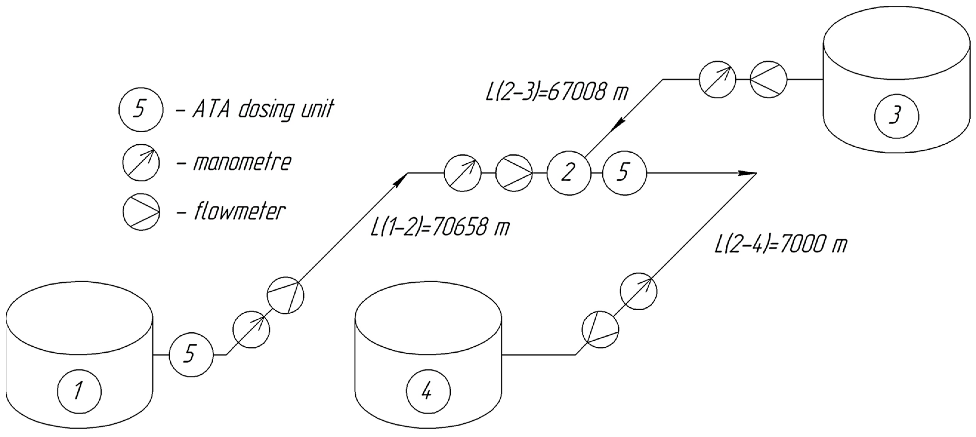
4. Pilot Testing of an Anti-Turbulence Additive
- Preparing the dosing equipment to ensure safe and uninterrupted operation during the trial.
- Injecting the anti-turbulence additive at a concentration of 40 g/t at the injection point.
- Filling the pipeline with oil and bringing the system to steady-state operation.
- Increasing the oil flow rate through the pipeline while maintaining steady-state conditions.
- Recording pressure and flow rate measurements over 24 h of pipeline operation under the dosing conditions of 40 g/t of additive.
- Reducing the flow rate to the initial values.
- Repeating steps 2-6 for additive concentrations of 50 g/t and 60 g/t.
- Stopping the injection of the additive into the pipeline.
- Processing the obtained results.
5. Results and Discussion
6. Conclusions
Author Contributions
Funding
Data Availability Statement
Conflicts of Interest
Abbreviations
| ATAs | Anti-turbulence additives |
References
- Shammazov, I.A.; Borisov, A.V.; Nikitina, V.S. Modeling the Operation of Gravity Sections of an Oil Pipeline. Bezop. Tr. v Promyshlennosti/Occup. Saf. Ind. 2024, 1, 74–80. (In Russian) [Google Scholar] [CrossRef]
- Pryakhin, E.I.; Azarov, V.A. Increasing the adhesion of fluoroplastic coatings to steel surfaces of pipes with a view to their use in gas transmission systems. Chernye Met. 2024, 3, 69–75. [Google Scholar] [CrossRef]
- Garashchenko, Z.M.; Teremetskaya, V.A.; Gabov, V.V. Mining of coal pillars using unified excavation modules with local faces. Russ. Min. Ind. 2024, 5S, 151–157. (In Russian) [Google Scholar] [CrossRef]
- Yifan, T.; Palaev, A.G.; Shammazov, I.A.; Yiqiang, R. Non-destructive testing technology for corrosion wall thickness reduction defects in pipelines based on electromagnetic ultrasound. Front. Earth Sci. 2024, 12, 1432043. [Google Scholar] [CrossRef]
- Litvinenko, V.S.; Dvoynikov, M.V.; Trushko, V.L. Elaboration of a conceptual solution for the development of the Arctic shelf from seasonally flooded coastal areas. Int. J. Min. Sci. Technol. 2021, 32, 113–119. [Google Scholar] [CrossRef]
- Bekibayev, T.; Zhapbasbayev, U.; Ramazanova, G.; Bossinov, D.; Pham, D.T. Oil pipeline hydraulic resistance coefficient identification. Cogent Eng. 2021, 8, 1950303. [Google Scholar] [CrossRef]
- Nikolaev, A.; Plotnikova, K. Study of the Rheological Properties and Flow Process of High-Viscosity Oil Using Depressant Additives. Energies 2023, 16, 6296. [Google Scholar] [CrossRef]
- Zakirova, G.; Pshenin, V.; Tashbulatov, R.; Rozanova, L. Modern Bitumen Oil Mixture Models in Ashalchinsky Field with Low-Viscosity Solvent at Various Temperatures and Solvent Concentrations. Energies 2023, 16, 395. [Google Scholar] [CrossRef]
- Burger, E.D.; Munk, W.R.; Wahl, H.A. Flow Increase in the Trans Alaska Pipeline Through Use of a Polymeric Drag-Reducing Additive. J. Pet. Technol. 1982, 34, 377–386. [Google Scholar] [CrossRef]
- Litvinenko, V.S.; Tsvetkov, P.S.; Dvoynikov, M.V.; Buslaev, G.V. Barriers to implementation of hydrogen initiatives in the context of global energy sustainable development. J. Min. Inst. 2020, 244, 428–438. [Google Scholar] [CrossRef]
- Fetisov, V.G.; Gonopolsky, A.M.; Zemenkova, M.Y.; Schipachev, A.M.; Davardoost, H.G.; Mohammadi, A.H.; Riazi, M.M. On the Integration of CO2 Capture Technologies for an Oil Refinery. Energies 2023, 16, 865. [Google Scholar] [CrossRef]
- Pshenin, V.V.; Zakirova, G.S. Increasing the efficiency of oil vapour recovery systems at commodity-transport operations at oil terminals. J. Min. Inst. 2024, 265, 121–128. [Google Scholar] [CrossRef]
- Dvoinikov, M.V.; Budovskaya, M.E. Development of hydrocarbon well completion system with low bottom-hole temperatures for conditions of oil and gas fields in Eastern Siberia. J. Min. Inst. 2022, 253, 12–22. [Google Scholar] [CrossRef]
- Korobov, G.Y.; Vorontsov, A.A.; Buslaev, G.V.; Nguyen, V.T. Analysis of Nucleation Time of Gas Hydrates in Presence of Paraffin During Mechanized Oil Production. Int. J. Eng. 2024, 37, 1343–1356. [Google Scholar] [CrossRef]
- Brostow, W. Drag reduction in flow: Review of applications, mechanism and prediction. J. Ind. Eng. Chem. 2008, 14, 409–416. [Google Scholar] [CrossRef]
- Nechval, A.M.; Muratova, V.I.; Chen, Y. Assessment of the influence of track degradation of an antiturbulent additive on its hydraulic efficiency. Transp. Storage Pet. Prod. Hydrocarb. Raw Mater. 2017, 1, 43–49. [Google Scholar]
- Coleman, B.P.; Ottenbreit, B.T.; Polimeni, P.I. Effects of a drag-reducing polyelectrolyte of microscopic linear dimension (Separan AP-273) on rat hemodynamics. Circ. Res. 1987, 61, 787–796. [Google Scholar] [CrossRef]
- Toms, B.A. Some Observations on the Flow of Linear Polymer Solutions Through Straight Tubes at Large Reynolds Numbers. Proc. First Int. Congr. Rheol. 1948, 2, 135–141. [Google Scholar]
- Malkin, A.Y.; Nesyn, G.V.; Manzhay, V.N.; Ilyushnikov, A.V. A new method of rheokinetic studies based on the use of the Toms effect. High Mol. Compd. Ser. B 2000, 42, 377–384. [Google Scholar]
- Chichkanov, S.V.; Shamsullin, A.I.; Myagchenkov, V.A. Influence of concentration of water-soluble polymer additives and turbulent flow velocity of straight oil emulsions on the magnitude of the Toms effect. Georesursy 2007, 3, 41–43. [Google Scholar]
- Korshak, A.A.; Hussein, M.N. Conditions for anti-turbulence additive effective use in the process of increasing oil pipeline capacity. Probl. Gather. Treat. Transp. Oil Oil Prod. 2008, 1, 42–44. [Google Scholar] [CrossRef]
- Abramov, I.P.; Dzardanov, O.I. Application of an antiturbulent additive in pumping diesel fuel through trunk pipelines of JSC ‘Ak Transnefteprodukt’. Notes Min. Inst. 2006, 167, 181–183. [Google Scholar]
- Pakhomov, M.A. Analysing the efficiency of methods to reduce hydraulic resistance of pipelines. Theory Pract. Mod. Sci. 2024, 8, 19–22. [Google Scholar]
- Konovalov, K.B.; Nesyn, G.V.; Manzhay, V.N.; Polyakova, N.M. Comparison of methods of production of antiturbulent oil additives based on laboratory data. Izv. Tomsk. Polytech. Universitet. Georesources Eng. 2011, 318, 131–135. [Google Scholar]
- Nesyn, G.V.; Suleymanova, Y.V.; Polyakova, N.M.; Filatov, G.P. Antiturbulent additive of suspension type on the basis of polymers of higher bb-olefins. Proc. Tomsk. Polytech. Univ. Georesources Eng. 2006, 309, 112–115. [Google Scholar]
- Ulyasheva, N.; Leusheva, E.; Galishin, R. Development of the drilling mud composition for directional wellbore drilling considering rheological parameters of the fluid. J. Min. Inst. 2020, 244, 454–461. [Google Scholar] [CrossRef]
- Konovalov, K.B.; Nesyn, G.V.; Polyakova, N.M.; Stankevich, V.S. Development of technology and assessment of production efficiency of antiturbulent additive of suspension type. Vectors Well-Being Econ. Socium 2011, 1, 104–111. [Google Scholar]
- Balabukha, A.V.; Inshakov, R.S.; Anisimova, E.Y.; Yasniuk, T.I.; Panasenko, N.L.; Vyazkova, E.A. Analytical methods for assessing the efficiency of application of anti-turbulence additives. Bull. Eurasian Sci. 2018, 10, 49. [Google Scholar]
- Virk, P.S. Drag reduction in rough pipes. J. Fluid Mech. 1971, 45, 225–246. [Google Scholar] [CrossRef]
- Virk, P.S. Drag reduction fundamentals. AIChE J. 1975, 21, 625–656. [Google Scholar] [CrossRef]
- Lurie, M.V.; Podoba, N.A. Modification of the Karman theory for the calculation of shear turbulence. Rep. USSR Acad. Sci. USSR 1984, 279, 570–575. (In Russian) [Google Scholar]
- Muratova, V.I. Evaluation of the Influence of Antiturbulent Additives on the Hydraulic Efficiency of Oil Product Pipelines. Ph.D. Thesis, Ufa State Petroleum Technical University, Ufa, Russia, 2014. [Google Scholar]
- Muratova, V.I.; Nechval, A.M. Choice of a formula for calculation of a hydraulic resistance coefficient at use of antiturbulent additives. Transp. Storage Oil Prod. 2008, 1, 11–13. (In Russian) [Google Scholar]
- Muratova, V.I.; Nechval, A.M. Determination of the effectiveness of anti-turbulent additives on the disc rheometer. In Proceedings of the Pipeline Transport—2013: The IX International Scientific and Practical Conference, Ufa, Russia, 18–20 March 2013; UGNTU Publishing House: Kigali, Rwanda, 2013; pp. 107–108. [Google Scholar]
- Chernikin, A.V. Generalised formula for the hydraulic resistance coefficient of pipelines. Transp. Storage Oil Prod. M. CNIITEneftekhim. 1997, 4–5, 20–22. [Google Scholar]
- Chernikin, V.A. Generalisation of calculation of the hydraulic resistance coefficient of pipelines. Hydrocarb. Sci. Technol. 1998, 1, 21–23. [Google Scholar]
- Chernikin, V.A.; Chernikin, A.V. Generalised formula for calculating the hydraulic resistance coefficient of main pipelines for light oil products and low-viscosity oils. Sci. Technol. Pipeline Transp. Oil Oil Prod. 2012, 8, 64–66. [Google Scholar]
- Chernikin, V.A.; Chelintsev, N.S. On improving the methods of determining the effectiveness of anti-turbulent additives on the main oil product pipelines. Sci. Technol. Pipeline Transp. Oil Pet. Prod. 2011, 1, 58–61. [Google Scholar]
- Karami, H.R.; Mowla, D. A general model for predicting drag reduction in crude oil pipelines. J. Pet. Sci. Eng. 2013, 111, 78–86. [Google Scholar] [CrossRef]
- Ozmen, Y.; Boersma, B.J. An experimental study on friction reducing polymers in turbulent pipe flow. Ocean. Eng. 2023, 274, 114039. [Google Scholar] [CrossRef]
- Nikolaev, A.F. The Toms Effect Using New Insights into the Structure of Water. J. Izv. St. Petersburg State Technol. Inst. 2009, 6, 76–79. [Google Scholar]
- MPMS 11.1-2004; Manual of Petroleum Measurement Standards Chapter 11—Physical Properties Data Section 1—Temperature and Pressure Volume Correction Factors for Generalized Crude Oils, Refined Products, and Lubricating Oils. American Petroleum Institute: Washington, DC, USA, 2004.
- Darcy, H. Les Fontaines Publiques de la Ville de Dijon: Exposition et Application des Principes à Suivre et des Formules à Employer Dans Les Questions de Distribution D’eau; V. Dalmont: Paris, France, 1857. [Google Scholar]
- Reynolds, O. An experimental investigation of the circumstances which determine whether the motion of water shall be direct or sinuous, and of the law of resistance in parallel channels. Philos. Trans. R. Soc. Lond. 1883, 174, 935–982. [Google Scholar] [CrossRef]
- Stokes, G.G. On the Effect of the Internal Friction of Fluids on the Motion of Pendulums. Trans. Camb. Philos. Soc. Part II 1851, 9, 8–106. [Google Scholar]
- Blasius, P.R.H. The law of similarity for friction processes in fluids. Mitteilungen über Forschungsarbeiten Auf Dem Geb. Ingenieurwesens 1913, 131, 1–41. [Google Scholar]
- Altshul, A.D. Hydraulic Resistance in Pipelines; Energiya Publishing: Moscow, Russia, 1948. [Google Scholar]
- Lumley, J.L. Drag Reduction by Additives. Annu. Rev. Fluid Mech. 1969, 1, 367–384. [Google Scholar] [CrossRef]
- Khalaf, A.N.; Abdullah, A.A. Simulation of crude oil transportation withdrag reduction agents using k-and k-x models. Eur. J. Comput. Mech 2021, 29, 459–490. [Google Scholar]
- Bogdevičius, M.; Janutėnienė, J.; Jonikas, K.; Guseinovienė, E.; Drakšas, M. Mathematical modeling of oil transportation by pipelines using anti-turbulent additives. J. Vi Broeng. 2013, 15, 419–427. [Google Scholar]
- Zhang, X.; Duan, X.; Muzychka, Y. New mechanism and correlation for degradation of drag-reducing agents in turbulent flow with measured data from a double-gap rheometer. Colloid Polym. Sci. 2018, 296, 829–834. [Google Scholar] [CrossRef]
- Den Toonder, J.M.J.; Draad, A.A.; Kuiken, G.D.C.; Nieuwstadt, F.T.M. Degradation effects of dilute polymer solutions on turbulent drag reduction in pipe flows. Appl. Sci. Res. 1995, 55, 63–82. [Google Scholar] [CrossRef]


| Pipe Section | Length, m | External Diameter, m | Internal Diameter, m | Volume, m3 |
|---|---|---|---|---|
| 1-2 | 70,658 | 0.325 | 0.309 | 5296 |
| 2-3 | 67,008 | 0.325 | 0.305 | 4893 |
| 2-4 | 7000 | 0.325 | 0.309 | 524 |
| № | Dosage of Additive, g/t | Flow Rate, t/h | Inlet Pressure, kgf/cm2 | Pressure Loss ΔP, kgf/cm2 | Theoretical Value of Drag Reduction, % | Hydraulic Resistance Coefficient |
|---|---|---|---|---|---|---|
| Pipe section 1-2 | ||||||
| 1 | Without ATA | 179.9 | 54.4 | 24.0 | - | 0.0340 |
| 2 | 40 | 289.8 | 57.8 | 26.2 | 36 | 0.0218 |
| 3 | 50 | 289.7 | 60.4 | 26.8 | 41 | 0.0201 |
| 4 | 60 | 289.8 | 63.0 | 27.1 | 45 | 0.0187 |
| Pipe section 2-4 | ||||||
| 1 | Without ATA | 179.9 | 54.4 | 24.0 | - | 0.0340 |
| 2 | 40 | 289.8 | 57.8 | 26.2 | 36 | 0.0218 |
| 3 | 50 | 289.7 | 60.4 | 26.8 | 41 | 0.0201 |
| 4 | 60 | 289.8 | 63.0 | 27.1 | 45 | 0.0187 |
| Name of Parameter | Value |
|---|---|
| Temperature at the beginning of the section, °C | 30 |
| Temperature at the end of the section, °C | 22 |
| Paraffin content, % | 2.62 |
| Density, kg/m3 | 873 |
| Kinematic viscosity (at 20 °C) | 36.7 mm2/s |
| Water content, % | 0.1 |
| Name of Parameter | Value |
|---|---|
| Appearance | White-colored suspension |
| Viscosity at 20 °C, mPa∙s | 167 |
| Viscosity at −40 °C, mPa∙s | 1015.8 |
| Density at 20 °C, kg/m3 | 876 |
| Solidification temperature, °C | Less than −50 |
| Particulate matter content, % | 37.8 |
| № | Dosage of Additive, g/t | Flow Rate, t/h | Inlet Pressure, kgf/cm2 | Outlet Pressure, kgf/cm2 | Pressure Loss ΔP, kgf/cm2 |
|---|---|---|---|---|---|
| 1 | Without ATA | 179.9 | 54.4 | 30.4 | 24.0 |
| 2 | 40 | 289.8 | 63.0 | 35.9 | 27.1 |
| 3 | 50 | 289.7 | 60.4 | 33.6 | 26.8 |
| 4 | 60 | 289.8 | 57.8 | 31.8 | 26.2 |
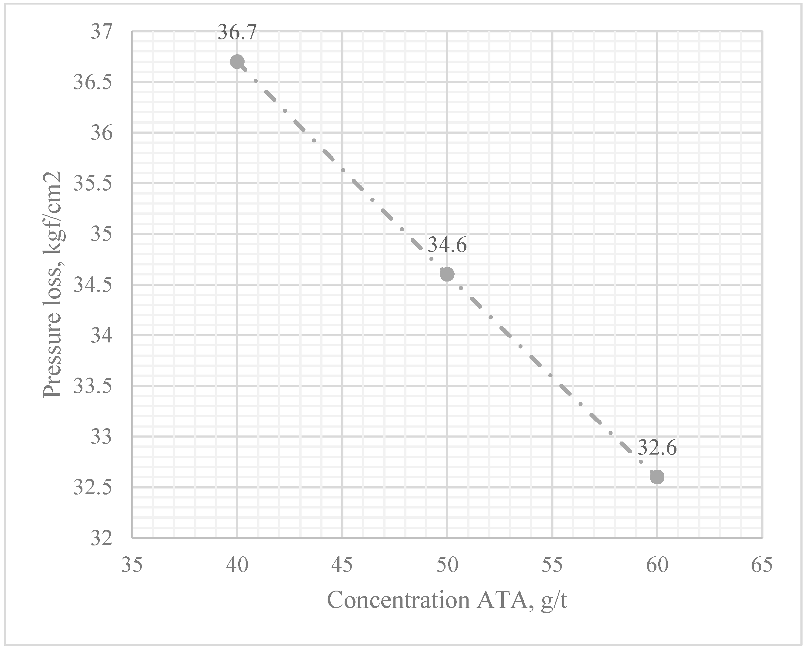
| № | Dosage of Additive, g/t | Flow Rate, t/h | Inlet Pressure, kgf/cm2 | Outlet Pressure, kgf/cm2 | Pressure Loss ΔP, kgf/cm2 |
|---|---|---|---|---|---|
| 1 | Without ATA | 198.4 | 37.8 | 4.4 | 33.4 |
| 2 | 40 | 305.4 | 39.5 | 2.8 | 36.7 |
| 3 | 50 | 307.5 | 41.4 | 6.8 | 34.6 |
| 4 | 60 | 307.4 | 43.8 | 11.2 | 32.6 |
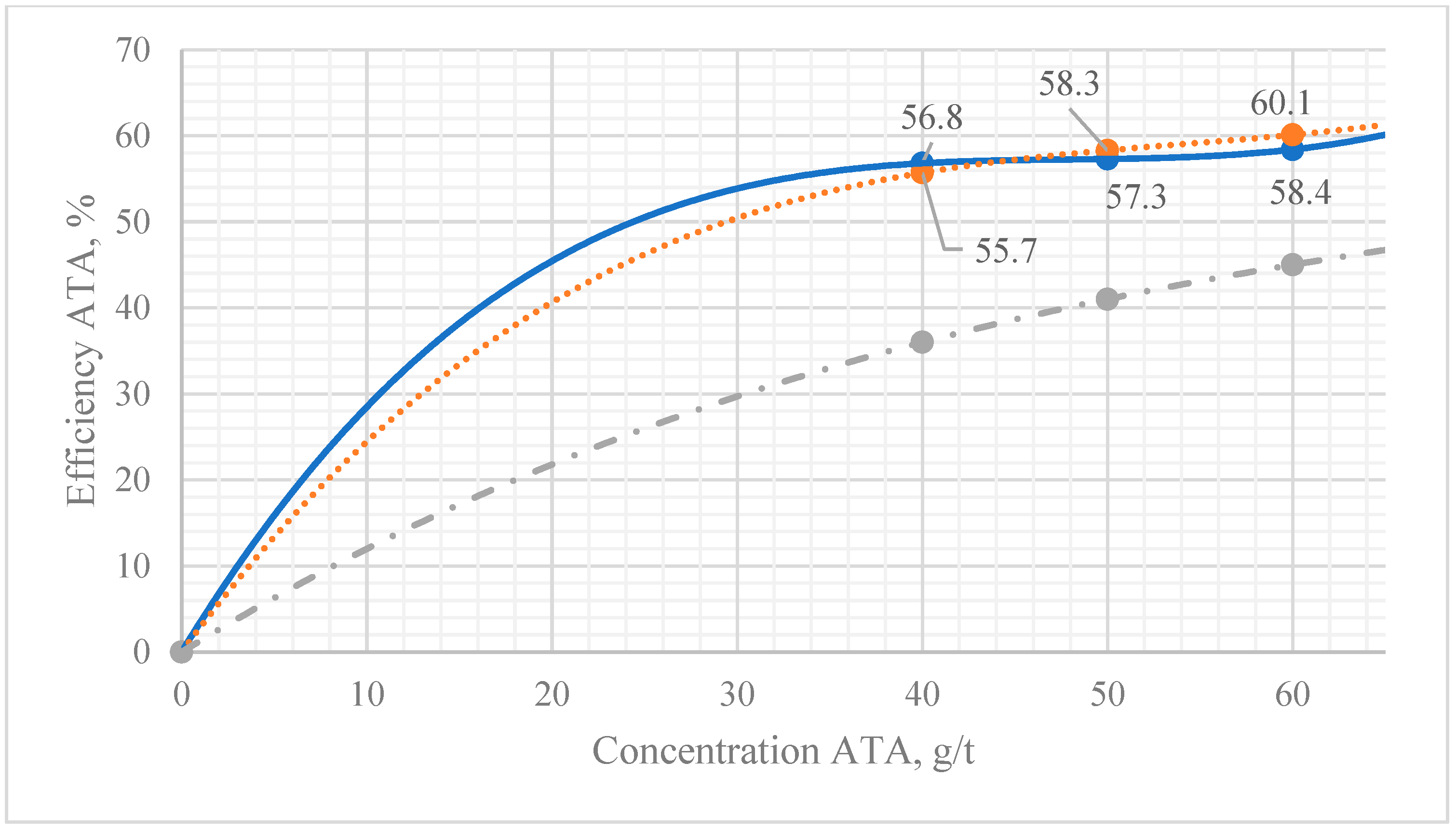
| № | Dosage of Additive, g/t | ATA Effectiveness, % (Section 1-2) | ATA Effectiveness, % (Section 2-4) | Calculated ATA Effectiveness, % |
|---|---|---|---|---|
| 1 | 40 | 55.7 | 56.8 | 36 |
| 2 | 50 | 57.3 | 58.3 | 41 |
| 3 | 60 | 58.4 | 60.1 | 45 |
| № | Dosage of Additive, g/t | Deviation of ATA Effectiveness, % (Section 1-2) | Deviation of ATA Effectiveness, % (Section 2-4) |
|---|---|---|---|
| 1 | 40 | 36.7 | 33.6 |
| 2 | 50 | 27.9 | 29.7 |
| 3 | 60 | 22.3 | 25.1 |
Disclaimer/Publisher’s Note: The statements, opinions and data contained in all publications are solely those of the individual author(s) and contributor(s) and not of MDPI and/or the editor(s). MDPI and/or the editor(s) disclaim responsibility for any injury to people or property resulting from any ideas, methods, instructions or products referred to in the content. |
© 2025 by the authors. Licensee MDPI, Basel, Switzerland. This article is an open access article distributed under the terms and conditions of the Creative Commons Attribution (CC BY) license (https://creativecommons.org/licenses/by/4.0/).
Share and Cite
Nikolaev, A.; Zhukov, A.; Goluntsov, A.; Shirmaher, E. Evaluation of the Effectiveness of Anti-Turbulence Additives in the Transportation of High-Viscosity Oil at Low Ambient Temperatures. Processes 2025, 13, 1434. https://doi.org/10.3390/pr13051434
Nikolaev A, Zhukov A, Goluntsov A, Shirmaher E. Evaluation of the Effectiveness of Anti-Turbulence Additives in the Transportation of High-Viscosity Oil at Low Ambient Temperatures. Processes. 2025; 13(5):1434. https://doi.org/10.3390/pr13051434
Chicago/Turabian StyleNikolaev, Alexander, Arkady Zhukov, Andrey Goluntsov, and Evgeniya Shirmaher. 2025. "Evaluation of the Effectiveness of Anti-Turbulence Additives in the Transportation of High-Viscosity Oil at Low Ambient Temperatures" Processes 13, no. 5: 1434. https://doi.org/10.3390/pr13051434
APA StyleNikolaev, A., Zhukov, A., Goluntsov, A., & Shirmaher, E. (2025). Evaluation of the Effectiveness of Anti-Turbulence Additives in the Transportation of High-Viscosity Oil at Low Ambient Temperatures. Processes, 13(5), 1434. https://doi.org/10.3390/pr13051434