Article

Development of a Computer-Aided Process for Recovering and Purifying 2-Methyl-2-Cyclopentenone Based on Measured Phase Equilibrium Data

1
Key Laboratory for Green Chemical Technology of Ministry of Education, R&D Center for Petrochemical Technology, Tianjin University, Tianjin 300072, China
2
Zhejiang Institute of Tianjin University, Ningbo 315201, China
3
State Key Laboratory of Engines, Tianjin University, Tianjin 300072, China
4
Tianjin Jiuyuan Chemical Engineering Co. Ltd., Tianjin 300072, China
*
Author to whom correspondence should be addressed.
Processes 2025, 13(5), 1435; https://doi.org/10.3390/pr13051435
Submission received: 12 February 2025 / Revised: 19 March 2025 / Accepted: 8 April 2025 / Published: 8 May 2025
(This article belongs to the Section Chemical Processes and Systems)

Abstract

:
2-Methyl-2-cyclopentenone (MCP) is the main by-product of the newly developed heterogeneous catalysis process for producing crotonaldehyde, which serves as an important intermediate for drug synthesis. However, how to recover and purify MCP from the product mixture is not known. To decipher this, a computer-aided process based on the measured phase-equilibrium data was developed. The improved Rose–Williams equilibrium kettle was used to measure the vapor–liquid equilibrium data for MCP–crotonaldehyde and MCP–water. Surprisingly, MCP and water formed a minimum azeotrope, which aided its own recovery from its dilute solution. The mole fraction of MCP in the azeotrope was 9.1%, the mole fraction of water was 90.9%, and the azeotropic temperature was 96.8 °C. Equilibrium data from the two binary systems were correlated using the Wilson and NRTL activity coefficient models. The NRTL-RK model was selected to simulate the process for recovering and purifying MCP. A two-column process was developed and optimized in this study, and the aim of effectively utilizing the by-product MCP was achieved with this process.

1. Introduction

Crotonaldehyde is an important raw material of fine chemicals. It can be used to prepare sorbic acid (2,4-Hexadienoic acid) [1], crotonic acid [2], and other C4 and C8 derivatives. Among them, the preparation of sorbic acid has gradually become the most important use of crotonaldehyde, because sorbic acid is a safe food preservative [3]. With the increasing demand for sorbic acid in the market, it is necessary to scale up the production of crotonaldehyde in the industry. The current production process of crotonaldehyde uses sodium hydroxide solution and acetic acid in a series for catalysis, which causes serious problems such as saline waste water and equipment corrosion [4].
Therefore, the chemical process of heterogeneous catalysis was explored, and Zr-β molecular sieves showed excellent performance in this process [5,6,7]. The application of Zr-β heteroatomic molecular sieve catalysts in the field of heterogeneous catalysis such as in acetaldehyde aldol condensation has been intensively studied by our group [8,9,10,11]. Yingying Zhao found that the main by-product of the preparation of acetaldehyde condensates using Zr-β molecular sieves as catalysts was 2-methyl-2-cyclopentenone (MCP). MCP is an important intermediate in drug synthesis. It can be used to synthesize various drugs such as vitamin B6.
MCP–crotonaldehyde vapor–liquid equilibrium data are required for the industrial production of crotonaldehyde from Zr-β heteroatomic molecular sieve-catalyzed acetaldehyde aldol condensation. MCP–water vapor–liquid equilibrium data are very important for the design of MCP and water separation processes.
However, there are no vapor–liquid equilibrium data in the literature for MCP and water and MCP and crotonaldehyde in a condensation reaction system. Experimental measurements are needed to solve this problem. Rose kettles are commonly used to measure vapor–liquid phase-equilibrium data, for example, the determination and correlation study of vapor–liquid equilibrium of hexanoic acid + acetic acid/butyl acetate/cyclohexanone/ε-caprolactone system at 20 kPa using a Rose equilibrium kettle by Yachun Chen [12]; the phase-equilibrium study of aromatic extraction system using N-formylmorpholine as a solvent using a Rose equilibrium kettle by Shuqian Xia [13]; and the collection of vapor–liquid equilibrium data of a methanol–formaldehyde–PODEn ternary system using a modified vapor–liquid equilibrium two-cycle Rose kettle by Pan Li [14]. The method for determining vapor–liquid phase-equilibrium data using a Rose equilibrium kettle is very reliable. Therefore, this study intends to use the improved Rose–Williams equilibrium kettle of Tianjin University for the determination of vapor–liquid equilibrium data. After the vapor–liquid equilibrium data were measured, a thermodynamic consistency check [15,16,17] was performed using the Gibbs–Duhem equation to determine whether the experimentally measured vapor–liquid equilibrium data were reliable for each group.
The experimental methods for determining the vapor–liquid equilibrium data of a system can generally be divided into direct methods and indirect methods. Direct methods mainly include the static method [18], flow method [19], and circulation method [20]. The static method has advantages such as easy equipment fabrication, high-pressure resistance, and good sealing performance. However, the equilibrium vessel used in experiments is bulky, consumes large amounts of the various reagents, and requires a long equilibration time. Additionally, during actual sampling and analysis, the original equilibrium state inside the vessel may be disrupted, leading to experimental errors. The flow method establishes vapor–liquid equilibrium dynamically, which can prevent issues like the polymerization or thermal decomposition of substances. However, its main drawbacks are the excessive sample quantity required and the difficulty in precisely controlling the flow rates of materials in the delivery system. The vapor–liquid dual-circulation method partially addresses the limitations of single-phase (vapor) circulation, reduces pressure requirements for the system, and is suitable for measuring the vapor–liquid equilibrium data under low or atmospheric pressure. Furthermore, this method offers advantages such as minimal material consumption, no dead zones in the circulation loop, and significantly reduced overheating and liquid entrainment during heating compared to single-phase circulation. Although direct methods are simple, easy to operate, and provide accurate data, they are not universally applicable. For systems containing low-boiling-point components, flash evaporation under high-pressure conditions may occur, leading to inaccuracies in data measurement. Indirect methods do not directly obtain composition data through experiments. Instead, they use measured saturated vapor pressures or boiling points of solutions with different compositions and solve the Gibbs–Duhem equation algorithmically to derive the vapor–liquid phase compositions.
Distillation is a separation technology that achieves multiple gas–liquid mass transfers by means of a tower plate or packing, which is suitable for mixtures with small differences in boiling points, and has the advantages of high efficiency and industrial maturity; it is widely used in petroleum fractional distillation and alcohol purification. However, it consumes high energy and is unable to separate the azeotropic system (e.g., ethanol–water) directly. In contrast, azeotropic distillation [21] successfully solves the problem of ethanol dehydration by introducing entraining agents (such as benzene or cyclohexane) to break the azeotrope; however, additional separation of the entraining agent is required, which makes the process complicated and may introduce contamination, but it is suitable for the special separation needs of azeotropic systems. Vacuum distillation [22] can avoid thermal decomposition caused by high temperatures by reducing the pressure of the system which makes the boiling point of the components drop significantly. It is especially suitable for the purification of high-boiling substances (such as heavy oils) or heat-sensitive substances (such as vitamins); however, its reliance on high-vacuum equipment leads to increased costs, and its mass transfer efficiency is limited. Overall, distillation is the first choice for conventional separation, azeotropic distillation is used when dealing with azeotropic systems, and vacuum distillation is used for high-boiling-point or heat-sensitive systems; the practical applications of these methods along with the characteristics of the mixture, the cost, and the purity requirements are assessed together to make an appropriate choice.
In this study, the vapor–liquid equilibrium data for MCP–crotonaldehyde and MCP–water were measured using the vapor–liquid two-cycle method using a Rose–Williams equilibrium kettle at 102 kPa. The experimental data were regressed using the Wilson and NRTL equations to derive the binary interaction parameters for each equation. The calculated values for all equations were in good agreement with the experimental values. Furthermore, based on the experimentally measured phase-equilibrium data, a separation process of MCP and water was designed and its parameters optimized.

2. Materials and Methods

2.1. Reagents and Apparatus

The experiment involves five chemical reagents, namely methanol, isopropanol, 2-methyl-2-cyclopenten-1-one (MCP), crotonaldehyde, and water. The specifications and manufacturers of these chemical reagents are listed in Table 1.
The instruments and equipment used in this experiment, as well as their manufacturers, are listed in Table 2.
This experiment uses the vapor–liquid equilibrium data measurement method with the improved Rose–Williams equilibrium kettle developed by Tianjin University. The material is heated and boiled in the boiling chamber, then sprayed into the equilibrium chamber in the form of a vapor–liquid mixture through an ascending pipe to establish vapor–liquid equilibrium. Under the action of gravity, the vapor and liquid phases are separated. The vapor phase is condensed and collected in the vapor phase tank through the condensation tube, while the liquid phase falls back into the liquid storage tank. As the liquid level in the storage tank gradually rises, the vapor phase flows back to the boiling chamber through the reflux tube, and the liquid phase overflows to the boiling chamber, forming a vapor–liquid double-cycle process. The main advantages of this apparatus are as follows: small sample size, fast equilibrium speed, and accurate vapor–liquid equilibrium data [23]. This apparatus is shown in Figure 1.

2.2. Experimentation

(1)
Fix the equilibrium kettle on the iron frame and add about 40 mL of a certain pure component of the binary system into the kettle. Connect the condensation tube and use high-vacuum grease to seal the joint. Add silicone oil into the temperature measurement sleeve, insert the precision thermometer, and turn on the cooling water.
(2)
Turn on the power supply. To avoid boiling over, preheat the apparatus at a lower voltage first. Then, slowly increase the voltage to around 125 V. When the liquid in the kettle begins to boil, observe the thermometer reading and the number of condensation droplets until the temperature stabilizes and the reflux droplet rate stabilizes at around 2 drops/s.
(3)
Record the temperature and reflux droplet rate every 15 min. When the reading remains stable for more than 1 h, it can be considered that the vapor–liquid equilibrium has been established. Record the equilibrium temperature, regulator voltage, and reflux droplet rate. The temperature difference during the constant temperature period is allowed to fluctuate within ±0.2 °C. Then, use a sampling needle to extract 0.1 mL of sample from the vapor and liquid sampling ports, respectively, and store them in 250 μL chromatographic bottles for measurement.
(4)
Use a 5 mL syringe to take out a certain amount of liquid from the kettle and add an equal amount of another component to change the composition of the material in the kettle. Repeat the above steps, by sampling and analyzing after a new equilibrium state is reached, and obtain the second, third, fourth, and further groups until the equilibrium temperature approaches the boiling point of the other component. To reduce measurement errors, each sampling point should be measured three times. The data can be used when the relative error between the three sets of data is less than 0.5%. The average of the three sets of data is taken as the final data.
(5)
After all data points have been sampled, turn off the regulator so that the apparatus starts to cool down. Wait for the condensation tube to have no liquid dripping and then turn off the cooling water and take out the liquid in the kettle. Clean the apparatus thoroughly.

2.3. Quantitative Analysis Method

In chromatographic analysis, because the same detector responds differently to different substances, the peak area (or height) produced when the same mass of different substances passes through the detector may not be the same. Therefore, in order to accurately reflect the content of the tested substance using peak area, a known amount of the test composition must be used to determine the correction factor so that the peak areas produced by the same concentration of different substances passing through the detector are equal. Correction factors are usually divided into absolute correction factors and relative correction factors. An absolute correction factor refers to the ratio between the detected amount of a substance and the chromatographic response value, while a relative correction factor refers to the ratio of the absolute correction factor of a substance to that of the selected reference substance. In this experiment, the principle of determining the correction factor is as follows: for a binary system containing two substances A and B, assuming the correction factor of the reference substance A is 1 and the relative correction factor of substance B relative to A is fB, the mass fraction of substance A is as follows:
w A = A A A A + f B A B
Taking the reciprocal of the above equation yields the following equation:
1 w A = f B A B A A + 1
A straight line is plotted with 1/wA as the ordinate and AB/AA as the abscissa. The intercept of this line is 1, and the slope is the correction factor of substance B relative to substance A.
Binary solutions are configured with different wA and analyzed using gas chromatography under the same analytical conditions used to determine their AB/AA. The obtained data are regressed into a straight line, and the slope is the calculated relative correction factor. It should be noted that the concentration of the prepared solution should cover the entire concentration range of the vapor–liquid equilibrium phase diagram as much as possible to reduce experimental errors. In the validation experiment, the absolute correction factor for methanol was selected as 1, while in the formal experiment, the absolute correction factor for MCP was selected as 1. The relative correction factors for the second component of each system measured are shown in Table 3.

2.4. Experimental Apparatus Calibration

In order to ensure the accuracy and reliability of the vapor-liquid balance data measured by the vapor-liquid balance kettle at atmospheric pressure, before the start of the formal experiment, it is necessary to select the verification system to test the device and the experimental program. The selection of the verification system should follow the following principles:
(1) There are more experimental data in the existing research to facilitate comparison;
(2) The difference between the volatility of the two components is obvious;
(3) The best two components do not form an azeotrope.
After reviewing a large amount of literature, the vapor-liquid equilibrium data of the binary system of methanol-isopropanol at atmospheric pressure are more abundant, and the two do not form azeotropes, which meets the requirements for the selection of the validation system. The measured vapor-liquid equilibrium data of methanol-isopropanol at atmospheric pressure are shown in Table 4, and the comparison results are shown in Figure 2 after comparison and analysis with the literature data. From the figure, it can be seen that the measured experimental values and the literature values basically coincide with each other, and the correlation coefficients of the measured data of methanol-isopropanol and the literature 1 are 0.9914, and those of the literature 2 are 0.9932, which indicates that the measured experimental data have a high level of correlation with the data reported in the literature. data reported in the literature have high correlation, so the experimental setup and experimental program of this experiment are reliable.

3. Vapor–Liquid Equilibrium

3.1. Vapor–Liquid Equilibrium Data of Binary Systems

In this section, the vapor–liquid equilibrium data of MCP–crotonaldehyde and MCP–water binary systems at 102 kPa are measured, and the results are shown in Table 5 and Table 6.

3.2. Vapor–Liquid Equilibrium Phase Diagram of Binary System

Based on the vapor–liquid equilibrium data of constant-pressure measurements of MCP–crotonaldehyde and MCP–water from the previous section, T-x-y phase diagrams were drawn, as shown in Figure 3 and Figure 4A It is obvious from these figures that MCP and crotonaldehyde did not form an azeotrope, the gap between the vapor and liquid phases at equilibrium was large, and the content of crotonaldehyde in the vapor phase was much higher than that of MCP.
Experimental data show that the MCP and water system forms the lowest azeotrope, at a temperature of 96.8 °C. At this point, the mole fractions of water and MCP are 90.9% and 9.1%, respectively, and the azeotrope local magnification is shown in Figure 4B; it is difficult for the two components to be separated by ordinary distillation.

3.3. Thermodynamic Model of Vapor–Liquid Equilibrium

According to the different calculation methods for the fugacity of liquid-phase mixtures, the thermodynamic methods for calculating vapor–liquid equilibrium can be divided into the equation of state method and the activity coefficient method.
The equation of state method relies on the equation of state (EOS) and mixing rules when calculating the vapor–liquid equilibrium. The calculation of two-phase fugacity needs to apply the same equation of state and the same mixing rule at the same time. Theoretically, this method is applicable to the calculation of vapor–liquid equilibrium from normal pressure to high pressure. However, due to the influence of fluid polarity on the mixing rules, the advantages of the equation of state method will become more prominent under selected pressure conditions, especially under high-pressure conditions and near-critical conditions. The widely used equation of state includes the cubic equation of state and multiparametric equation.
The cubic equation includes the van der Waals (vdW), Redlich–Kwong (RK), Soave–Redlich–Kwong (SRK), and Peng–Robinson (PR) equations [26]. The vdW equation is the first equation of state applicable to a real gas. It is based on the ideal gas law and modified by introducing the intermolecular gravitational parameter a and the molecular volume parameter b. On the basis of the vdW equation, the RK equation introduces temperature parameters to correct it, which greatly improves the calculation accuracy compared to the vdW equation. However, there is still a significant deviation in the calculation of highly polar substances and hydrogen bonds. Soave corrected the temperature parameters of the RK equation and introduced an eccentricity factor ω, improving the calculation accuracy of the RK equation for substances with high polarity and hydrogen bonding. In 1976, Peng and Robinson improved the SRK equation, proposing a PR equation that better reflects the characteristics of real fluids. In addition, they improved the accuracy of the SRK equation in calculating saturated vapor pressure and liquid density.
In addition to the cubic equation of state, researchers also proposed multiparametric equations using specific systems, such as the Bendict–Webb–Rubin (BWR) equation [27] for hydrocarbon systems and the Martin–Hou (MH) equation [28] that is widely used in the field of synthetic ammonia. Compared with the simple cubic equation of state, the multiparametric equation has more characteristic constants to describe the system and can accurately describe the vapor–liquid equilibrium relationship of the system for a wider range of temperatures and pressures. However, the complexity of this equation has increased the difficulty and number of calculations required.
In the activity coefficient method, the properties of the vapor–liquid phase are described by the equation of state method and the activity coefficient method. Different from the equation of state, the activity coefficient method can be applied to many types of systems and is not affected by mixing rules. It has higher applicability and accuracy under medium- and low-pressure conditions. The activity coefficient method can be divided into the regular solution model, the local composition equation based on the local composition theory, and the group contribution model according to the different classifications of solutions.
In a regular solution, the collision of molecules is completely random, and the composition distribution of each part in the solution is uniform. However, due to different intermolecular interactions, the collision of molecules is not completely random. The equations based on this theory mainly include the Scatchard–Hildebrand equation, Whol equation, Scatchard–Hammer equation, etc., and their applicability is very limited.
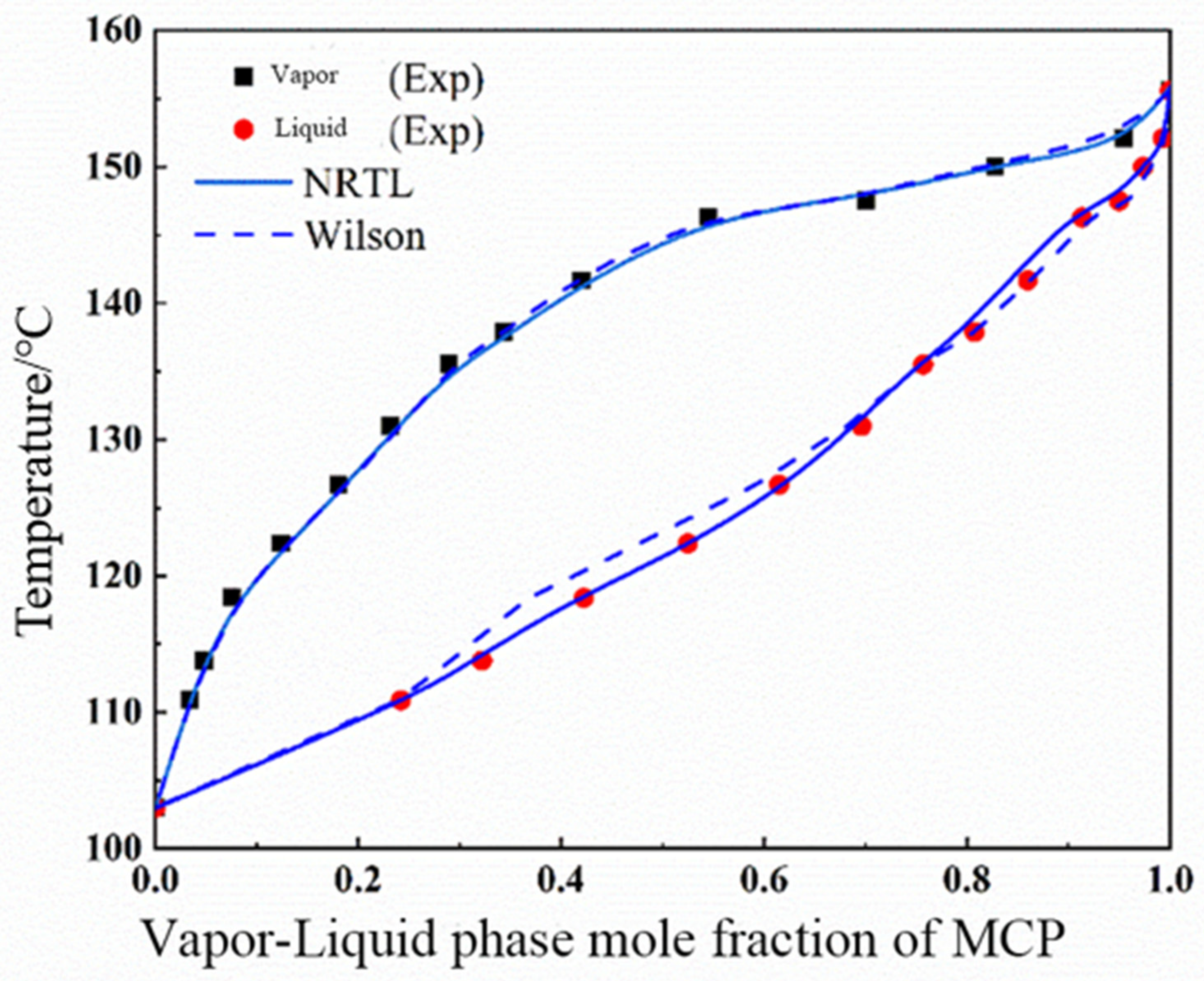
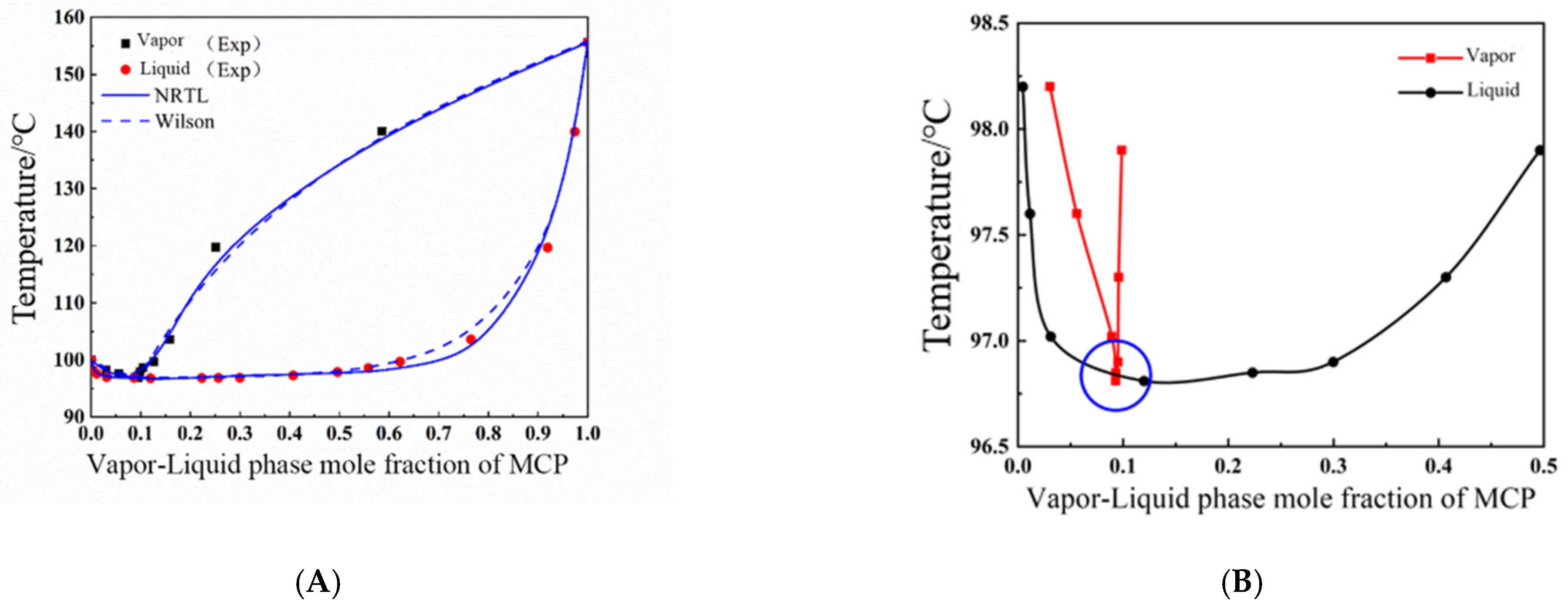
The theory of local composition suggests that the local composition of a solution is not equal to its overall composition. In a solution, the probability of other component atoms appearing around a certain component atom is influenced by the combination of component concentration and intermolecular interactions. The Wilson equation is the first equation established based on the local theory, in addition to the Non-Random Two Liquid (NRTL) equation applicable to partially miscible systems, as well as the Universal Mass Chemical Model (UNIQUAC) equation proposed based on the concept of local composition and lattice-like models.
In actual chemical production, there are often combinations between numerous components. It is unrealistic to measure the vapor–liquid equilibrium data of each multi-component system using experimental methods. The group contribution method is a phase-equilibrium estimation method. In the group contribution method, the physical properties of a mixture are obtained by the joint contribution of the groups that make up this system. In different systems, the contribution of the same group to the system is the same. The widely used group contribution-based equation is UNIQUAC (UNIQUAC functional group activity coefficients).
Due to the widespread application of local composition models, the brief introduction to their main equations is as follows:
(1)
Wilson equation [29]
The Wilson equation can accurately describe the activity coefficient in non-polar systems and polar miscible systems, especially in hydrocarbon alcohol systems, but the Wilson equation is not suitable for calculating the activity coefficient of partially miscible systems. The Wilson equation of binary systems is shown in Equations (3) and (4).
ln γ 1 = ln x 1 + Λ 12 x 2 + x 2 Λ 12 x 1 + Λ 12 x 2 Λ 21 x 2 + Λ 21 x 1
ln γ 2 = ln x 2 + Λ 21 x 1 + x 1 Λ 21 x 2 + Λ 21 x 1 Λ 12 x 1 + Λ 12 x 2
Based on the above equation, we obtain the following equation:
Λ ij = V j V i exp g i j g i i R T
In the above equation, Λij is the Wilson parameter, which is a dimensionless quantity, Λij > 0, and Λij ≠ Λji; however, Λi = Λj = 1. (gij-gji) is the energy parameter for the binary interaction, and gij = gji.
(2)
NRTL equation [30]
In 1968, Renon and Prausnitz further developed the concept of local composition, introducing non-random parameters that can reflect the characteristics of different components α12, and the NRTL equation was obtained. This equation can be used to calculate partially miscible systems, especially liquid–liquid layered systems. The NRTL equation is shown in Equation (7):
ln γ i = j τ j i G j i x j k G k i x k + j G i j x j k G k j x k τ i j l τ l j G l j x l k G k j x k
τ ji = g j i g i i R T
G ji = exp α j i τ j i
In the above equation, τij is the parameter of the NRTL equation; Gji is the interaction energy of the solution; αij is the characteristic function of the solution. Here, α is 0.3, and for most solutions, it is between 0.2 and 0.47.
(3)
UNIQUAC equation [31]
In 1975, Abrams and Prausnitz further introduced the size and shape parameters of molecules based on the quasilattice model and local composition model and derived the UNIQUAC equation using the double-liquid theory. Due to the introduction of molecular microscopic characteristic parameters, the equation theoretically has a wider range of applications, but currently, the microscopic parameters of some substances cannot be provided.
The UNIQUAC equation divides the activity coefficient into two parts, i.e., combination and remainder, which are used to reflect the molecular shape and the effect of shape, size, and intermolecular interaction on the activity coefficient. This equation is expressed as follows:
ln γ i = ln ϕ i x i + z 2 q i ln θ i ϕ i + l i ϕ i x i j x j l j q i ln j θ i τ j i + q i q i θ i τ j i k θ k τ k j
l i = z 2 ( r i q i ) r i 1
θ i = q i x i j q j x j
ϕ i = r i x i j r j x j
τ ij = exp u j i R T
In the above equation, θi and φi represent the average area fraction and volume fraction of pure substance i; ri and qi are pure material parameters calculated based on the van der Waals volume and surface area of the molecule; z is the lattice coordination number; uij is the interaction energy between molecules and i-j, determined using the experimental data.

3.4. Thermodynamic Consistency Verification

When measuring the complete vapor–liquid equilibrium data of a material system through experimental methods, errors cannot be completely avoided due to the influence of reagent purity, measuring instruments, system environment, and analytical detection. Therefore, it is necessary to use certain methods to determine whether the vapor–liquid equilibrium data of each group measured in the experiment are reliable. The Gibbs–Duhem equation shows that the activity coefficients of all components in the mixture are related to each other. If the activity coefficient of all components in the system can be measured, these data should comply with the Gibbs–Duhem equation. If a group of experimental data does not conform to the Gibbs–Duhem equation, it indicates that this group of data is incorrect and there is no correlation between the components. Instead, the method of using the activity coefficient form of the Gibbs–Duhem equation to check the quality of experimental data and whether the vapor–liquid two-phase data are related is called the thermodynamic consistency check of vapor–liquid equilibrium data.
For binary systems, the Gibbs–Duhem equation used for testing is in the following form:
x 1 dln γ 1 + x 2 dln γ 2 = V E R T d p H E R T 2 d T
The vapor–liquid equilibrium in this study is measured under constant-pressure conditions; therefore, dp = 0, and Equation (14) can be simplified as follows:
x 1 dln γ 1 + x 2 dln γ 2 = H E R T 2 d T
By integrating the above equation from x1 = 0 to x1 = 1, we conclude the following:
    x 1 = 0 x 1 = 1 l n γ 2 γ 1 d x 1 = x 1 = 0 x 1 = 1 H E R T 2 d T    
In the above equation, HE represents the excess mixing enthalpy, which usually varies with composition and temperature and is difficult to obtain experimentally. In 1947, Herington proposed a semi-empirical method based on the Gibbs–Duhem equation to perform consistency checks on the constant-pressure vapor–liquid equilibrium data of binary systems. The principle is to calculate the activity coefficients of each substance in the system from the experimental data and plot ln(γ12) versus x1. Then, we can calculate the value of D according to Equation (17). Using the maximum temperature Tmax and the minimum temperature Tmin of the system, J can be calculated according to Equation (18). If (D-J) < 10, it is considered that the constant-pressure vapor–liquid equilibrium data set is thermodynamically consistent.
  D = 100 × x 1 = 0 x 1 = 1 l n γ 1 / γ 2 d x 1 x 1 = 0 x 1 = 1 l n γ 1 / γ 2 d x 1     
J = 150 × T m a x T m i n T m i n
According to the phase-equilibrium criterion, when the two vapor and liquid phases reach equilibrium, where each component is i(i = 1, 2, ..., N), the fugacity in all directions is equal:
f i V = f i L
According to the definitions of fugacity and the fugacity coefficient, as well as activity and the activity coefficient, the fugacity of component i in the mixture can be expressed by the fugacity coefficient or by the activity coefficient. In the activity coefficient method, if the liquid fiL is expressed through the activity coefficient, then the following is true:
  P y i ϕ i f i V = f i θ x i γ i
In the above equation, fiθ represents the fugacity of component i in the standard state. According to the Lewis–Randall rule, the fugacity of the components in a mixture is equal to the fugacity of the pure liquid i at the equilibrium temperature T and pressure P; therefore, we obtain the following equation:
P y i ϕ i f i V = P i s i ϕ i S γ i x i e x p V i L P P i s R T                           
In Equation (21), P is the pressure under phase-equilibrium conditions; yi is the mole fraction of component i in the vapor phase; xi is the mole fraction of component i in the liquid phase; φiV is the fugacity coefficient in the vapor-phase mixture of component i; Pis is the saturated vapor pressure of pure substance i at phase-equilibrium temperature; φis is the fugacity coefficient of component i which is a pure gas at the equilibrium temperature T and saturated vapor pressure Pis; γi is the activity coefficient of component i; ViL is the liquid-phase molar volume of pure substance i.
When the system is at low pressure, the vapor phase can be regarded as an ideal gas. Equation (21) can be simplified as follows:
P y i = P i S γ i x i
The saturated vapor pressure in Equation (22) is usually calculated using the extended Antonie Equation (23), and Table 7 lists the parameters of the extended Antonie equation for each component. The Wagner equation is considered to be the most accurate and explicit functional equation for fitting experimental data. As it uses critical properties as parameters, the Wagner equation can more accurately describe the saturated vapor pressure data of most working fluids over a relatively large temperature range, even the data in the critical region [32]. In this section, the saturated vapor pressure of MCP is fitted using the Wagner equation, as shown in Equations (24) and (25). The parameters of the Wagner equation are in Table 8.
l n P i S = C 1 i + C 2 i T + C 3 i + C 4 i T + C 5 i l n T + C 6 i T C 7 i                                 
l n P i S = l n P c i + C 1 i 1 T r i + C 2 i 1 T r i 1.5 + C 3 i 1 T r i 2.5 + C 4 i 1 T r i 5 T r i            
T r i = T T c i
The integration test method is simple and easy to perform, but it is a comprehensive test of experimental data across the entire composition range. Therefore, there may be situations where the errors generated by different experimental points cancel out each other, causing the surface test to pass. If you want to identify “bad points” in the experimental data, you need to conduct point-by-point testing on all experimental data.
In 1973, Van Ness et al. proposed to use the △y value for point-by-point verification of the vapor–liquid equilibrium measurement results of a mixture system. The representative equation of △y is shown in Equation (26). If △y is less than 1, it indicates that the data have passed the test.
Δ y = i = 1 n 100 y i c a l y i e x p n

3.5. Verification Results of Thermodynamic Consistency

The post-calculation thermodynamic consistency verification results are shown in Table 9. From the table, it can be seen that the D-J values of the three binary systems are all less than 10, indicating that each group of data can pass the Herrington area test. Point tests were conducted according to the Wilson and NRTL equations, and the test results were all less than 1, indicating that the experimental data met the point test requirements. In summary, the vapor–liquid equilibrium data measured in this experiment at constant pressure all conform to thermodynamic consistency.

3.6. Correlation Results of Vapor–Liquid Equilibrium Data

The data measured in this experiment were regressed using the software Aspen Plus and the Wilson and NRTL activity coefficient equations for the constant-pressure vapor–liquid equilibrium data measured in the experiment. The regression operation defaults to using the maximum likelihood as the objective function to minimize the measurement errors of T, x, and y in the experiment. The maximum likelihood objective function expression is as follows:
Q = n w n m j x i j c a l x i j e x p σ x i 2 + j y i j c a l y i j e x p σ y i 2 + T i j c a l T e x p σ T i 2 + T i j c a l T e x p σ T i 2
The fitting results of activity coefficients of MCP–crotonaldehyde and MCP–water binary systems are shown in Table 10 and Table 11, respectively.
The average deviation (AAD) and root mean square deviation (RMSD) are used to describe the error analysis of correlation results. The calculation equations of AAD and RMSD are shown in Equations (28) and (29). It can be seen from Table 12 that the error between the temperature calculated by the Wilson and NRTL equations for MCP–crotonaldehyde and MCP–water binary systems and the experimental value is less than 0.15 °C. The error between the calculated vapor-phase MCP composition and the experimental values is less than 0.015. Therefore, both Wilson and NRTL equations are well correlated for these two binary systems.
A A D T = i = 1 n T i c a l T i e x p n
R M S D T = i = 1 n T i c a l T i e x p 2 n  

4. Process Simulation

4.1. Calculation Model Selection

For process simulation, the selection of thermodynamic models determines the accuracy and reliability of the calculation results and the success of the simulation. The commonly used thermodynamic models mainly include the equation of state model and the activity coefficient model. In process simulation, the available equation of state models are BWR-LS, PR, PSRK, RKS, etc., and the available activity coefficient models are Wilson, NRTL, UNIQUAC, UNIFAC, etc. The mixture system used in this study was a non-ideal mixture, and there were some intermiscible components in the system; thus, the NRTL-RK physical properties method was chosen. The boiling points and azeotropic compositions of the components of the mixture system at 101.325 kPa are shown in Table 13 [33] and Table 14 [33].

4.2. Simulation

The separation process of MCP and water was modeled using the software Aspen Plus v12.0. The thermodynamic model used in the simulation is NRTL, and the model parameters are listed in Table 12. Process parameters include initial fluid mass flow and temperature, distillation column pressure, MCP purity and component recovery, and water purity. Table 15 lists the values of these variables. Figure 5 illustrates the separation of MCP and water.
The rectification column T1 is used to concentrate the material in the feed; the top of the column is extracted from the azeotropes of crotonaldehyde and water and MCP and water; the liquid extracted from the top of the column is cooled to 45 °C in the decanter and divided into the oil phase and the water phase; the oil phase is passed into the rectification column T2 for further separation and purification; the product MCP is extracted from the T2 kettle; and crotonaldehyde and water azeotropes are extracted from the top of the column. Simulation results of atmospheric pressure separation of MCP from water in Table 16.

4.3. Simulation and Optimization of T1 Column

In this section, the theoretical number of trays and the kettle extraction of the T1 column were optimized using the mass flow of MCP in the kettle and the mass fraction of MCP at the top of the column as indicators.
(1) Theoretical plate number: As observed in Figure 6, the effectiveness of the separation increases with the number of trays in the rectification column, but the operating and equipment costs also increase. When the theoretical plate number is greater than 28, the curve becomes flatter. Therefore, it is recommended to choose the theoretical tray number of 28.
(2) Column kettle extraction: As observed in Figure 7, when the extraction of the column kettle is greater than 1368 kg/h, the MCP mass fraction at the top of the column decreases abruptly, and the MCP mass flow of the column kettle increases with the increase in the flow of the column kettle; thus, the extraction of the column kettle is set at 1350 kg/h.

4.4. Simulation and Optimization of T2 Column

In this section, the theoretical number of trays, feed positions, reflux ratios, and kettle extraction of the T2 tower were optimized using the kettle MCP mass fraction and the top-of-column MCP mass flow as indicators.
(1) Theoretical plate number: As observed in Figure 8, the effectiveness of the separation increases with the increase in the number of trays in the rectification column, but the operating and equipment costs also increase. When the number of theoretical trays is greater than eight, the curve becomes flatter. For this reason, the theoretical number of trays is chosen to be eight.
(2) Feed position: As observed in Figure 9, when the feed position is lower than the fifth tray, the kettle MCP mass fraction and the top-of-column MCP mass flow are nearly constant; thus, the third tray is selected as the feed position.
(3) Reflux ratio: As observed in Figure 10, the separation effect is obviously improved by increasing the reflux ratio. However, when the reflux ratio is increased to 0.1, the effect of reflux ratio on the separation effect gradually decreases. The reflux ratio is optimized to be 0.25.
(4) Column kettle extraction: As observed in Figure 11, when the extraction of the column kettle is greater than 303 kg/h, the MCP mass fraction of the column kettle and the mass flow of the MCP at the top of the column decrease and increase abruptly, respectively, from which the extraction of the column kettle is set to 303.1 kg/h.
The above sensitivity analyses of the main operating parameters affecting the process have been carried out; evidently, each influencing factor is not isolated, and the results of individual sensitivity analyses must be considered in conjunction with a comprehensive global analysis. The column operating conditions recommended by this study are shown in Table 17.

5. Conclusions

This study focuses on the vapor–liquid equilibrium data for MCP–crotonaldehyde and MCP–water measured using a modified Rose–Williams equilibrium instrument and the obtained T-x-y phase diagrams. The thermodynamic consistency of the experimental data was verified using the Herrington area and Van Ness point tests. It was found that MCP and water formed the lowest azeotrope at 102 kPa with an azeotropic temperature of 96.8 °C. The mole fraction of water in this azeotrope was 90.9% and that of MCP was 9.1%. The experimental data were regressed using the Wilson and NRTL activity coefficient equations to derive the binary interaction parameters for each equation. The calculated values for both equations were in good agreement with the experimental values. The NRTL-RK model was selected to simulate the process for recovering and purifying MCP. A sensitivity analysis for the influencing factors of the atmospheric pressure rectification column was performed. A two-column process was developed and optimized in this study, and the aim of effectively utilizing the by-product MCP was achieved with this process.

Author Contributions

Data Curation: Y.B.; Formal analysis: Y.B.; Funding acquisition: Z.G.; Investigation: Z.G.; Methodology: Y.B.; Project administration: F.S.; Supervision: K.Z.; Validation: F.S.; Visualization: Y.B.; Writing-original draft: Y.B.; Writing-review & editing: Y.B. All authors have read and agreed to the published version of the manuscript.

Funding

This research received no external funding.

Data Availability Statement

Data unavailability due to privacy or ethical constraints.

Acknowledgments

This study was supported by the National Natural Science Foundation of China (Grant No. 21978199).

Conflicts of Interest

Author Feng Shi was employed by the company Tianjin Jiuyuan Chemical Engineering Co. Ltd. The remaining authors declare that the re-search was con-ducted in the absence of any commercial or financial relationships that could be construed as a potential conflict of interest.

References

  1. Liu, T.; Chen, X.; Jiang, R. A review on the mechanism of action, toxicity and detection methods of potassium sorbate. Mod. Food 2020, 18, 96–98. [Google Scholar] [CrossRef]
  2. Chen, R.; Kang, S.; Gao, Y.; Huang, M.; Zheng, Y. Progress in the preparation of crotonic acid and its application. Fine Pet. Chem. 2021, 38, 75–81. [Google Scholar]
  3. Wu, H.; Zhang, S.; Li, D.; Pang, Y.; Sun, J.; Li, Y. Application of sorbic acid and its potassium salts in food. Agric. Sci. Inf. 2023, 07, 149–152. [Google Scholar] [CrossRef]
  4. Liu, T. Study on the Toxicity Reduction Process of Biological Treatment of Wastewater from Crotonaldehyde Production. Master’s Thesis, Lanzhou Jiaotong University, Lanzhou, China, 2020. [Google Scholar]
  5. Zhang, M.H.; Guan, X.Y.; Zhuang, J.Y.; Yu, Y.Z. Insights into the mechanism of ethanol conversion into 1,3-butadiene on Zr-β zeolite. Appl. Surf. Sci. 2022, 579, 152212. [Google Scholar] [CrossRef]
  6. Li, F.; Wang, H.; Chen, S.; Li, W.; Cui, X.; Li, R. Preparation of Zr-Beta with different structures and the performance of MPV reaction. Appl. Chem. Ind. 2020, 49, 867. [Google Scholar]
  7. Yu, Q.; Guo, Y.; Wu, X.; Yang, Z.; Wang, H.; Ge, Q.; Zhu, X. Ketonization of propionic acid on Lewis acidic Zr-beta zeolite with improved stability and selectivity. ACS Sustain. Chem. Eng. 2021, 9, 7982–7992. [Google Scholar] [CrossRef]
  8. Zhang, M.; Yang, G.; Wang, L.; Jiang, H. Heteroatom Beta Molecular Sieve Useful for Aldol Condensation of Low-Carbon Aldehyde, Comprises E.G. Titanium, Tin, Zirconium, Tantalum, Cerium, Hafnium, Yttrium, Niobium, Vanadium, Zinc, Scandium and Iron. CN115947349-A, 11 April 2023. [Google Scholar]
  9. Zhao, Y. Preparation of Zr-β Molecular Sieves and their Catalytic Performance in the Production of crotonaldehyde from Acetaldehyde. Master’s Thesis, Tianjin University, Tianjin, China, 2022. [Google Scholar]
  10. Kong, D. Preparation of Zr-β Heteroatomic Molecular Sieves and Their Catalytic Study of Ethanol-Acetaldehyde to Butadiene Production. Master’s Thesis, Tianjin University, Tianjin, China, 2021. [Google Scholar]
  11. Zhang, M.; Yang, G.; Wang, L.; Jiang, H. Hierarchically Porous Beta Molecular Sieve with Beta Polymorph A Structure Useful for Catalyzing Aldol Condensation of Acetaldehyde to Prepare Crotonaldehyde and Subjecting to Meerwein-Ponndorf-Verley Catalytic Reaction to Prepare Crotyl Alcohol, Comprises Microporous and Mesoporous Structure. CN114835136-A, 2 August 2022. [Google Scholar]
  12. Chen, Y.; Zhang, G.; Ye, Y.; Wang, H. Determination and correlation of vapor-liquid equilibrium of hexanoic acid + acetic acid/butyl acetate/cyclohexanone/ε-caprolactone system at 20 kPa. Chem. Eng. 2021, 49, 42–47. [Google Scholar]
  13. Wang, Z. Study on the Phase Equilibria of the systems in Acromatic Extraction Process with N-Formylmorpholine as Solvent. Master’s Thesis, Tianjin University, Tianjin, China, 2013. [Google Scholar]
  14. Li, P. Study on Vapor-Liquid Equilibrium of Methanol-Formaldehyde-Polyoxymethylene Dimethyl Ethers. Master’s Thesis, China University of Petroleum, Dongying, China, 2021. [Google Scholar]
  15. Zhao, J.; Tan, Z.; Guo, X.; Jin, C. Determination and correlation of phase equilibrium about methanol-n-butanol at atmospheric pressure. Chem. Eng. 2020, 48, 53. [Google Scholar]
  16. Zhao, J.; Tan, Z.; Meng, X.; Li, C.; Tong, Z. Determination and correlation of methanol-ethanol phase equilibria at atmospheric pressure. Nat. Gas Chem. 2021, 46, 71–75. [Google Scholar]
  17. Li, J.; Yang, X.; Jiang, W.; Tang, S.; Tian, W. Experiments on phase equilibria and model regression of activity coefficients for binary azeotropes. Exp. Sci. Technol. 2021, 19, 65–68. [Google Scholar]
  18. Fornari, R.E.; Alessi, P.; Kikic, I. High pressure fluid phase equilibria: Experimental methods and systems investigated (1978–1987). Fluid Phase Equilibria 1990, 57, 1–33. [Google Scholar] [CrossRef]
  19. Rogalski, M.; Rybakiewicz, K.; Malanowski, S. Rapid and Accurate Method for Determination of Vapour-Liquid Equilibrium. Berichte Bunsenges. Phys. Chem. 1977, 81, 1070–1073. [Google Scholar] [CrossRef]
  20. Malanowski, S. Experimental methods for vapour-liquid equilibria. Part I. Circulation methods. Fluid Phase Equilibria 1982, 8, 197–219. [Google Scholar] [CrossRef]
  21. Yang, H.J. Study on the Separation of Ethanol-Water System by a New Azeotropic Distillation Water Splitting Technique. Master’s Thesis, Tianjin University, Tianjin, China, 2006. [Google Scholar]
  22. Liu, W.S.; Jiao, Z.L.; Ma, S.B.; Liu, W.; Huang, M.S.; Liu, H. Vacuum distillation for impurity separation and purification of scandium metal. Rare Met. Cem. Carbides 2025, 53, 12–17. [Google Scholar]
  23. Zhao, A.; Guo, H. Improvement of experiments for the determination of binary vapor-liquid equilibrium data. Lab. Sci. 2019, 22, 45–48. [Google Scholar]
  24. Łenka, M.; Persson, O.; Rasmussen, P. A modified Dvořak-Boublík (vapour + liquid) recirculating still with continuous analysis of the compositions of phases. J. Chem. Thermodyn. 1991, 23, 851–858. [Google Scholar] [CrossRef]
  25. Hao, Y.; Zhang, S.; Yao, K. Vapor–liquid equilibrium data for methanol+tert-butylamine+n, n-dimethylformamide and constituent binary systems at atmospheric pressure. J. Chem. Eng. Data 2012, 57, 1244–1248. [Google Scholar] [CrossRef]
  26. Yazdizadeh, M.; Eslamimanesh, A.; Esmaeilzadeh, F. Applications of cubic equations of state for determination of the solubilities of industrial solid compounds in supercritical carbon dioxide: A comparative study. Chem. Eng. Sci. 2012, 71, 283–299. [Google Scholar] [CrossRef]
  27. Peng, J.; Tian, G.; Liu, Y. Selection and application of equations of state for high-pressure natural gas. Gas Heat 2004, 24, 481–485. [Google Scholar]
  28. Hou, Y.; Chen, X.; Zhou, H. Martin-Howe equation of state toward the solid phase. J. Chem. Eng. High. Educ. 1996, 10, 2–9. [Google Scholar]
  29. Wilson, G.M. Vapor-liquid equilibrium. XI. A new expression for the excess free energy of mixing. J. Am. Chem. Soc. 1964, 86, 127–130. [Google Scholar] [CrossRef]
  30. Renon, H.; Prausnitz, J.M. Local compositions in thermodynamic excess functions for liquid mixtures. AIChE J. 1968, 14, 135–144. [Google Scholar] [CrossRef]
  31. Abrams, D.S.; Prausnitz, J.M. Statistical thermodynamics of liquid mixtures: A new expression for the excess Gibbs energy of partly or completely miscible systems. AIChE J. 1975, 21, 116–128. [Google Scholar] [CrossRef]
  32. Wang, G. Sorbic acid production key process discussion. Meat Res. 2011, 25, 66–72. [Google Scholar]
  33. Geng, Z.; Sheng, L.; Zhang, K.; Shi, F.; Gong, H. Study on the process of producing crotonaldehyde from acetaldehyde catalyzed by Zr-β zeolite. Sep. Purif. Technol. 2024, 335, 126123. [Google Scholar] [CrossRef]
Figure 1. Schematic diagram of small vapor–liquid balancing kettle. 1—condenser; 2—vapor-phase liquid extraction port; 3—vapor-phase storage tank; 4—crossover pipe; 5—buffer ball; 6—elevator pipe; 7—return pipe; 8—heating rod; 9—boiling chamber; 10—liquid-phase extraction port; 11—liquid-phase storage tank; 12—balance chamber; 13—bell jar; 14—vacuum jacket; 15—thermometer well.
Processes 13 01435 g001
Figure 2. Comparison of VLE data of methanol (1)–isopropanol (2) with those reported in the literature: Ref. 1 [24] and Ref. 2 [25].
Processes 13 01435 g002
Figure 3. T-x-y phase diagram for MCP (1)–crotonaldehyde (2) system at 102 kPa.
Processes 13 01435 g003
Figure 4. (A) T-x-y phase diagram for MCP (1)–water (2) system at 102 kPa; (B) representation of partial enlargement of azeotropic point of MCP and water.
Processes 13 01435 g004
Figure 5. Aspen Plus process flow diagram (PFD) of azeotropic distillation sequence.
Processes 13 01435 g005
Figure 6. Effect of theoretical tray number of T1 column.
Processes 13 01435 g006
Figure 7. Effect of T1 column kettle extraction.
Processes 13 01435 g007
Figure 8. Effect of theoretical tray number in T2 column.
Processes 13 01435 g008
Figure 9. Effect of T2 column feed position.
Processes 13 01435 g009
Figure 10. Effect of reflux ratio of T2 column.
Processes 13 01435 g010
Figure 11. Effect of T2 column kettle extraction.
Processes 13 01435 g011
Table 1. List of reagents used in experiment.
Reagent NameCAS
Number
Molecular MassPurity SpecificationsManufacturer
Methanol67-56-132.04>99.5; ARAladdin reagent, Tokyo, Japan
Isopropanol67-63-060.01ACS > 99.5%Aladdin reagent
2-Methyl-2-cyclopentene-1-one1120-73-696.13>97%; GCAladdin reagent
Crotonaldehyde4170-30-370.09>98%; ARMaclean’s reagent, Toronto, ON, Canada
Deionized water7732-18-518.015———Made in our laboratory
Table 2. List of instruments used in experiment.
Instrument NameSpecificationManufacturer
Gas Chromatography-Mass SpectrometerShimadzu GCMS-QP2020 NXSHIMADZU, Chiyoda, Japan
Gas chromatographShimadzu GC-2010SHIMADZU
Second-class standard mercury thermometer1/10Wuqiang County Zhongxing Glassware Factory, Hengshui, China
TDGCTDGC2-1kVAGreat Wall Electric Appliance Group Co., Ltd., Suzhou, China
Cold water bathMPG-20CShanghai Yiheng Scientific Instruments Co., Ltd., Shanghai, China
Vapor–liquid equilibrium kettleMade by Tianjin University
Table 3. Results of relative correction factor.
Substance 1Substance 2
Methanol (1)–isopropanol (2)10.6425
MCP (1)–crotonaldehyde (2)11.2574
MCP (1)–water (2)10.6584
Table 4. VLE data for methanol (1)–isopropanol (2) system at 102 kPa.
T/°Cx1y1x2y2
81.850.00000.00001.00001.0000
78.470.27980.17640.72020.8236
78.100.32020.19930.67980.8007
77.700.34460.21920.65540.7808
77.000.41420.26680.58580.7332
76.000.46930.30850.53070.6915
73.720.62840.46070.37160.5393
72.920.66830.49880.33170.5012
70.300.79520.63110.20480.3689
69.320.83140.68510.16860.3149
68.400.86510.73610.13490.2639
67.700.89050.78180.10950.2182
67.230.91050.81180.08950.1882
65.020.98070.95510.01930.0449
64.420.99780.99470.00220.0053
64.500.99490.98790.00510.0121
Table 5. VLE data for MCP (1)–crotonaldehyde (2) system at 102 kPa.
T/°Cx1y1x2y2
155.601.00001.00000.00000.0000
152.100.99290.95460.00710.0454
150.000.97360.82840.02640.1716
147.500.94980.70070.05020.2993
146.300.91340.54540.08660.4546
141.700.85990.42070.14010.5793
137.900.80730.34410.19270.6559
135.520.75670.28970.24330.7103
131.000.69610.23200.30390.7680
126.700.61490.18060.38510.8194
122.400.52490.12370.47510.8763
118.400.42220.07600.57780.9240
113.800.32230.04850.67770.9515
110.900.24220.03420.75780.9658
103.000.00000.00001.00001.0000
Table 6. VLE data for MCP (1)–water (2) system at 102 kPa.
T/°Cx1y1x2y2
155.601.00001.00000.00000.0000
140.000.97410.58600.02590.4140
119.700.91930.25090.08070.7491
103.600.76500.15920.23500.8408
99.700.62210.12630.37790.8737
98.600.55850.10450.44150.8955
97.900.49630.09870.50370.9013
97.300.40690.09570.59310.9043
96.900.29970.09510.70030.9049
96.870.25650.09380.74350.9062
96.850.22300.09310.77700.9069
96.810.11980.09290.88020.9071
96.900.08620.09220.91380.9078
97.020.03120.08930.96880.9107
97.600.01140.05600.98860.9440
98.200.00450.03040.99550.9696
100.000.00000.00001.00001.0000
Table 7. Parameters of extended Antonie equation.
SubstanceC1iC2iC3iC4iC5iC6iC7iC8i/KC9i/K
Methanol75.81−6904.5000−8.867.47 × 10−62175.47512.50
Isopropanol103.81−9040.0000−12.685.54 × 10−62185.26508.30
Crotonaldehyde73.15−7159.8000−8.352.24 × 10−176196.65565.00
Water66.74−7258.2000−7.304.16 × 10−62273.16647.10
Table 8. Parameters of Wagner equation.
SubstanceC1iC2iC3iC4iC5iC6iC7iC8i/K
MCP−7.932.04−3.19−3.388.43654200654
Table 9. Results of thermodynamic consistency test.
SystemSurface InspectionPoint InspectionResult
DJD-J△y a△y b
Methanol (1)–isopropanol (2)15.167.717.450.14890.1178Pass
MCP (1)–crotonaldehyde (2)27.1120.976.140.73090.0739Pass
MCP (1)–water (2)−1.8622.35−24.210.79590.4427Pass
a Calculation results of Wilson equation; b calculation results of NRTL equation.
Table 10. Results of NRTL and Wilson equation fitting for MCP–crotonaldehyde system.
T/°Cx1Expy1Expx1Wilsony1Wilsonx1NRTLy1NRTL
155.601.0000 1.0000 1.0000 1.0000 1.0000 1.0000
152.100.9929 0.9546 0.9959 0.9476 0.9941 0.9543
150.000.9736 0.8284 0.9813 0.8094 0.9741 0.8282
147.500.9498 0.7007 0.9595 0.6784 0.9464 0.7014
146.300.9134 0.5454 0.9230 0.5330 0.9016 0.5498
141.700.8599 0.4207 0.8620 0.4113 0.8408 0.4233
137.900.8073 0.3441 0.8072 0.3447 0.7882 0.3456
135.520.75670.28970.7545 0.2933 0.7432 0.2906
131.000.6961 0.2320 0.6821 0.2428 0.6803 0.2326
126.700.6149 0.1806 0.5925 0.1891 0.6105 0.1808
122.400.5249 0.1237 0.4771 0.1301 0.5124 0.1239
118.400.4222 0.0760 0.3669 0.0823 0.3961 0.0761
113.800.3223 0.0485 0.2894 0.0518 0.3032 0.0486
110.900.2422 0.0342 0.2392 0.0345 0.2472 0.0342
103.000.0000 0.0000 0.0000 0.0000 0.0000 0.0000
Table 11. Results of NRTL and Wilson equation fitting for MCP–crotonaldehyde system.
T/°Cx1Expy1Expx1Wilsony1Wilsonx1NRTLy1NRTL
155.60 1.0000 1.0000 1.0000 1.0000 1.0000 1.0000
140.00 0.9741 0.5860 0.9740 0.5691 0.9744 0.5833
119.70 0.9193 0.2509 0.9196 0.2756 0.9177 0.2521
103.60 0.7650 0.1592 0.7662 0.1419 0.7996 0.1548
99.70 0.6221 0.1263 0.6222 0.1175 0.7085 0.1204
98.60 0.5585 0.1045 0.5560 0.1120 0.6208 0.1025
97.90 0.4963 0.0987 0.4943 0.1084 0.5738 0.0944
97.30 0.4069 0.0957 0.4059 0.1047 0.4452 0.0846
96.90 0.2997 0.0951 0.2994 0.1016 0.2584 0.0870
96.87 0.2565 0.0938 0.2563 0.1006 0.2320 0.0898
96.85 0.2230 0.0931 0.2229 0.0998 0.2148 0.0917
96.81 0.1198 0.0929 0.1198 0.0972 0.1362 0.1028
96.90 0.0862 0.0922 0.0862 0.0957 0.0844 0.1070
97.02 0.0312 0.0893 0.0312 0.0853 0.0351 0.0868
97.60 0.0114 0.0560 0.0113 0.0613 0.0156 0.0535
98.20 0.0045 0.0304 0.0045 0.0349 0.0073 0.0287
100.00 0.0000 0.0000 0.0000 0.0000 0.0000 0.0000
Table 12. Summary of model regression parameter results.
ParameterWilsonNRTL
MCP (1)–crotonaldehyde (2)
aij−22.4415.54
aji−15.5435.08
bij−7263.99−6715.35
bji6544.99−12,079.21
αij 0.3
AAD(T/°C)0.02280.0040
RMSD(T/°C)0.03930.0048
AAD(y1)0.00730.0008
RMSD(y1)0.00980.0014
MCP (1)–water (2)
aij13.8016.45
aji2.08−30.66
bij−6473.52−6053.66
bji−1178.2912,604.80
αij 0.3
AAD(T/°C)0.10030.0231
RMSD(T/°C)0.11660.0329
AAD(y1)0.00800.0045
RMSD(y1)0.01010.0060
Table 13. Boiling points of pure components in studied system.
ComponentBoiling Point/°CMolecular Mass
Acetaldehyde20.544.0
Ethyl acetate77.288.1
Ethanol78.346.1
Water100.018.0
Crotonaldehyde104.070.1
Acetic acid118.060.1
MCP158.096.1
Sorbic acid228.0112.1
Table 14. Azeotropic point and azeotropic composition of azeotropes in studied system.
AzeotropeAzeotropic Point/°CAzeotropic Composition/wt% *
Ethyl acetate–water70.491.53–8.47%
Ethyl acetate–ethanol71.870.2–29.8%
Crotonaldehyde–ethanol–water78.07.3–87.9–4.8%
Ethanol–water78.296–4%
Crotonaldehyde–water84.075.7–24.3%
MCP–water96.834.8–65.2%
* Data source: Azeotropic Data-III.
Table 15. Specification of design variables in azeotropic distillation process.
VariableSpecification
Feed stream
Temperature (°C)91.51
Mass flow (kg/h)3253.23
MCP mass fraction0.09
Decanter
Temperature (°C)45
Purity (water mass fraction)0.96
Azeotropic column T2
Operation pressure (kPa)101.3
Purity (MCP mass fraction)0.99
Recovery of MCP (%)99.9
Table 16. Simulation results for atmospheric pressure separation of MCP–water.
ItemsFeed11216119MCP
Temperature (°C)91.5102.64589.3168.9
Pressure (bar)4.14.11.14.14.1
Mass flow (kg/h)325313501201898303
Water0.720.990.260.350.0001
MCP0.090.00010.250.00010.999
Table 17. Optimal process parameters for columns T1 and T2.
Rectification Column T1Rectification Column T2
Theoretical tray number288
Feed position 3
Reflux ratio 0.25
Column kettle extraction (kg/h)1350303.1
Disclaimer/Publisher’s Note: The statements, opinions and data contained in all publications are solely those of the individual author(s) and contributor(s) and not of MDPI and/or the editor(s). MDPI and/or the editor(s) disclaim responsibility for any injury to people or property resulting from any ideas, methods, instructions or products referred to in the content.

