Article

Revision of the Screening Robust Estimation Method for the Retrospective Analysis of Normal Processes

by
Víctor H. Morales
1,*,†,
Carlos A. Panza
2,† and
Roberto J. Herrera
3,†
1
Departamento de Matemáticas y Estadística, Universidad de Córdoba, Montería 230027, Colombia
2
Departamento de Estadística, Universidad Nacional de Colombia, Bogotá 110221, Colombia
3
Departamento de Ingenieía Industrial, Universidad del Atlántico, Barranquilla 111321, Colombia
*
Author to whom correspondence should be addressed.
All authors contributed equally to this work.
Processes 2025, 13(5), 1381; https://doi.org/10.3390/pr13051381
Submission received: 16 March 2025 / Revised: 12 April 2025 / Accepted: 17 April 2025 / Published: 30 April 2025

Abstract

:
This paper provides a comprehensive review of the Screening Robust Estimation Method (SREM) for normal processes in Phase I. Particular emphasis is placed on the exponentially weighted moving average (EWMA) control chart, which is employed in the retrospective monitoring stage. A central concern addressed in this discussion is that the EWMA chart is said to be based on the false alarm rate (FAR) design criterion, but it is accurately implemented. It is well established that FAR-based methods for Phase I monitoring assume that the distribution of the monitoring statistic remains invariant at each sampling instance. However, the EWMA statistic inherently introduces a sequential dependence among all sampling moments, which contradicts this assumption. This paper shows that a modified EWMA chart, incorporating probability-based control limits rather than the conventional formulation utilized in the SREM, enhances the monitoring of normal processes in Phase I. Through simulations, it is established that the new design proposal of an EWMA chart for Phase I monitoring has a slightly narrower decision threshold among the control methodologies included in the study. The new chart is as effective as the traditional X ¯ charts in detecting localized increases in the target value of the mean of a normal process, and outperforms them when other types of anomalies are present in the available preliminary samples.

1. Introduction

In contemporary statistical quality control (SQC) practices, process improvement initiatives in both production and service operations frequently incorporate procedures for designing control charts to facilitate monitoring. There are two stages of analysis, often referred to as the retrospective (Phase I) and prospective (Phase II) phases, both of which depend considerably on control chart design. Phase I analysis serves an exploratory function, involving the application of statistical methods and techniques to gain insights into patterns in process performance and variation. Once process stability is established by identifying and addressing anomalous observations, an appropriate model is developed and estimated using the remaining data. In contrast, the primary objective of Phase II monitoring is to promptly detect deviations from the assumed stable model.
A comprehensive Phase I analysis should extend beyond simply designing a control scheme for establishing the stability of the available data. The effectiveness of online process monitoring in the prospective stage is highly dependent on the rigor and accuracy of the retrospective analysis. Consequently, several researchers have emphasized the importance of establishing precise control limits in both the retrospective and the prospective stages of monitoring. Jensen et al. [1] provide an overview of the effect of parameter estimation on the performance of Phase II control charts. Chakraborti et al. [2] provide a detailed review with key technical insights on the determination of control limits for univariate control charts in Phase I. Additionally, Jones-Farmer et al. [3] present a less technical review that considers control chart design and other Phase I methodologies for both univariate and multivariate processes, including profile monitoring. The authors also identify potential avenues for further research in Phase I quality control.
The present article reviews and discusses the Screening Robust Estimation Method (SREM) proposed by Zwetsloot et al. [4]. Originally introduced as a method for detecting various data anomalies in the target value of a normally distributed process in Phase I analysis, the SREM seeks to mitigate the need for developing new control procedures which incorporate robust estimation methods for the unknown parameters of a basic model that characterizes the quality of univariate processes, as suggested by Jones-Farmer et al. [3]. The SREM also aligns with the need to establish accurate control limits, as described in Chakraborti et al. [2]. The SREM also involves the novel idea of using EWMA schemes in Phase I as well for monitoring purposes. EWMA charts were first proposed by Roberts [5], and have been shown to be exclusively effective in monitoring processes in prospective Phase II.
Rather than employing the EWMA statistic as initially specified in the SREM, we propose extending the use of the EWMA chart with dynamic probability limits in Phase II, as introduced by Shen et al. [6], to Phase I analysis. Through simulation studies, it will be shown that the EWMA chart within the SREM framework is not accurately designed. Instead of designing the EWMA chart in the SREM as is originally suggested in Zwetsloot et al. [4], we propose adapting the simulation-based algorithm presented in Shen et al. [6] to estimate the decision threshold of the EWMA chart for Phase I using probability limits. Our results illustrate that the proposed adaptation of the probability limit approach to Phase I retrospective analysis can enhance the methodology developed by Zwetsloot et al. [4].
The central focus of our discussion is the claim made in the original formulation of the EWMA chart presented in the SREM, which asserts that it constitutes a control methodology governed by a predefined false alarm rate (FAR). Upon closer examination, this claim proves to be inaccurate. FAR-based control methods rely on the assumption that the distribution of the charting statistic is independent from the monitoring instance. However, the EWMA statistic inherently generates a control scheme that is sequentially dependent. This critical problem was not accounted for in the design proposed by Zwetsloot et al. [4]. To rectify this, we propose a probability-limit-based framework which aims to address the inaccuracies introduced in the monitoring of normal processes by the original EWMA chart design of the SREM.
The remainder of this article is structured as follows. Section 2 presents the theoretical framework motivating the revision of the SREM. Section 3 details the simulation study conducted, while the key findings are highlighted in Section 4. Finally, Section 5 and Section 6 provide a simulated example, along with concluding remarks and recommendations for future research directions.

2. Theoretical Background

2.1. Some General Features of Phase I Analysis

Let X N ( μ , σ 2 ) be the random variable that characterizes the quality of a process. The central problem concerning the monitoring of the mean μ of the process under consideration can be formally posed by testing the statistical hypotheses given at different time points t as follows:
H 0 : μ t = μ 0 H 1 : μ t = μ 1 ,
where μ 0 and μ 1 are, respectively, the target in-control and out-of-control values of the process mean μ . That is, the mean of the process remains at its target value or shifts from it at instance t.
To verify process stability according to the hypothesis test stated in (1), control charts are traditionally used in both Phase I and Phase II. One example of these procedures is the X ¯ chart, which monitors the mean value of a process over time and helps detect any shifts from the target value. This section addresses key issues discussed in Chakraborti et al. [2], as they form the foundation of the present discussion, especially in Phase I. According to these authors, the retrospective stage of monitoring presents a decision problem similar to that of testing the homogeneity of a finite number of data groups.
Let k > 1 denote the number of independent samples of size n > 1 , taken from some continuous random variable X characterizing process quality. A control scheme consists of the charting statistics C t , t = 1 , , k , and some control limits that are functions of the estimated parameter vector defining the distribution of X. Once the control chart is designed, the evaluation of process stability is begun. The iterative Phase I control procedure is outlined in its entirety in Montgomery [7]. A signal indicating a potential out-of-control situation occurs when at least one charting statistic exceeds the most recently calculated control limits.
Chakraborti et al. [2] identify two primary approaches for establishing control limits in Phase I analysis. The first approach, originally proposed by Hillier [8] and Yang and Hillier [9], determines control limits by maintaining the false alarm rate (FAR) at a specified level. The FAR is defined as the probability of a false alarm for each of the k available samples and relies solely on the knowledge of the marginal distribution of the tth charting statistic C t , t = 1 , , k . However, this approach does not take into account the simultaneous comparison of several data subgroups against the same control limits. As previously established, this approach has been shown to substantially increase the nominal FAR level.
On the other hand, the second approach proposes evaluating the control limits for a previously specified false alarm probability (FAPr), defined as the overall probability of at least one false alarm among the available k data subgroups. The FAPr can be expressed as
F A P r = 1 P t = 1 k E t I C = a b a b f C 1 , , C k ( c 1 , , c k ) d c 1 d c k ,
where f C 1 , , C k ( c 1 , , c k ) is the joint probability density function of the charting statistics C t , t = 1 , , k when the process is in control, and a and b are the control limits. Clearly, the calculation of the FAPr involves the simultaneity of k statistically dependent, nonsignaling events. This approach, first proposed by King [10], has emerged as the most commonly recommended criterion for control chart design in Phase I.
Nevertheless, the derivation of the joint distribution f C 1 , , C k ( c 1 , , c k ) and the subsequent evaluation of the control limits a and b in (2) may represent a cumbersome task. Some approximated methodologies have been proposed to avoid the need for knowledge of the joint distribution of the charting statistics. For more details, see Chakraborti et al. [2].

2.2. The EWMA-Based Screening Robust Estimation Method

Let X i t denote the ith observation, i = 1 , 2 , , n of the tth sample, t = 1 , 2 , , k . It is assumed that all X i t observations are independently and identically normally distributed with the mean μ and standard deviation σ when the process is in control. Zwetsloot et al. [4] explored some monitoring methods based on robust estimators of the normal location and scale parameters, μ and σ , as well as the efficient X ¯ ¯ estimator for Phase I analysis. The authors specifically focused on monitoring methods based on the conventional formulation of the EWMA statistic. They recommended the use of a Phase I EWMA chart with λ I = 0.6 (or a similar intermediate value) based on the robust estimator of the location parameter, rather than on the efficient estimator. In their study, the value of k was set to 50, and n was set to 5 or 10.
The Phase I EWMA-based screening estimation procedure is implemented as follows. First, initial estimates of the mean and the standard deviation, μ ^ and σ ^ , respectively, are required. The method for obtaining these estimates is presented below. Next, for the tth sampling moment, t = 1 , , k , the Phase I EWMA charting statistic is defined as
Z t = λ I X ¯ t + ( 1 λ I ) Z t 1 ,
with control limits
μ ^ + L σ ^ λ I 1 ( 1 λ I ) 2 t n ( 2 λ I ) ,
where Z 0 = μ ^ , and 0 < λ I 1 is the smoothing constant of the EWMA statistic in Phase I. If Z t falls beyond the control limits for a given monitoring instance t, the corresponding sample is identified as unacceptable and deleted from the analysis.
The initial estimate of the normal mean is proposed to be the median of the available k sample averages, M ( X ¯ ) ; this is
μ ^ = M ( X ¯ ) = med ( X ¯ 1 , , X ¯ k ) .
Janacek and Meikle [11] found that this estimate is efficient and robust against various data anomalies. The process standard deviation estimate σ ^ is set to be a variant of the bi-weight A estimator proposed by Tatum [12], which is renowned for its robustness. The estimation procedure is outlined in Tatum [12] and was implemented as described in Schoonhoven et al. [13] with normalizing constants of d = 1.068 for n = 5 and d = 0.962 for n = 10 .
Given the prevalence of various types of outliers in Phase I data, which are typically not known in advance, the design of control charts based on robust estimators is a recommended approach. For a comprehensive discussion on robust estimation in univariate Phase I data, see Rocke [14], Graham et al. [15], Schoonhoven et al. [16] and Schoonhoven and Does [17,18]. Nazir et al. [19] apply robust point location estimators for designing CUSUM charts in Phase II. In the context of multivariate process monitoring, Vargas [20], Jensen et al. [21], Oyeyimi & Ipinyomi [22], and Yañez et al. [23] propose control methodologies that incorporate robust estimators of the normal covariance matrix in Phase I. Ahmadi and Shahriari [24] propose the monitoring of simple linear profiles using robust M-estimators of the basic model error term variance. Neto et al. [25] consider robust regression techniques in the design of Shewhart-type control charts.
Another important aspect of control chart design is the selection of the constant L in (4). The corresponding values for L were originally obtained through simulation and were intended to align with the recommendations in Chakraborti et al. [2]. However, as will be discussed later, these recommendations were not followed. According to Zwetsloot et al. [4], necessary L values were computed for all possible combinations of smoothing constants λ I = 0.2 , 0.6 , and 1.0 and sample sizes n = 5 and 10 in the case of standard normal observations. All monitoring methods explored were calibrated to achieve a nominal FAR level of 1 % .

2.3. Critique of the SREM

The primary critique of the SREM concerns the procedure used to determine the control limits. After obtaining robust estimates for the normal mean and standard deviation, the SREM aims to calculate the value of the constant L in Equation (4) that satisfies a predetermined FAR level, in accordance with the recommendations in Chakraborti et al. [2]. However, these recommendations were not adhered to in practice. It would have been more appropriate for the control limits to have been computed based on the marginal distribution of the EWMA statistic at each monitoring instance, particularly if the method were intended to be FAR-based.
Recall that EWMA charts with λ 1 violate the assumption about the independence of the charting statistics. In our view, the application of EWMA-based charts in Phase I monitoring presents a more complex challenge compared to other screening methods, such as Phase I Shewhart-type schemes. Specifically, it involves two key issues: the simultaneous comparison of multiple samples against the same control limits, and the sequential dependence of the monitoring statistics. These complexities were not addressed in Zwetsloot’s proposal.
During the preparation of this paper, it became evident that, in the implementation of the SREM via simulation, sets of k = 50 preliminary samples from the standardized normal distribution frequently resulted in autocorrelation functions (ACF) that closely resembled the one shown in Figure 1a. The ACF of the SREM, applied to the piston rings example from Montgomery [7], is presented in Figure 1b. In other words, the ACFs explored revealed the presence of at least a statistically significant first-order autocorrelation pattern. Even so, if the autocorrelation pattern among the EWMA statistics were negligible, the issue of having to compare the EWMA values calculated for multiple rational subgroups against the same control limit would remain unresolved.
Hence, it would have been more appropriate for the SREM to develop a charting methodology based on the joint multivariate probability density function of the EWMA statistics Z t , t = 1 , , k , to satisfy condition (2). However, deriving this function may prove to be more complex than initially anticipated. In line with the recommendations in Chakraborti et al. [2], it may be more suitable to use the conditional marginal distribution of the EWMA statistic at the tth ( t = 1 , , k ) monitoring instance. As will be shown, this can be accomplished by incorporating an adapted version of the EWMA chart with probability limits, as proposed by Shen et al. [6], in the SREM.

2.4. The EWMA Chart with Probability Limits for Retrospective Analysis

Shen et al. [6] discuss two computational procedures to determine the upper control limit of an EWMA-type statistic for monitoring Poisson count data with time-varying sample sizes in Phase II. The resulting control scheme is known as an EWMAG chart because it exhibits the property of having run lengths that are approximately geometrically distributed. Essentially, this distributional property undeniably implies independence between the plotting statistic and the monitoring time sequence, enabling the design of control methodologies based on the FAR criterion. That is to say, just like the X ¯ chart, the EWMAG performs approximately as a Shewhart-type chart. This fact simplifies the extensive use of the EWMAG control scheme in the retrospective Phase I monitoring stage. This is the main goal of this article.
Shen et al. [6] state that at the tth, t = 1,2,…, monitoring instance, the upper control limit h t of the studied EWMA-type statistic Z t has to satisfy
P ( Z 1 > h 1 , α | n 1 ) = α , P ( Z t > h t , α | Z t 1 < h t 1 , α , n t ) = α , t > 1 ,
where α is the desired FAR level. It is clear, from (6) that h t is determined right after the sample size n t is observed at time t and represents a probability control limit.
If it is assumed that n t = n , t = 1 , 2 , , k , formulation (6) can be adapted to the EWMA-type statistic (3) in Zwetsloot et al. [4] in order to improve the design of the SREM in the Phase I analysis. In terms of the SREM, the condition (6) can be rewritten as
P ( L C L ^ 1 < Z 1 < U C L ^ 1 | I C ) = 1 α , P ( L C L ^ t < Z t < U C L ^ t | L C L ^ t 1 < Z t 1 < U C L ^ t 1 ) = 1 α , t > 1 ,
where the expression (7) is conveniently defined for a desired FAR value. Thus, for our interests, the upper and lower control limits of the proposed monitoring method have to be evaluated as the ( 1 α / 2 ) × 100 % and ( α / 2 ) × 100 % percentiles, respectively, of the EWMA statistic (3) at the tth monitoring moment. A simulation-based procedure is summarized below:
  • Step 1. Provided that, at a given tth monitoring instance, t = 2 , , k , if there is no out-of-control signal at moment t 1 , a large enough number M of “pseudo-EWMA” Z ^ t values are computed by generating random samples of size n from N ( μ ^ ; σ ^ ) and using expression (3). The robust estimates μ ^ and σ ^ are those described in Section 2.1. Each of the Z ^ t values is based on a randomly chosen Z ^ t 1 value from the in-control simulated marginal distribution of the EWMA statistic (3) obtained in the preceding monitoring instance t 1 . For t = 1 , it is assumed that Z ^ 0 = μ ^ . Otherwise, Z ^ t 1 is set as indicated in Step 4.
  • Step 2. Estimate the upper and the lower control limits using the empirical quantiles ( 1 α / 2 ) × 100 % and ( α / 2 ) × 100 % , respectively, of the M values of Z ^ t obtained in Step 1, where α is the desired FAR level.
  • Step 3. Find the actual current value of Z t based on the observed data in instance t and compare it with the above estimated control limits. If L C L ^ Z t U C L ^ , continue to the next monitoring instance. Otherwise, delete the sample corresponding to Z t from the Phase I analysis.
  • Step 4. If the decision is made to proceed with the monitoring, remove the M × ( α / 2 ) values of Z ^ t from both the upper and lower tails of the in-control simulated distribution obtained at the preceding monitoring instance. Select, at random, one of the remaining values to serve as Z ^ t 1 for t 2 and go to Step 1.
The above-described approach avoids the use of the multivariate joint distribution of k charting statistics to compute the control limits for the screening procedure. Instead, it aims to approximate them as certain quantiles of the simulated conditional marginal distribution of the EWMA statistic at every monitoring instance t = 2 , , k , given that it was possible to establish that the process operates under stable conditions in the immediately preceding instance t 1 .

3. Methods

A simulation study was conducted to compare the performance of the new probability limit formulation of the EWMA statistic in the SREM with those of Zwetsloot’s proposal and the conventional X ¯ with both the R and the S estimators of the normal process dispersion. In the following sections, the latter control methodologies will be referred to as the X ¯ R and X ¯ S schemes.

3.1. Simulation Settings

Sets of k = 50 independent random samples of size n = 5 or 10 were generated from a normally distributed process with the mean μ and standard deviation σ . It is assumed that contaminated observations arise from a shifted normal distribution with μ 1 = μ + δ σ . Specifically, out-of-control situations are only due to changes in the process mean, but not in the standard deviation. As in Zwetsloot et al. [4], it is assumed that μ = 0 and σ = 1 , without loss of generality.
The out-of-control scenarios which were explored considered both the scattered and sustained special causes of variation. The following shift patterns were of particular interest:
  • Single-step shift. According to this pattern, the first k 5 samples of each set come from the in-control normal model, and the last five from the shifted model.
  • Multiple-step shift. In this case, the five samples following some randomly generated monitoring instance come from the shifted model.
  • Localized shift. In this shift pattern, all of the observations belonging to the same sample in a randomly generated monitoring instance are contaminated.
  • Diffused shift. Finally, only some observations (not all of them) in a sample of a randomly generated instance are contaminated.
For further details on how to design current changes in the studied processes, see Section 3.1 in Zwetsloot et al. [4]. The performance of each control methodology was evaluated for all of the considered shift patterns, where δ = 0.0 , 0.5 , 1.5 , and 2.0 . The in-control state was obtained for δ = 0 .
The values of the smoothing constant λ I for both SREM formulations were chosen to be 0.6 , as outlined in Zwetsloot et al. [4]. Each charting scheme was calibrated to reach F A R = 1 % , so the respective L values for the conventional formulation (3) are those reported in Table 1 of Zwetsloot et al. [4] for the S M ( X ¯ * ) estimator of the normal process mean μ and the explored k and n values.

3.2. Performance Evaluation

In practice, Phase I is frequently used as an alternative means of conducting exploratory analysis. Zwetsloot et al. [4] propose establishing the effectiveness of the Phase I study in terms of both the true alarm percentage (TAP) and the false alarm percentage (FAP), defined as
T A P = 1 R r = 1 R ( number of correct signals ) r ( number of unacceptable observations ) r ,
F A P = 1 R r = 1 R ( number of false alarms ) r ( number of acceptable observations ) r ,
where r denotes the rth simulation run. For this study, R was set to 10,000. The TAP and the FAP were evaluated for all shift patterns and methodologies considered.

4. Results and Discussion

For each explored n value, the conditional marginal distribution of the EWMA statistic at the tth monitoring instance in Shen’s probability limit formulation was approximated by generating M = 50,000 “pseudo-EWMA” values Z ^ t , as indicated in the first step of the algorithm provided in Section 2.4. In the following discussion, some interesting findings of the simulations carried out will be addressed.
Table 1 shows the main numeric attributes of the estimated in-control conditional marginal distribution of the EWMA statistic with λ I = 0.6 in each sampling instance t = 1 , 2 , , 50 , given that the process is under statistical control in the preceding instance. For the first six and the last monitoring instances, the quartiles ( Q 0.25 , Q 0.50 , and Q 0.75 ), mean, and standard deviation (SD) of each distribution are presented. These results were estimated by implementing the algorithm in Section 2.4 and generating in-control random samples of size n = 5 from the standard normal distribution.
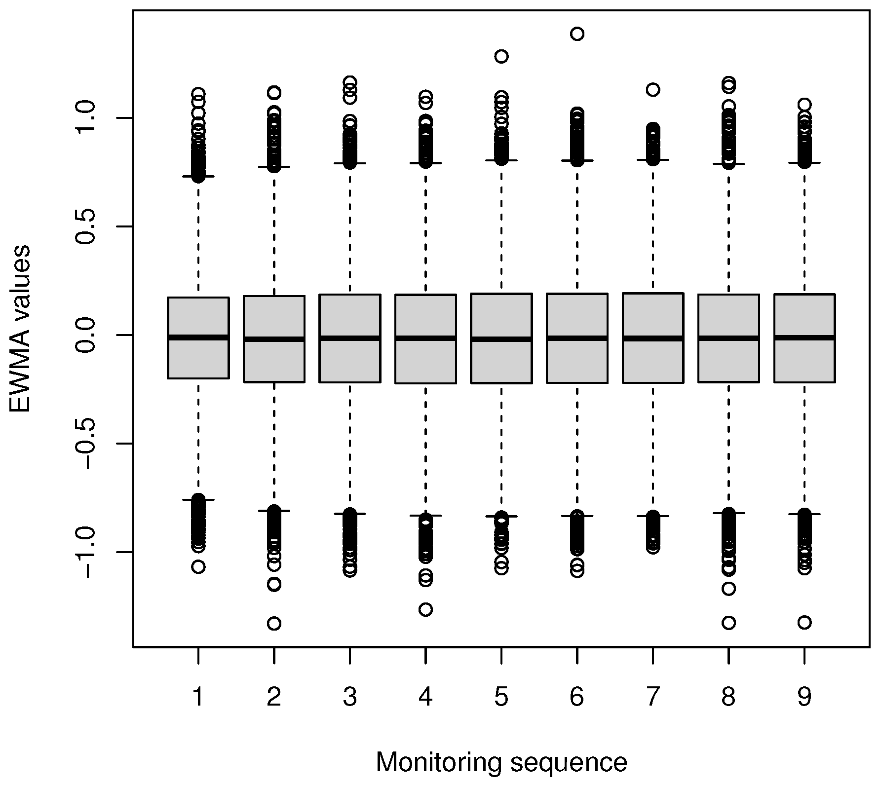
It should be noted that, except for the first two monitoring instances, the estimated conditional marginal distribution of the EWMA statistic remains practically invariant. It could be stated that the distribution of the first two monitoring instances is similar to those obtained for the remaining instances. This can be more clearly seen in Figure 2, which shows the approximate estimated distributions of the first nine monitoring instances.
Table 2 displays the estimated lower and upper control limits of the Phase I EWMA charts in the SREM calculated on five sets of k = 50 independent samples of size n = 5 randomly generated from the standard normal distribution. Each pair of control limits was computed for both the traditional and the probability limit formulations of the EWMA statistic with λ I = 0.6 . The results presented in Table 1 suggest that similar LCL and UCL values are expected for the probability limit approach across each of the k = 50 monitoring instances of the same set of preliminary samples. Table 2 reports the maximum and minimum values observed for each set of 50 samples, which are used as estimates for the lower and upper control limits of the Phase I EWMA chart in the adapted Shen’s formulation for the SREM. The final two columns of the table contain the estimates of the control limits according to Zwetsloot et al. [4]. It is worth mentioning that the control limits calculated for both methodologies are approximately the same for each set of samples. However, the ones calculated for the probability limit approach are always slightly narrower. Although the respective results are not reported, similar conclusions to those presented were obtained for n = 10 and other explored λ I values in combination with the established values of the sample size.
Moreover, the detection abilities for both formulations of the Phase I EWMA chart in the SREM, together with those of the conventional Phase I X ¯ charts (with both the R and the S estimators for the normal process dispersion), were estimated by Formulae (8) and (9) for each proposed out-of-control scenario. The results for the Phase I EWMA charts with λ I = 0.6 and the conventional X ¯ R and X ¯ S schemes are provided in Table 3. All of the control charts under investigation were calibrated to handle sets of k = 50 preliminary samples of the same size n and to reach a nominal FAR level of 1 % .
The simulated results suggest that the ability of each control chart studied to detect true signals improves as the process mean increases. Their ability to detect true signals improves as the size of the samples used for monitoring increases as well. Except for the diffuse shifting pattern, for which all schemes show rather poor detection power, the investigated control charts can detect different types of changes in the process mean. However, the SREM seems to be a more effective option for retrospective monitoring, especially for detecting relatively small increases in the process mean, even when the conventional formulation of the Phase I EWMA control chart is used. The version of the SREM that implements the Phase I EWMA control chart with probability limits exhibits the best detection performance among the examined charts, as its probabilities of correctly signaling are consistently higher in all explored out-of-control scenarios.
It is worth mentioning that Zwetsloot’s Phase I EWMA chart does not outperform the two conventional X ¯ charts when out-of-control samples are scattered or hidden among the in-control ones. Recall that X ¯ is especially designed for detecting localized shifts in the mean. However, the Phase I EWMA chart with probability limits shows rather similar performance to that of its X ¯ counterparts for detecting localized shifts. In addition, even in the diffuse out-of-control scenario, the Phase I EWMA chart with probability limits seems to outperform the other charts investigated.
On the other hand, all of the control charts considered tend to signal wrong alarms more frequently as the process mean and the sample size increase. The results of the simulation study suggest that Phase I EWMA charts are more prone to this issue. This finding is not entirely unexpected, since EWMA charts are sequentially dependent schemes, meaning that a sample signaling an alarm is likely to trigger a subsequent signal. To mitigate an increase in false alarms, it is recommended to inspect the initial set of preliminary samples one by one sequentially, removing the out-of-control samples from the retrospective analysis as soon as they are identified.

5. Simulated Example

To illustrate the performance of the investigated charts, a simulated example involving the localized shift pattern is presented. The localized change in the normal mean was the out-of-control scenario, for which the conducted simulation study suggests less differentiated performance of the proposed charts. A set of k = 50 preliminary random samples of size n = 5 was generated according to the localized shift pattern. As stated in Zwetsloot et al. [4], a model for localized shifts in the normal process mean was established, including all observations in a sample with a 90 % probability of being drawn from the in-control N ( μ 0 , σ 2 ) distribution and a 10 % probability of being drawn from the out-of-control N ( μ 1 , σ 2 ) distribution, where μ 1 = μ 0 + δ σ with δ R + .
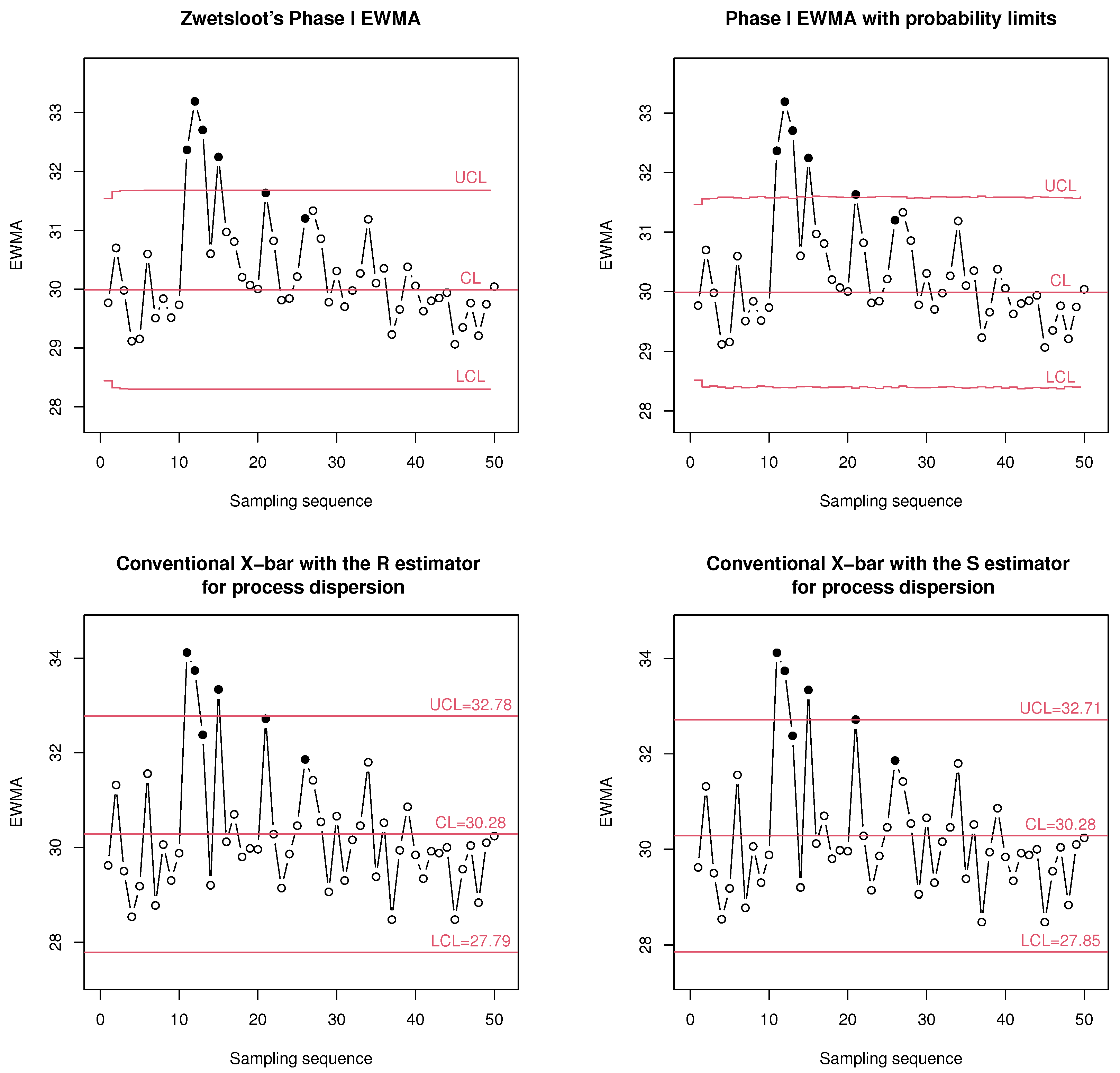
For sample generation, it was assumed that μ 0 = 30 , σ = 2 , and δ = 0.5 so that out-of-control samples undergo a unitary increase in the mean. The implementation of the above-described model for localized changes showed samples 11, 12, 13, 15, 21, and 26 to be out of control. From the randomly generated set of k = 50 samples, it was determined by Equation (5) that the robust estimate for the target normal mean is μ ^ = 29.99 , while the traditional efficient estimate is X ¯ ¯ = 30.28 . It is notable that the estimate obtained by the SREM closely aligns with the actual nominal value of the in-control mean. Additionally, the estimates of the normal standard deviation derived from all of the considered methods were found to be very similar.
Both Zwetsloot’s and the adapted version with probability limits of the Phase I EWMA charts, along with the conventional X ¯ control charts for the simulated example, were drawn. Figure 3 displays the corresponding charts. The generated out-of-control samples are shown as solid black points in all charts. All charts correctly identify samples 11, 12, and 15 as being out of control and fail to detect sample 26. In addition, both conventional X ¯ control charts also fail to identify sample 13, although it is in fact an out-of-control one. The adapted version of the probability limit EWMA chart not only identifies sample 13, but is the only one to correctly detect sample 21. The conventional X ¯ control chart with the S estimator for the normal process dispersion was the only method that nearly detected sample 21, although it ultimately failed to do so. Similarly, not even Zwetsloot’s Phase I EWMA chart successfully identified this sample.
The preceding paragraph reflects the main aspect of the discussion carried out. The results from the conducted simulation study indicate that the conventional methodologies for monitoring the location level, as well as the monitoring method introduced by Zwetsloot et al. [4] for normal processes, tend to overestimate the decision threshold. As a result, these methods may fail to detect samples that are, in fact, out of control. It is also important to note that the investigated scenario involved only a relatively small increase in the process mean.

6. Concluding Remarks and Recommendations

Zwetsloot et al. [4] attempt to extend the application of EWMA charts to Phase I analysis, but the design they propose contains methodological inaccuracies. This paper introduces an alternative approach that improves the detection capability of the Phase I EWMA chart in the SREM. Specifically, the proposed design adapts the dynamic probability limit EWMA chart—originally developed by Shen et al. [6] for Phase II prospective monitoring—for use in Phase I retrospective analysis. Our simulation study demonstrates that the probability limit formulation of the Phase I EWMA chart in the SREM is at least as effective as some existing and conventional Phase I control methodologies when detecting certain types of data anomalies is required.
Although the original design of the EWMA chart for the retrospective monitoring of normal samples is insufficiently accurate, the SREM still makes a significant contribution to the search for and implementation of new methodologies for Phase I analysis. The SREM, as was originally conceived, provides relevant and crucial insights that are steering the development of new and more accurate methodologies for process control in the retrospective stage of monitoring. These insights centrally include robust parameter estimation and the extensive use of EWMA charts in Phase I analysis.
The reconsideration of the SREM presented in this article proposes a more suitable way to estimate the decision threshold of the EWMA chart for Phase I, which conceptually aligns better with the nature of control methodologies based on the FAR. The methodology proposed by Shen et al. [6] plays a pivotal role in this development. The adaptation of the algorithm introduced by Shen in the design of the EWMA chart enhances the analytical accuracy of Phase I assessments of normal processes conducted through the SREM. Consequently, in practical applications within the productive sector, for instance, the proposed methodology represents an effective analytical technique for detecting various types of anomalies present in the data that are due to not-so-substantial changes in the process, even in cases where preliminary samples of different sizes are available and the parameters associated with the formal characterization of the process under consideration are unknown. The most widely used methodology, the X ¯ chart, is only effective in detecting localized outlying samples resulting from significant changes in the process.
The adaptation of the EWMA chart with probability limits for Phase I monitoring facilitates the design of control methodologies that can be applied to virtually any parameter, regardless of the distribution of the variable characterizing process quality. This design could accommodate monitoring schemes involving time-varying sample sizes, as well as individual observations. Moreover, the probability limit approach provides a basis for addressing the correlation structure inherent in retrospective comparisons of charting statistics against fixed control limits, as discussed in Chakraborti et al. [2] and referenced in Section 2. In this context, it is recommended that the resulting FAPr-based control charts be compared with those proposed by Champ and Chou [26] and Champ and Jones [27].
On the other hand, Phase I EWMA schemes can be designed based on the probability limit approach and robust M-scale estimators for the process mean, like those used by Bataineh et al. [28], instead of the robust estimator proposed by Zwetsloot et al. [4]. For further research, it is also possible to compare the performance of the proposal discussed in this article with those developed by Bataineh et al. [28] and/or Sanaullah et al. [29].

Author Contributions

All authors contributed equally to the conceptualization, methodology, software design, and formal analysis of the obtained results of this research work. The preparation of the original draft in English, as well as the writing, review, and editing of the final version of the article, were carried out by C.A.P. The administrative aspects related to the publication were the responsibility of V.H.M. All authors have read and agreed to the published version of the manuscript.

Funding

This research received financial and administrative support from the Universidad de Córdoba, Colombia.

Data Availability Statement

The computer programs needed for this research work were created by the authors in R language and are available upon the request of interested parties to the corresponding author.

Acknowledgments

The authors acknowledge the Universidad de Córdoba, Colombia, for the administrative, technical, and financial support.

Conflicts of Interest

The authors declare no conflicts of interest. No person and/or institution, other than the authors, had any role in the design of the study; in the collection, analysis, or interpretation of the data; in the writing of the manuscript; or in the decision to publish the results.

Abbreviations

The following abbreviations are used in this manuscript:
CUSUMCumulative sum
EWMAExponentially weighted moving average
FAPFalse alarm percentage
FAPrFalse alarm probability
FARFalse alarm rate
SQCStatistical quality control
TAPTrue alarm percentage

References

  1. Jensen, W.A.; Jones-Farmer, L.A.; Champ, C.W.; Woodall, W.H. Effects of parameter estimation on control chart properties: A literature review. J. Qual. Technol. 2006, 38, 349–364. [Google Scholar] [CrossRef]
  2. Chakraborti, S.; Human, S.; Graham, M.A. Phase I statistical process control charts: An overview and some results. Qual. Eng. 2009, 21, 52–62. [Google Scholar] [CrossRef]
  3. Jones-Farmer, L.A.; Woodall, H.W.; Steiner, S.H.; Champ, C.W. An overview of Phase I analysis for process improvement and monitoring. J. Qual. Technol. 2014, 46, 265–280. [Google Scholar] [CrossRef]
  4. Zwetsloot, I.; Schoonhoven, S.; Does, R. A robust estimator for location in Phase I based on an EWMA chart. J. Qual. Technol. 2014, 46, 302–316. [Google Scholar] [CrossRef]
  5. Roberts, S.W. Control chart tests based on geometric moving averages. Technometrics 1959, 42, 239–260. [Google Scholar] [CrossRef]
  6. Shen, X.; Zou, C.; Jiang, W.; Tsung, F. Monitoring Poisson count data with probability control limits when sample sizes are time- varying. Nav. Res. Logist. 2013, 60, 625–636. [Google Scholar] [CrossRef]
  7. Montgomery, D.C. Introduction to Statistical Quality Control, 5th ed.; John Willey & Sons: New York, NY, USA, 2005. [Google Scholar]
  8. Hillier, F.S. X ¯ and R chart control limits based on a small number of subgroups. J. Qual. Technol. 1969, 1, 17–26. [Google Scholar] [CrossRef]
  9. Yang, C.H.; Hillier, F.S. Mean and variance control chart limits based on a small number of subgroups. J. Qual. Technol. 1970, 2, 9–16. [Google Scholar] [CrossRef]
  10. King, E.P. Probability limits for the average chart when process standards are unspecified. Ind. Qual. Control 1954, 10, 62–64. [Google Scholar]
  11. Janacek, G.J.; Meikle, S.E. Control charts based on medians. Statistician 1997, 46, 19–31. [Google Scholar] [CrossRef]
  12. Tatum, L. Robust estimation of the process standard deviation for control charts. Technometrics 1997, 39, 127–141. [Google Scholar] [CrossRef]
  13. Schoonhoven, M.; Riaz, M.; Does, M. Design and analysis of control charts for standard deviation with estimated parameters. J. Qual. Technol. 2011, 43, 307–333. [Google Scholar] [CrossRef]
  14. Rocke, D.M. Robust control charts. Technometrics 1989, 31, 173–184. [Google Scholar] [CrossRef]
  15. Graham, M.A.; Human, S.W.; Chakraborti, S. A Phase I non-parametric Shewhart-type control chart based on the median. J. Appl. Stat. 2010, 37, 1795–1813. [Google Scholar] [CrossRef]
  16. Schoonhoven, M.; Nazir, H.Z.; Riaz, M.; Does, R.J.M.M. Robust location estimators for the X ¯ control chart. J. Qual. Technol. 2011, 43, 363–379. [Google Scholar] [CrossRef]
  17. Schoonhoven, M.; Does, R.J.M.M. A robust standard deviation control chart. Technometrics 2012, 54, 73–82. [Google Scholar] [CrossRef]
  18. Schoonhoven, M.; Does, R.J.M.M. A robust X ¯ control chart. Qual. Reliab. Eng. Int. 2013, 29, 951–970. [Google Scholar] [CrossRef]
  19. Nazir, H.Z.; Riaz, M.; Does, R.J.M.M.; Abbas, N. Robust CUSUM control charting. Qual. Eng. 2013, 25, 311–324. [Google Scholar] [CrossRef]
  20. Vargas, J.A. Robust estimation in multivariate control charts for individual observations. J. Qual. Technol. 2003, 35, 367–376. [Google Scholar] [CrossRef]
  21. Jensen, W.A.; Birch, J.B.; Woodall, W.H. High breakdown estimation for Phase I multivariate control charts. Qual. Reliab. Eng. Int. 2007, 23, 615–629. [Google Scholar] [CrossRef]
  22. Oyeyemi, G.M.; Ipinyomi, R.A. A robust method of estimating covariance matrix in multivariate data analysis. Afr. J. Math. Comput. Sci. Res. 2010, 3, 1–18. [Google Scholar]
  23. Yañez, S.; González, N.; Vargas, J.A. Hotelling’s T2 control charts based on robust estimators. Dyna 2010, 163, 239–247. [Google Scholar]
  24. Ahmadi, M.M.; Shahriari, H. Robust monitoring of simple linear profiles using M-estimators. Comput. Res. Prog. Appl. Sci. Eng. 2022, 8, 1–7. [Google Scholar] [CrossRef]
  25. Neto, E.D.A.L.; Rauber, C.; Borges, H.F.D.N.; Lima-Filho, L.M.A. Process monitoring using robust regression control charts. Qual. Reliab. Eng. Int. 2025. early view. [Google Scholar] [CrossRef]
  26. Champ, C.W.; Chou, S.P. Comparison of standard and individual limits Phase I Shewhart X ¯ , R and S charts. Qual. Reliab. Eng. Int. 2003, 19, 161–170. [Google Scholar] [CrossRef]
  27. Champ, C.W.; Jones, L.A. Designing Phase I charts with small sample sizes. Qual. Reliab. Eng. Int. 2004, 20, 497–510. [Google Scholar] [CrossRef]
  28. Bataineh, A.A.M.F.; Saeed, N.; Obeidat, A.F.S.; Kamal, S.; Abu-Shawiesh, M.O.A. Robust point M-scale estimators for monitoring the mean of EWMA control chart under the normal process. Ain Shams Eng. J. 2022, 13, 101796. [Google Scholar] [CrossRef]
  29. Sanaullah, A.; Chaudhary, A.M.; Hanif, M.; Sharma, P. EWMA control charts based on robust estimators: A powerful tool for monitoring a process with a non-normal distribution. J. Comput. Appl. Math. 2024, 449, 115919. [Google Scholar] [CrossRef]
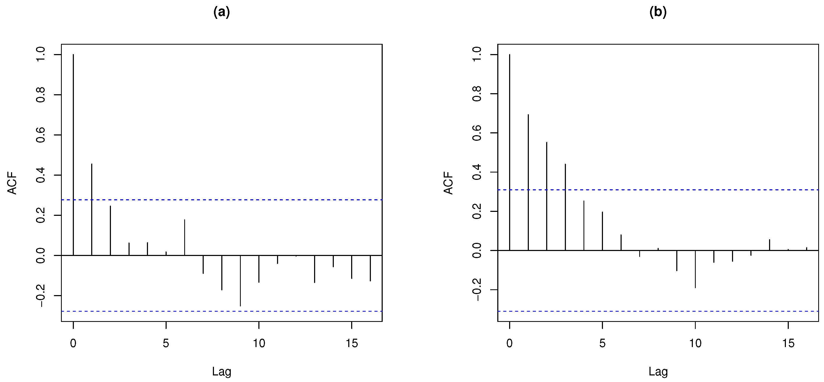
Figure 1. Autocorrelation function of the EWMA statistic with λ I = 0.6 for (a) a simulated set of 50 normal samples of size 5 and (b) the piston rings example.
Processes 13 01381 g001
Figure 2. The approximated marginal distribution of the EWMA statistic with λ I = 0.6 and n = 5 for the first nine monitoring moments.
Processes 13 01381 g002
Figure 3. Phase I EWMA and conventional X ¯ control charts for the simulated example.
Processes 13 01381 g003
Table 1. The approximated in-control conditional marginal distribution of the EWMA statistic with λ I = 0.6 and n = 5 at each monitoring moment t = 1 , , 50 .
Moment Q 0.25 Q 0.50 Q 0.75 MeanSD
1−0.24439−0.057640.13004−0.057750.27729
2−0.25912−0.057040.14350−0.057360.29828
3−0.26074−0.058560.14559−0.057280.30035
4−0.26113−0.057710.14667−0.057470.30091
5−0.26018−0.056940.14625−0.056690.29981
6−0.25975−0.057410.14547−0.057050.30027
50−0.26050−0.057310.14637−0.057880.30056
Table 2. The control limits for both formulations of the Phase I EWMA chart in the SREM with λ I = 0.6 , k = 50 , and n = 5 .
ParameterProbability LimitsZwetsloot’s
Estimators Phase I EWMA Phase I EWMA
μ ^ σ ^ LCL UCL LCL UCL
−0.019351.01798−0.792370.75248−0.797220.75852
0.057290.99620−0.695840.80936−0.703940.81852
0.019541.03771−0.766440.80600−0.773400.81248
0.032171.05359−0.769380.83031−0.772910.83725
0.029980.97172−0.703550.76304−0.712540.77250
Table 3. The approximated performance of the Phase I EWMA charts in the SREM with λ I = 0.6 and the conventional Phase I X ¯ charts designed for k = 50 and F A R = 0.01 .
TAP FAP
δ δ
Approach n 0 . 5 1 . 0 1 . 5 2 . 0 0 . 0 0 . 5 1 . 0 1 . 5 2 . 0
Localized shift pattern
Zwetsloot’s55.426.364.291.3 1.01.11.31.72.5
Phase I EWMA108.352.192.599.8 1.01.21.51.83.5
Shen’s56.128.164.797.4 1.11.21.62.17.1
Phase I EWMA1012.460.895.699.8 1.11.31.72.35.0
Conventional55.828.766.592.3 1.01.01.21.52.0
X ¯ R 1012.360.595.699.9 1.01.11.42.13.1
Conventional55.928.266.592.2 1.01.11.21.51.9
X ¯ S 1012.360.795.299.9 1.01.11.42.13.1
Diffuse shift pattern
Zwetsloot’s51.11.21.52.0 1.01.01.00.80.6
Phase I EWMA101.01.01.11.2 1.01.01.01.01.0
Shen’s51.31.41.82.3 1.01.11.10.90.9
Phase I EWMA101.11.21.31.4 1.11.21.11.01.2
Conventional51.11.21.51.9 1.01.00.90.80.6
X ¯ R 101.01.01.01.0 1.01.00.90.90.8
Conventional51.01.31.51.9 1.01.00.90.70.6
X ¯ S 101.01.01.01.1 1.01.00.90.90.8
Single-step shift pattern
Zwetsloot’s511.456.188.997.7 1.01.11.21.21.2
Phase I EWMA1026.785.898.899.9 1.01.01.21.21.2
Shen’s513.357.089.898.0 1.01.21.41.31.2
Phase I EWMA1026.690.898.899.9 1.01.21.31.31.3
Conventional55.728.367.692.5 1.01.01.21.41.8
X ¯ R 1012.560.495.799.9 1.01.11.31.82.6
Conventional55.828.867.892.7 1.01.01.21.41.8
X ¯ S 1012.360.495.599.9 1.01.01.31.82.6
Multiple-step shift pattern
Zwetsloot’s59.850.186.191.0 1.01.63.85.96.9
Phase I EWMA1023.383.198.199.9 1.02.35.87.48.4
Shen’s511.2552.387.391.8 1.01.63.96.07.1
Phase I EWMA1023.583.898.099.9 1.02.55.47.99.1
Conventional55.225.460.787.9 1.01.32.54.87.2
X ¯ R 1010.854.891.799.4 1.01.64.37.711.0
Conventional55.325.261.388.3 1.01.32.54.77.2
X ¯ S 1011.054.891.899.4 1.01.64.37.710.7
Disclaimer/Publisher’s Note: The statements, opinions and data contained in all publications are solely those of the individual author(s) and contributor(s) and not of MDPI and/or the editor(s). MDPI and/or the editor(s) disclaim responsibility for any injury to people or property resulting from any ideas, methods, instructions or products referred to in the content.