Article

Low-Carbon Optimization Operation of Rural Energy System Considering High-Level Water Tower and Diverse Load Characteristics

School of Electrical Engineering, Xi’an University of Technology, Xi’an 710048, China
*
Author to whom correspondence should be addressed.
Processes 2025, 13(5), 1366; https://doi.org/10.3390/pr13051366
Submission received: 17 February 2025 / Revised: 1 April 2025 / Accepted: 16 April 2025 / Published: 29 April 2025
(This article belongs to the Section Energy Systems)

Abstract

:
Against the backdrop of the steady advancement of the national rural revitalization strategy and the dual-carbon goals, the low-carbon transformation of rural energy systems is of critical importance. This study first proposes a comprehensive architecture for rural energy supply systems, incorporating four key dimensions: investment, system configuration, user demand, and policy support. Leveraging the abundant wind, solar, and biomass resources available in rural areas, a low-carbon optimization model for rural energy system operation is developed. The model accounts for diverse load characteristics and the integration of elevated water towers, which serve both energy storage and agricultural functions. The optimization framework targets the multi-energy demands of rural production and daily life—including electricity, heating, cooling, and gas—and incorporates the stochastic nature of wind and solar generation. To address renewable energy uncertainty, the Fisher optimal segmentation method is employed to extract representative scenarios. A representative rural region in China is used as the case study, and the system’s performance is evaluated across multiple scenarios using the Gurobi solver. The objective functions include maximizing clean energy benefits and minimizing carbon emissions. Within the system, flexible resources participate in demand response based on their specific response characteristics, thereby enhancing the overall decarbonization level. The energy storage aggregator improves renewable energy utilization and gains economic returns by charging and discharging surplus wind and solar power. The elevated water tower contributes to renewable energy absorption by storing and releasing water, while also supporting irrigation via a drip system. The simulation results demonstrate that the proposed clean energy system and its associated operational strategy significantly enhance the low-carbon performance of rural energy consumption while improving the economic efficiency of the energy system.

1. Introduction

In the context of the ongoing global energy transition and the steady advancement of China’s rural revitalization strategy [1], the low-carbon optimization of rural energy systems holds substantial theoretical and practical significance. Currently, energy consumption in rural households primarily encompasses heating, cooling, cooking, lighting, and the operation of other household appliances. This consumption pattern is characterized by a high degree of carbon intensity and a reliance on non-clean energy sources. The three dominant fuels are coal (33.8%), straw (27.8%), and firewood (15.7%), while the adoption of renewable energy sources such as solar energy (2.4%) and biogas (2.6%) remains limited [2]. Rural energy-related activities account for approximately 60% of the nation’s total CO2 emissions. Furthermore, rural regions often face challenges such as unreliable energy supply and environmental degradation [3]. In light of the “dual-carbon” targets—peaking carbon emissions and achieving carbon neutrality—the ecological sustainability and low-carbon development of rural energy supply systems are of strategic importance. Rural areas typically possess abundant renewable resources, including wind, solar, and biogas, and offer significant potential for the deployment of distributed energy systems [4]. Simultaneously, the emergence and expansion of agricultural industrial parks have led to an increase in energy demand, which is becoming increasingly diverse in nature. Against this backdrop, there is an urgent need to construct clean energy systems capable of accommodating varied load types, enabling coordinated multi-energy coupling, and promoting the localized utilization of renewable resources. Such systems are essential to advancing the low-carbon transition of rural energy infrastructures [5,6]. Recent studies [7,8] have integrated various rural energy types to achieve electrification through energy complementarity, thereby maximizing carbon emission reductions. Other works [9,10] have analyzed the current energy structure in rural regions and proposed targeted strategies to optimize energy usage patterns, contributing to a substantial reduction in the carbon footprint of rural energy consumption.
Electricity demand in rural areas is characterized by high spatial dispersion, strong seasonality, and intermittent usage patterns. Compared with urban loads, rural energy loads generally exhibit weaker responsiveness and lower flexibility. Although rural regions are endowed with abundant wind and solar resources, the uncertainty inherent in their output poses significant challenges to energy system stability and reliability [11,12]. High-rise water towers, commonly deployed in rural settings—particularly in low-lying or infrastructure-deficient areas—serve as gravity-based water storage and supply systems [13]. These towers store water at elevated heights and deliver it to surrounding users using gravitational potential energy. Their structural components typically include the tower body, storage tank, piping system, and support framework [14,15]. Under the growing emphasis on rural clean energy development, the intermittency and variability of wind and solar generation not only result in substantial curtailment but also jeopardize grid stability. High-rise water towers offer a potential solution by storing surplus electrical energy as gravitational potential energy through water pumping, thereby functioning as a form of energy storage. This mechanism can help to flatten load curves by mitigating peak–valley fluctuations. Given these advantages, integrating high-rise water towers into rural clean energy systems presents a promising opportunity. During periods of excess wind and solar generation, water can be pumped and stored; during peak irrigation demand, the stored water can be released to meet agricultural needs. This approach enhances the utilization of renewable resources while buffering against output uncertainty. For instance, ref. [16] explored the use of hybrid energy systems to support rural irrigation in Saudi Arabia, demonstrating superior economic and transmission performance over standalone solar solutions. Ref. [17] developed an optimized operational model for rural clean energy systems from multiple perspectives—including infrastructure, system dynamics, user behavior, and policy—but did not specifically address irrigation load requirements. Ref. [18] proposed a two-layer rural integrated energy scheduling model for biogas-based hydrogen production, effectively reducing wind curtailment and mitigating renewable generation uncertainty. Ref. [19] presented a two-stage decision-making and planning optimization framework for multi-regional rural hybrid renewable energy systems (RHRESs), integrating photovoltaics, wind power, and biogas pools, thereby significantly improving renewable resource utilization. However, none of these studies have considered the application of high-rise water towers—ubiquitous in rural environments—as a dual-purpose solution to address both irrigation demands and the intermittency of wind and solar power output.
With the continuous development of the rural economy, the types of rural energy loads are becoming increasingly diversified, encompassing cold storage facilities, agricultural product processing plants, constant-temperature greenhouses, and other applications with rising energy demands. According to their response characteristics, flexible loads in rural areas can be categorized into shiftable, curtailable, and dispatchable loads. To effectively reduce peak–valley load differences and electricity costs, it is essential to develop targeted demand response strategies tailored to each load type’s flexibility characteristics, thereby enhancing both the economic efficiency and operational stability of rural energy systems. Ref. [20] incorporates rural load profiles and environmental factors into rural microgrid design, improving photovoltaic utilization and economic performance. Ref. [21] proposes a novel rural microgrid architecture by aggregating distributed energy resources and flexible loads. Ref. [22] introduces a dual-response mechanism that coordinates supply and demand in rural settings. Ref. [23] constructs a comprehensive demand response model based on both pricing and incentives, proposing a tiered subsidy mechanism. Ref. [24] adopts an interval optimization model to address the uncertainties in hydrogen-based integrated energy systems during day-ahead scheduling, while incorporating price-based and incentive-based demand response mechanisms in the intraday stage to handle renewable generation and load uncertainty. Ref. [25] integrates a comprehensive demand response scheme into traditional energy systems, promoting the coordination of heterogeneous energy sources and enhancing conversion efficiency. Ref. [26] develops a probabilistic interval model to reflect the stochastic behavior of user demand response, enabling more accurate system-level quantification and adjustment. While some of these works address the uncertainty and methodologies of load response, few consider the intrinsic response characteristics of specific loads. For example, ref. [27] classifies LED equipment in agricultural orchards as shiftable loads and enables their participation in optimal scheduling, yet does not account for irrigation loads in developing viable response plans. Although the above literature provides detailed demand response mechanisms, traditional approaches often treat all electrical loads homogenously, ignoring their internal structure. However, certain electrical loads require uninterrupted operation over specific timeframes, or a constant total energy usage throughout the scheduling horizon. Thus, demand response plans developed without detailed load classification lack practicality and feasibility. Only by implementing both price-based and incentive-based demand response strategies that are grounded in a fine-grained understanding of each flexible load’s operational constraints can economically viable and technically feasible response plans be achieved. In parallel with advances in energy optimization and low-carbon rural strategies, substantial progress has also been made in rural energy storage technologies. Ref. [28] addresses power outages in rural areas by integrating supercapacitors as backup power sources for agricultural applications, utilizing their superior energy storage and rapid discharge characteristics. Ref. [29] designs a remote monitoring system for rural energy storage based on NB-IoT wireless communication technology, which enhances maintenance efficiency and supports the stable operation of storage infrastructure. Moreover, under the broader framework of rural revitalization, the importance of agricultural mechanization is increasingly emphasized. Ref. [30] analyzes agricultural mechanization in Heze City, offering practical recommendations based on statistical analysis and policy interpretation. Ref. [31] further identifies agricultural mechanization as a key indicator of rural modernization, evaluates its developmental constraints, and proposes strategies to promote its coordinated integration with rural economic growth.
The reviewed literature demonstrates that although rural areas possess abundant wind, solar, and biomass resources, their energy structures remain underdeveloped, with low levels of clean energy utilization. Existing research on the optimal operation of rural energy supply systems often overlooks the potential of utilizing high-rise water towers (HWTs) for dual purposes—storing water to meet irrigation demands while simultaneously mitigating the uncertainty of intermittent renewable energy sources, thus enhancing the low-carbon performance and clean energy regulation capacity of rural energy systems. Moreover, most current studies on demand-side response tend to generalize energy consumption as a homogeneous electrical load, failing to account for the diverse nature of rural energy demands by classifying and modeling distinct load types. To address these gaps, this paper proposes a comprehensive rural clean energy system (CES) that integrates high-rise water towers and accommodates the diverse characteristics of rural energy loads, including cooling, heating, electricity, and gas demands within rural residential and production areas. When wind and solar resources are plentiful, water is pumped into the towers for storage and later discharged during peak irrigation periods, thereby improving renewable energy utilization and mitigating the adverse effects of output uncertainty. Simultaneously, this study incorporates detailed load typologies and develops tailored, practical response strategies based on the specific responsiveness of each load type, effectively reducing peak–valley disparities and enhancing the overall economic performance of the energy system.
The main contributions of this study are summarized as follows.
Job Description
(1)  This study develops a comprehensive model of the internal components of the clean energy system (CES), accounting for the uncertainty associated with wind and solar power generation. It further classifies the diverse energy loads present in rural areas and formulates a practical demand response strategy tailored to the specific response characteristics of each load type. Notably, the unique irrigation load in rural settings is addressed through the integration of high-rise water towers with drip irrigation systems, enabling both efficient water resource management and enhanced utilization of intermittent renewable energy sources.
(2)  Considering the load balance constraints of cooling, heating, electricity, gas, and irrigation, this paper establishes a multi-objective optimization operation model for the rural clean energy system (CES), aiming to maximize economic benefits while achieving the highest level of low carbonization. The model fully leverages rural high-rise water towers for water storage, effectively satisfying irrigation demands while mitigating the uncertainty of wind and solar power output. Through the coordinated optimization of wind, solar, and biomass resources, the system enhances both energy utilization efficiency and operational stability in rural areas.
(3)  Based on annual load data from rural areas, an ordered clustering analysis and typical scenario extraction are conducted to represent the variability of energy demand and renewable generation. The clean energy system (CES) is subsequently simulated using these representative typical days. The simulation results demonstrate that the proposed CES operational strategy exhibits superior economic performance and enhanced low-carbon outcomes under a comparative analysis of multiple scenarios.
The remainder of this paper is organized as follows: Section 1 presents an introduction and outlines the structure of the rural clean energy system. Section 2 describes the optimization operation model of the clean energy system (CES). Section 3 focuses on the extraction of typical scenario days, considering the diversity of rural loads. Section 4 evaluates the effectiveness of the proposed method through simulation examples. Finally, Section 5 concludes the paper.

2. Rural Clean Energy System Structure

2.1. System Introduction

The rural energy supply system proposed in this paper integrates energy suppliers, energy storage aggregators, and various production and residential loads. It is structured around a clean energy system and electric energy storage, each invested in and developed by the respective energy suppliers and storage aggregators. The clean energy system serves as the conduit for electricity transmission, supplying power to diverse energy loads. Simultaneously, it incorporates policy-driven pricing mechanisms and incentive-based demand response strategies to optimize load management, ensuring the clean energy system operates in an efficient, balanced, and cost-effective manner. The specific system architecture is illustrated in Figure 1.
The energy storage system purchases the excess energy that the clean energy system (CES) has not absorbed at a low price. When the CES is unable to meet the load demand, the energy storage system sells stored energy at the standard energy supply price of the CES, thereby generating profits. Energy suppliers implement demand response policies tailored to the characteristics of various rural loads. Industrial parks, characterized by large loads and significant peak-to-valley differences, are highly sensitive to their own operational costs as well as fluctuations in electricity prices. Consequently, both incentive-based and price-based demand response strategies can be employed to facilitate energy transfer. In contrast, agricultural energy demand, primarily driven by irrigation needs, exhibits strong seasonality and is both interruptible and shiftable. Price subsidies can be used to facilitate energy transfer, making incentive-based demand response particularly applicable in this context.

2.2. Clean Energy System Structure

The internal structure of the rural clean energy system is illustrated in Figure 2. Energy suppliers invest in clean energy generators and power conversion units, working in tandem to meet the energy demands of rural life and production. The clean energy supply is derived from solar, wind, and biomass sources. Each generator is designed to supply energy for cooling, heating, and electricity needs, while the gas load is directly provided by the biogas tank. CES loads are categorized into two main types: residential loads and production loads within industrial parks. Residential loads primarily cover the daily energy needs of villagers, including lighting, heating, cooking, and other essential services. Production energy demands are divided into four categories: constant temperature greenhouses, cold storage facilities, agricultural product processing plants, and agricultural irrigation. The specific cooling, heating, and electricity energy demands for each type of load are detailed in Figure 2. In cases where the CES is unable to meet the load demand, electricity is purchased from the power grid.

2.3. Demand Response Model

2.3.1. Price-Based Demand Response Model

The price-based demand response discussed in this paper involves dividing the entire time period into three stages—normal, peak, and valley—based on the load demand across the 24 dispatch periods. Energy suppliers adjust electricity prices according to the varying energy consumption periods and load demands to encourage users to shift their energy consumption, thereby achieving peak shaving and valley filling. Price-based demand response is relatively straightforward and easy to implement in practice, making it an effective strategy for managing energy demand.
Q e 1 Q e 2   Q e t = Q e 1 0 0 0 Q e 2 0 0 0 0 Q e t   ·   e 11 e 12 e 1 t e 21 e 22 e 2 t e t 1 e t 2 e t t   ·   Δ p e 1 / p e 1 Δ p e 2 / p e 2 Δ p e t / p e t + Q e 1 Q e 2   Q e t
wherein Q e 1 and Q e 1 are the loads before and after the implementation of time-of-use electricity prices; e t 1   e t 2 e t t is the elasticity coefficient of the electricity load; p e t and Δ p e t are the electricity price and electricity price change during period t.

2.3.2. Incentive Demand Response Model

Based on the principles of the incentive-based demand response mechanism, it can be categorized into two types: direct load response and interruptible load response. This paper focuses on the direct load response, where energy consumption is directly adjusted in response to demand, following the signing of a compensation agreement between the user and the energy supplier. In this arrangement, the user receives corresponding economic compensation, thereby facilitating energy transfer [32].
C I D R = P t I D R Δ Q e t P t I D R = P 1 , t I D R , Q min Δ Q e t Q 1 P 2 , t I D R , Q 1 < Δ Q e t Q 2   P n , t I D R , Q max < Δ Q e t
where C I D R is the cost of implementing an incentive demand response for CES; P t I D R is the unit economic compensation cost of the incentive response in period t; Δ Q e t is the load response at time t; Q 1 and Q 2 are the segment critical points; Q min and Q max are the minimum and maximum segment critical points.

2.3.3. Participation Mode of Demand Response

In summary, when responding to the system demand side, the various types of loads in the clean energy system have different response modes and participation modes according to their own different characteristics [33]. The specific situation is shown in Table 1.

2.4. Low-Carbonization Evaluation Model

The clean energy system (CES) discussed in this paper requires an evaluation of its low-carbonization level. CES energy is primarily categorized into clean energy and carbon-emitting energy sources. To enable consistent evaluation, the standard coal conversion factor is applied to convert various energy types into a common unit, allowing for the quantification of the clean energy proportion in the CES energy supply over a 24-h period. This process facilitates the visualization of the low-carbon level throughout the energy supply period. The model is represented by Formula (3).
n = 1 N G n X n i = 1 I E i γ i 0 n = 1 N G n X n i = 1 I E i γ i 0
In the formula, G n is the load capacity met by the ith clean energy; X n is the standard coal conversion coefficient per kilowatt-hour of electricity of the ith clean energy; E i is the load capacity met by the ith carbon emission energy; γ i is the standard coal conversion coefficient per kilowatt-hour of electricity of the ith carbon emission energy.

2.5. Energy Storage System Model

The energy storage system in this paper operates independently of the clean energy system. The energy storage aggregator purchases excess energy from the CES at a price lower than the standard energy supply price and subsequently sells it back to the CES at the normal energy supply price to fulfill the remaining load demand. The corresponding model constraints are represented by Formula (4):
E E S S , t = E E S S , t 1 ( 1 e l o s s ) + [ η a b s P a b s , t ( 1 / η r e l ) P r e l , t ] Δ t 0 P a b s , t ε a b s , t P t max 0 P r e l , t ε r e l , t P t max 0.1 E E S S max E E S S , t 0.9 E E S S max ε r e l , t + ε a b s , t 1
In the formula, E E S S , t is the storage capacity of the energy storage device at time t, kW·h; e l o s s is the energy loss rate at time t; η a b s , η r e l is the charge and discharge efficiency; Δ t is the charge and discharge time interval; ε a b s , t , ε r e l , t is the charge and discharge state at time t, which is a 0–1 state variable; P t max is the maximum charge and discharge power, kW; E E S S max is the maximum capacity of the energy storage device, kW·h.

2.6. High-Level Water Tower Pump Model

The high-level water tower is a key water supply facility currently in use. It has the capacity to store a significant amount of water, which is then provided to meet the needs of surrounding residents for both domestic and agricultural purposes. The water supply capacity of a high-level water tower is influenced by its construction height and storage capacity. Its primary function is to store and regulate local water resources. Typically constructed from reinforced concrete, the high-level water tower is designed for high structural stability and load-bearing capacity. It is often used in conjunction with a ground pressure distribution pump station to maintain stable water pressure during operation, especially when combined with a regulator and other related equipment. High-level water towers are usually built at elevated sites, which enhances the water supply pressure and contributes to the stability of the water distribution system. The height of a high-level water tower is generally determined by factors such as terrain, altitude, and local planning guidelines, typically ranging from 30 m to 100 m. The tower’s capacity is largely based on the local demand. In this study, the high-level water tower is situated in a rural area, where its primary role is to support agricultural irrigation while also absorbing excess rural clean energy. The relevant model constraints for the high-level water tower, equipped with a centrifugal water pump, are given by Equations (5)–(12):
γ = ρ g Q G = γ Q
wherein γ is the density of the liquid, N/m3; Q G is the weight flow rate, N/s; Q is the volume flow rate, m3/s.
H = E 2 E 1
where H is the head of the pump; E 2 is the energy per unit weight of liquid at the pump outlet, m; E 1 is the energy per unit weight of liquid at the pump inlet, m.
E 1 = p 1 γ + v 1 2 2 g + z 1 E 2 = p 2 γ + v 2 2 2 g + z 2
In the formula, p 2 , p 1 are the pressures of the liquid at the pump outlet and inlet, N; v 2 , v 1 are the absolute velocities of the liquid at the pump outlet and inlet, m/s; z 2 , z 1 are the distances from the pump outlet and inlet to the measurement reference plane, m.
The pump head can be written as follows:
H = p 2 p 1 γ + v 2 2 v 1 2 2 g + ( z 2 z 1 )
The power of a pump usually refers to the input power, the power transmitted from the prime mover to the pump shaft, which is generally called shaft power.
N e = γ Q H η = N e N
where N is the input power and shaft power of the pump, kW; N e is the effective energy obtained from the pump for the liquid delivered by the pump per unit time, kW.
Q c h = N / ( 9.81 H η c h )
where Q c h is the water flow rate of the pump, m3/s; η c h is the working efficiency of the pump.
V t + 1 = V t ( 1 r l o s s ) + 3600 U c h t Q c h t U r e l t ( 1 / η f ) Q r e l t
In the formula, V t + 1 and V t are t + 1 the water storage capacity of the water tower at time and time, t m3; r l o s s is the loss rate of the water tower reservoir; U c h t and U r e l t are the state variables of pumping and drainage of the water pump unit, respectively; η f is the drainage efficiency of the water tower; Q r e l t is the drainage flow rate of the water tower at time and time, t m3/s.
0 V t V max Q min c h Q t c h Q max c h Q min r e l Q t r e l Q max r e l
In the formula, V max is the capacity of the water tower; Q max c h and Q min c h are the maximum and minimum pumping rates of the water tower pump, m3/s; Q max r e l and Q min r e l are the maximum and minimum water discharge rates of the water tower pump, m3/s; Q t c h and Q t r e l are the pumping and discharge rates of the water tower pump at each moment, t m3/s.

3. Rural CES Optimization Operation Model

3.1. Objective Function

While the CES new energy output meets the load, it may also need to purchase electricity from energy storage aggregators and rural power grids to meet the remaining load. In the energy supply process, the objective functions of the CES are to maximize economic benefits and maximize the degree of low-carbon energy supply.
max F 1 = g G t T R i n , t g j = 1 J t = 1 T C O M , t j j = 1 J C D E j C D R j = 1 J C R M , t j t = 1 T C e , t t T C b u y , t
max F 2 = n = 1 N G n X n i = 1 I E i γ
In the formula, F 1 is the overall economic benefit of the CES; R i n , t g is the benefit of the CES when it meets the first g type of load at time t ; C O M , t j is the operation and maintenance cost of the unit j at time t ; C D E j is the investment cost of the unit j ; C D R is the demand response cost of the entire scheduling period; C R M , t j is the raw material cost of the unit j at time t ; C e , t is the cost of purchasing electricity from the rural distribution network at time t ; C b u y , t is the cost of the CES purchasing electricity from energy storage aggregators at time t ; F 2 is the low-carbon degree of the CES.
R in , t g = p i n , t g P i n , t g C O M , t j = p o m j P t j C D E j = C ii j r C ii j 365 N C R M , t j = p r m , t j M t j
wherein P i n , t g is the Class g load satisfied by the CES at moment t ; p i n , t g is the energy supply price of the CES for Class g load at moment t ; P t j is the output of the unit at moment t ; p o m j is the operation and maintenance cost of unit j ; C ii j is the initial investment cost of unit j ; r is the residual value coefficient; N is the overall service life; p r m , t j is the unit raw material cost of unit j at moment t ; M t j is the raw material demand of unit j at moment t .

3.2. Constraints

3.2.1. Supply and Demand Balance Constraints

(1) Electric load supply and demand balance constraints.
Since the output of wind and solar power units has a certain degree of uncertainty, in order to ensure the stability of the CES, this paper establishes a wind and solar power output uncertainty set model based on a robust model:
P w p p e , t * = P w p p e , t + η t e w p p e , t P w p p e , t ( η t [ 1 , 1 ] )
P p v e , t * = P p v e , t + γ t e p v e , t P p v e , t ( γ t [ 1 , 1 ] )
wherein P w p p e , t * is the electric load satisfied by wind power at moment t after considering the uncertainty of wind power output; P p v e , t * is the electric load satisfied by photovoltaic at moment t after considering the uncertainty of photovoltaic output; P w p p e , t is the electric load satisfied by wind power at moment t ; P p v e , t is the electric load satisfied by photovoltaic output at moment t ; e w p p e , t , e p v e , t are the error coefficients of wind power and photovoltaic output, respectively.
P w p p e , t + Γ w p p e e w p p e , t P w p p e , t P p v e , t + Γ p v e p v e , t P p v e , t ( P b c e , t + P u e o , t + P r e l , t ) ( Q e t + Δ Q e t + P a b s , t )
wherein Γ w p p e , Γ p v are the robustness coefficients of wind power and photovoltaic power to ensure the controllability of wind power and photovoltaic power supply; Q e t is the amount of life and production electricity load that the CES meets at moment t ; Δ Q e t is the demand response amount of life and production electricity load of the CES at moment t ; P a b s , t , P r e l , t are the charging and discharging power of the energy storage power station at moment t ; P b c e , t is the amount of electricity load that the biogas generator meets at moment t ; P u e o , t is the amount of electricity purchased from the power grid by the CES to meet the electricity load at moment t .
(2) Heat load supply and demand balance constraints.
P u v h , t + P w p p h , t + P b c h , t + P u h o , t = Q h t + Δ Q h t
wherein P u v h , t is the heat load satisfied by the photovoltaic unit at moment t ; P w p p h , t is the heat load satisfied by the wind turbine unit at moment t ; P b c h , t is the heat load satisfied by the biogas unit at moment; P u h o , t is the amount of electricity purchased from the grid by the CES to meet the heat load at moment t ; Q h t is the production heat load satisfied by the CES at moment t ; Δ Q h t is the demand response amount of the CES to meet the production heat load at moment t .
(3) Cooling load supply and demand balance constraints.
P u v c , t + P w p p c , t + P b c c , t + P u c o , t = Q c t + Δ Q c t
In the formula, P u v c , t is the cooling load satisfied by the photovoltaic unit at moment t ; P w p p c , t is the cooling load satisfied by the wind turbine unit at moment t ; P b c c , t is the cooling load satisfied by the biogas unit at moment t ; P u c o , t is the amount of electricity purchased from the power grid by the CES to meet the cooling load at moment t ; Q c t is the production cooling load satisfied by the CES at moment t ; Δ Q c t is the demand response amount of the CES to meet the production cooling load at moment t .
(4) Constraints on gas load supply and demand balance.
Q b c , t = Q gt
where Q b c , t is the biogas supply of the biogas digester at moment t ; Q gt is the CES life gas load at moment t .

3.2.2. Unit Output Constraints

(1) Rural biogas unit output.
P b c e , t + P b c c , t / K c + P b c h , t / K h = V b i o , t η b V b i o = i = 1 I R i C i η c
In the formula, V b i o , t is the amount of biogas used for power generation at each moment t ; η b is the biogas power generation efficiency; K c , K h are the COP values of the electric refrigeration unit and the electric heating unit, respectively; V b i o is the total amount of biogas; R i is the yield of the i th type of crops; C i is the grass-to-grain ratio of the i th type of crops; η c is the average gas production of crops.
V b i o min V b i o V b i o max
V b i o , t min V b i o , t V b i o , t max
In Formulas (23) and (24), V b i o max , V b i o min are the upper and lower limits of the biogas digester capacity, respectively; V b i o , t max , V b i o , t min are the upper and lower limits of the amount of biogas used for power generation at any time t , respectively.
(2) Energy supply units
Wind turbine unit constraints.
0 P w p p e , t + P w p p c , t / K c + P w p p h , t / K h P w p p , t max
where P w p p , t max is the upper limit of wind turbine output at moment t .
PV unit constraints.
0 P p v e , t + P u v c , t / K c + P u v h , t / K h P p v , t max
where P p v , t max is the upper limit of the photovoltaic unit output at moment t .
Energy conversion unit constraints.
0 P E R C , t P E R C , t max
0 P E R H , t P E R H , t max
In Formulas (27) and (28), P E R C , t , P E R H , t are the conversion power of the electric refrigerator and electric boiler at time t , respectively; P E R C , t max , P E R H , t max are the upper limits of the conversion power of the electric refrigerator and electric boiler at time t , respectively.
This paper assumes that the electricity purchased by the CES from the rural power grid is supplied by thermal power units, and the up and down ramp and start and stop constraints of thermal power units are as follows:
P G i , t P G i , t 1 P i , u p P G i , t 1 P G i , t P i , d o w n
In the formula, P G i , t , P G i , t 1 represent the output of the i th thermal power unit at time t , t 1 , respectively; P i , u p , P i , d o w n represent the maximum rising rate and minimum falling rate of the i th thermal power unit, respectively.
( T i , t 1 u p T i , min u p ) ( u i , t 1 u i , t ) 0
( T i , t 1 d o w n T i , min d o w n ) ( u i , t u i , t 1 ) 0
In Formulas (30) and (31), T i , t 1 u p represents the time that the ith thermal power unit has been continuously turned on in the t 1 period; T i , t 1 d o w n represents the time that the i th thermal power unit has been continuously turned off in the t 1 period; u i , t represents the start-stop status of the unit, a 0_1 variable; T i , min u p represents the minimum continuous start-up time of the i th thermal power unit; T i , min d o w n represents the minimum continuous shutdown time of the i th thermal power unit.

3.2.3. Demand Response Constraints

(1) Load change constraint
Δ Q g , t min Δ Q g , t Δ Q g , t max
wherein Δ Q g , t max , Δ Q g , t min are the upper and lower limits of the demand response for the g th load at time t ; Δ Q g , t is the demand response amount for the g th load at time t .

3.2.4. Grid Stability Constraints

(1) Node voltage limits:
V min V i V max , i N
where V i is the voltage amplitude of the node i ; V min , V max is the allowable voltage range (usually ±5% of the rated voltage).
(2) Reactive power balance:
Q gen , i Q load , i Q cap , i = j N B i j V i V j sin θ i θ j
where Q gen , i is the reactive output of the generator; Q load , i is the reactive demand of the load; Q cap , i is the reactive power provided by the reactive compensation device; B i j is the element of the admittance matrix between nodes i , j ; θ i , θ j is the node voltage phase angle.
(3) Frequency stability constraint:
System frequency range:
f min f f max
where f is the real-time frequency of the system; f min , f max is the specified frequency range (for example, 49.5–50.5 Hz).
(4) Stability margin constraint:
Transient stability constraint (rotational kinetic energy equation):
J d ω d t = T m T e
where J is the rotor inertia; ω is the unit angular velocity; T m , T e are the mechanical input and electromagnetic output torques, respectively.
Voltage stability margin:
Q V > 0
This constraint is used to determine whether the system has a risk of voltage collapse.

3.3. CES Optimization Operation Strategy

This paper develops a clean energy system (CES) model tailored to the unique resource endowments and geographical characteristics of rural areas. The CES is designed to meet the comprehensive energy demands—including heating, cooling, and electricity—of both residential and production activities in rural settings. It incorporates the inherent uncertainties associated with wind and solar power generation as well as load fluctuations. Distinct response strategies are formulated according to the response characteristics of different load types. During each scheduling period, the CES conducts an energy optimization process that dynamically allocates and schedules energy resources to balance supply and demand, minimize costs, and maximize system stability and low-carbon performance.
StepOperation Strategy
(1)  The annual data on cooling, heating, and electricity loads in rural areas are collected through field investigations, capturing the temporal variation in energy demand over the course of the year. These data provide a foundational basis for subsequent analysis and model development. The energy consumption patterns and corresponding load curves in rural areas exhibit pronounced seasonal and temporal characteristics, reflecting fluctuations driven by climatic conditions, agricultural activities, and daily living habits.
(2)  Two typical scenarios are extracted using the Fisher optimal segmentation method to simplify and classify the annual load data. This statistical approach partitions the data into representative segments by minimizing intra-group variance and maximizing inter-group variance, thereby enhancing the interpretability and efficiency of subsequent modeling. In this study, two typical scenarios are selected to reflect the characteristic patterns of rural energy demand, facilitating the construction and validation of the CES optimization model under different operating conditions.
(3)  Based on the typical scenarios, error coefficients and robustness coefficients are defined for wind and photovoltaic (PV) outputs to quantitatively reflect the inherent uncertainty associated with wind and solar energy generation. Due to the significant fluctuations in output caused by meteorological variability, incorporating these uncertainty parameters enables the model to better capture real-world dynamics. This enhances the adaptability and resilience of the CES, ensuring stable and reliable system operation under varying external conditions.
(4)  The optimization model of the rural clean energy system (CES) is established through Formulas (1)–(32), integrating the outputs of wind power, photovoltaic generation, grid electricity, and energy storage systems into a unified, multi-energy optimization framework. This comprehensive model simultaneously addresses the coordination of various energy forms—electricity, heat, cooling, gas, and irrigation—while accounting for the operational characteristics and uncertainties inherent in renewable energy sources. By optimizing energy flow and system scheduling, the model effectively balances energy supply and demand, enhances system flexibility, and achieves dual objectives of maximizing economic performance and minimizing carbon emissions, thereby promoting sustainable and efficient rural energy development.
(5)  During the dynamic operation of the model, various load demands and wind power outputs fluctuate across different time periods. To address these variations, the model incorporates the participation of flexible resources in demand response. These flexible resources—such as adjustable production equipment, irrigation systems, and energy storage—can reduce or shift their loads based on real-time system conditions. By strategically balancing supply and demand through load adjustment, the system minimizes reliance on external grid power, reduces peak load pressures, and enhances operational efficiency. This demand response strategy significantly contributes to improving the overall economy of the rural CES while supporting stable and sustainable energy utilization.
(6)  According to Formulas (18) to (21), the model ensures that the CES maintains energy balance across cooling, heating, and electricity loads. Unlike traditional models that focus solely on electric load, this model comprehensively integrates the demand for cooling and heating, enabling the system to simultaneously meet multiple types of energy needs. By coordinating cooling, heating, and electric energy flows, the CES achieves a more holistic and efficient allocation of resources, improving system performance, energy utilization efficiency, and user satisfaction. This multi-energy coordination is crucial for supporting the diversified and seasonal energy demands characteristic of rural life and production scenarios.
(7)  The optimization objectives of the model are twofold: firstly, to maximize the economic benefits of the rural clean energy system (CES), and secondly, to maximize the degree of low carbonization. This dual-objective approach ensures that while the system achieves optimal economic performance—such as reducing energy costs, improving resource utilization, and generating revenue through demand response and energy storage operations—it simultaneously minimizes carbon emissions. By integrating clean energy sources like solar, wind, and biomass, and adopting flexible load management and energy storage strategies, the CES promotes a sustainable and low-carbon energy transformation in rural areas, aligning with national dual-carbon goals and rural revitalization efforts.
(8)  Finally, the optimal dispatching scheme is formed through multi-scenario and multi-period optimization. This approach comprehensively considers the variations in load demand and energy supply across different time periods and scenarios throughout the year. By integrating these dynamic factors into the dispatching strategy, the model ensures that the CES can maintain efficient and stable operation under various conditions. This strategy significantly enhances the system’s flexibility and adaptability, allowing it to effectively respond to fluctuations in load and renewable energy output. Consequently, the multi-scenario and multi-period optimization not only improves the overall operational economy of the CES but also strengthens its robustness and resilience, supporting the goal of achieving low-carbon and sustainable rural energy development.
From the above, it can be seen that the CES constructed in this paper makes full use of the unique wind and solar resources available in rural areas. It takes into account the uncertainty of source load and the diverse response modes of various load types in rural areas. This approach effectively reduces the peak-to-valley difference and minimizes the cost associated with the CES purchasing electricity from the rural grid. Furthermore, the integration of drip irrigation and high-level water towers for combined irrigation enhances the absorption rate of wind and solar energy, while simultaneously increasing the system’s degree of low carbonization. The optimized scheduling strategy for the CES, which incorporates these elements, is shown in Figure 3, demonstrating the system’s efficiency in balancing energy supply and demand while promoting sustainability.
The decision variables of the model built in this paper include continuous variables, 0–1 variables and binary variables, which is a mixed integer quadratic constrained programming problem. In order to solve it effectively, this paper linearizes the quadratic function, converts all nonlinear factors in the optimization model into linear equations, converts the optimization problem into mixed integer linear programming, and calls the Gurobi solver in MATLAB 2016a for multi-objective optimization solution. When using Gurobi to solve the mixed integer programming (MIP) problem, enable preprocessing (Presolve = 2), enhance the cutting plane (Cuts = 2), and reduce the heuristic search ratio (Heuristics = 0.05). Set Threads = 4 to use multi-core CPU for parallel computing, set TimeLimit = 300 to limit the maximum solution time, set MIPGap = 0.01, and allow 1% optimality error to obtain high-quality solutions within a reasonable time.

3.4. Wind and Solar Power Output Sensitivity Analysis Model

3.4.1. Wind Power and Photovoltaic Output Model

(1)
Wind power output
The wind power generation power can be calculated using the wind turbine power curve model:
P w p p e , t = 0 , V < V min   or   V > V max P r a t e d V V min V r a t e d V min , V min V < V r a t e d P r a t e d , V r a t e d V V max
where V min , V max are the wind speeds at start-up and shutdown of the wind turbine, respectively; V r a t e d is the rated wind speed; P r a t e d is the rated power of the wind turbine.
(2)
Photovoltaic output
The photovoltaic power output is affected by solar radiation and temperature:
P p v e , t = η PV A PV G 1 α T T ref
where η PV is the efficiency of the photovoltaic module; A PV is the total area of the photovoltaic power station; G is the solar radiation intensity; α is the temperature coefficient (generally 0.004/degree); T is the ambient temperature; T ref is the standard temperature (generally 25 degrees).

3.4.2. Wind and Solar Output Sensitivity Analysis Method

The single-factor sensitivity analysis method is used to assess the sensitivity of the economic benefits and low-carbonization degree of the CES. The procedure is as follows: First, the key parameters of wind and solar output are identified, and the distribution type and value range for each parameter are established. Second, the Monte Carlo method is applied to randomly sample each key parameter, allowing for an analysis of the influence of various key parameters on the CES economic benefit and low-carbonization degree model.
The overall economic benefit of the CES is determined by several factors, including the benefits derived from meeting various loads, the operation and maintenance costs of the units, the investment cost of the units, the demand response cost over the entire dispatch period, the raw material cost of the units, the cost of purchasing electricity from the rural distribution network, and the cost of purchasing electricity from energy storage aggregators.
The low-carbonization degree of the CES is determined by the load met by clean energy in comparison to the load met by non-clean energy, along with the corresponding standard coal conversion coefficient.
Wind speed and solar radiation intensity are critical factors that influence the fluctuations in wind power and photovoltaic power generation. Therefore, this section presents a detailed analysis of the sensitivity of wind speed and solar radiation intensity. According to the 2024 China Wind and Solar Energy Resources Bulletin released by the China Meteorological Administration, there are notable differences in the annual average wind speed at a height of 70 m across provinces, autonomous regions, and municipalities. The wind speeds in various provinces in China are presented in Table 2.
As can be seen from the table, the wind speed in China generally ranges from 2 m/s to 7 m/s.
The annual average total solar radiation in each province of China is shown in Table 3.
As shown in Table 3, the average annual solar radiation in China ranges from 1163 to 2326 kWh/m2.
By using the Monte Carlo method, the two key parameters are substituted into the general model of CES economic benefits and low-carbonization degree one by one, the low-carbonization and economic benefits of different wind speeds and solar radiation are calculated, and sensitivity analysis is performed.

4. Extraction of Typical Scenarios Based on Ordered Clustering

The system load power exhibits inherent uncertainty due to the influence of various factors. Additionally, the load data for the entire year are extensive, requiring the extraction of typical scenario days. Given the seasonality, time series, and periodic nature of the load data, this paper adopts the ordered clustering method to segment the load data and extract typical scenario days while considering these characteristics.
In this study, the process of clustering analysis of rural cooling, heating, and electricity loads over the year and extracting typical days aims to find the global optimal solution. The objective is to minimize the variance within each group, maximize the variance between groups, and ensure that the load data for each type are continuous. The Fisher optimal segmentation method is appropriate for multi-type and continuous load data. It does not rely on specific statistical distribution assumptions, offers strong adaptability, and avoids the issue of local optima. Therefore, this paper uses the Fisher optimal segmentation method to extract typical scenario days. However, it is worth noting that the K-Means algorithm is better suited for clustering high-dimensional data, market user classification, image segmentation, recommendation systems, and genetic data analysis. On the other hand, Monte Carlo methods are more appropriate for simulating probabilistic models, assessing financial risks, numerical integration, optimization problems, and simulating complex physical systems.
In summary, this paper employs the Fisher optimal segmentation method for the analysis. Fisher’s optimal segmentation method is a type of ordered clustering algorithm. Its core concept is to minimize the total sum of square deviations within each segment after segmentation. This approach aims to reduce the internal differences of each segment while maximizing the differences between segments. The main process is illustrated in the figure.
The Fisher optimal segmentation method is one of the ordered clustering algorithms. The core idea of the Fisher optimal segmentation method is to minimize the total sum of square deviations of each segment after segmentation, so as to minimize the internal difference in each segment of the sample and maximize the difference between segments. First, it is necessary to determine the range of the number of segmentation points of the load data, and then use the Fisher optimal segmentation method to calculate the total sum of square deviations under different numbers of segmentation points. The function of the sum of square deviations is expressed as follows. The optimal segmentation point set P = { P 1 , P 2 , , P m } is obtained with the minimum total sum of square deviations as the objective function, and the entire load data are divided into m + 1 . Finally, the improved silhouette coefficient is used to determine the optimal number of segmentation points, and the expected value of each load segment after segmentation is taken as the typical scenario. The definition of silhouette coefficient is shown in Formula (42), and its range is [−1, 1]. The larger the silhouette coefficient value, the better the clustering effect.
E = g = 1 G s = 1 S x X x μ k , g 2
μ s , g = 1 n s j = 1 n s P s j , t
C = 1 m i = 1 m b i a i max { a i , b i }
In Formulas (40)–(42), E is the sum of squared deviations; x is the sample data; G is the total number of data for each sample; S is the number of centroid samples; μ s , g is the centroid of the s th centroid sample at moment t ; n s is the number of samples corresponding to the s th scene set; P s j , t is the load power of the s th sample in the j th scene set at moment t ; C is the silhouette coefficient; m is the number of samples; a i is the average Euclidean distance of the i th sample to other points in the class to which it belongs; b i is the minimum average Euclidean distance of the i th sample to all points in the adjacent classes of its class in the time period.

5. Case Studies

5.1. Basic Data

This paper uses a rural area in the Guanzhong Region of Shaanxi Province as a case study. The village consists of 150 households, each with an average of 8 mu of farmland. In the original energy consumption scenario, where the clean energy system (CES) is not considered, the living energy needs of rural households are primarily met by straw, coal, and the agricultural power grid. On typical summer and winter days, the average coal consumption per household is 0.762 kg and 0.988 kg, respectively, while the straw consumption is 0.312 kg and 0.513 kg, respectively. The main use of coal on a typical summer day is for cooking, while straw is primarily used for cooking and heating on a typical winter day. The production load demand in the village is fully met by the agricultural power grid.
The village is equipped with a high-level water tower with a capacity of 700 m3 and a drip irrigation system for agricultural irrigation. Due to the low winter temperatures in Guanzhong, coupled with the higher specific heat capacity of water compared to soil, winter irrigation helps to control low temperatures and reduce frostbite in wheat crops. Summer irrigation is necessary for corn, as it has a short growth period, and supplementary irrigation is required to ensure sufficient water supply. This paper divides the rural energy load into two categories: living energy and production energy. Energy for the rural area is supplied based on the CES introduced in earlier sections of the paper. The energy storage aggregator purchases wind and solar energy from the CES at a low price and sells it at the system’s normal power supply price.
Through surveys, annual load data for rural life and production, covering cooling, heating, and electricity demand, are collected. The typical scene extraction process of ordered clustering is shown in Figure 4. Based on these annual load data, ordered clustering analysis and typical scenario day extraction are performed. Since rural load demand is particularly notable in summer and winter, this case study analyzes typical days for summer and winter.
After normalizing the rural cooling, heating, and electricity loads for the entire year, the load data for the year are shown in Figure 5. The Fisher segmentation method is then applied to process the annual cooling, heating, and electricity load data, as shown in Figure 5. This approach identifies the optimal segmentation points. Subsequently, the silhouette coefficient method is used to determine the optimal number of segmentation points, as illustrated in Figure 6.
The result of partitioning the annual load data by split points is shown in Figure 7.
Figure 8a,b show the cooling and heating electrical load data before demand response on typical days in summer and winter, respectively.
As shown in Figure 8, the typical daily load peaks in both summer and winter occur between 9:00 and 16:00. The thermal load peaks are observed between 0:00 and 4:00, and again between 20:00 and 24:00. The overall load peak is most prominent between 12:00 and 15:00. In summer, the cooling load demand is higher than in winter, particularly due to the increased need for cooling storage to maintain constant temperatures in the summer months. Conversely, winter sees a significant rise in thermal load demand compared to summer. This increase is mainly attributed to the colder winter temperatures in rural areas, leading to higher heating requirements for both residential and production needs. Additionally, cooking demands are greater in the winter, resulting in a higher biogas demand compared to summer. The price adjustment for price-based demand response is depicted in Figure 9.
During the dispatch period, the original electricity price remains unchanged, while the current electricity price is adjusted based on fluctuations in load demand. In the 1:00–6:00 and 23:00–24:00 periods, where electricity demand is low (valley state), the electricity price is reduced to encourage increased consumption. Conversely, during the peak periods of 7:00–11:00 and 15:00–19:00, when electricity demand is high, the price is increased to facilitate "peak shaving and valley filling," thereby reducing the peak-to-valley difference in load. In the 12:00–14:00 period, where load demand decreases, the electricity price is adjusted downward to encourage load shifting.

5.2. Design of Multi-Scenario Optimization Scheme

This paper defines the original energy consumption before the introduction of a CES in rural areas as the baseline scenario.
Baseline scenario: The living energy consumption of rural households is mainly met by straw, coal, and the rural power grid; the production load demand is all met by the rural power grid.
After the introduction of a CES, a multi-scenario optimization scheme is designed for comparison. By introducing DR, ESS, and HWT in turn, the low-carbon and economic performance of the clean energy system under multiple scenarios is analyzed and quantified. The scheduling cycle is 24 h and the scheduling period is 1 h.
Scenario 1: System operation when DR, ESS, and HWT are not considered.
Scenario 2: System operation when the demand response policy is implemented on the basis of Scenario 1.
Scenario 3: System operation when ESS is introduced on the basis of Scenario 2.
Scenario 4: System operation after the high-level water tower is introduced on the basis of Scenario 3.

5.3. Result Analysis

5.3.1. Baseline Scenario Analysis

The optimization results of the baseline scenario are presented in Table 4. Under the baseline scenario, the degree of low carbonization of rural energy use is the lowest, and the associated costs are high, with no evident economic benefits. Therefore, it is crucial to introduce CESs to enhance the utilization rate of clean energy, thereby aiding rural areas in achieving a low-carbon transformation.
As shown in Table 4, under the baseline scenario, the energy cost throughout the entire dispatch cycle in rural areas is relatively high, and the degree of low carbonization is very low.

5.3.2. Result Analysis of Scenario 1

Scenario 1 represents the basic scenario, where the CES operates in its simplest form. The dispatch results are presented in Table 5. It can be observed that the degree of low carbonization and economic benefits in winter are higher than those in summer. However, overall, the degree of low carbonization and economic benefits of the CES during typical summer and winter days in Scenario 1 are relatively low.

5.3.3. Analysis of Scenario 2 Results

The results of CES operation optimization after the introduction of demand response are presented in Table 6. The implementation of demand response policies includes both price-based and incentive-based demand response, with different load types responding in various ways. The degree of low carbonization for typical days in summer and winter increased by 2563.08 and 785.11, respectively, compared to Scenario 1. Additionally, the economic benefits of the CES increased by CNY 113.2 and CNY 617.75, respectively.
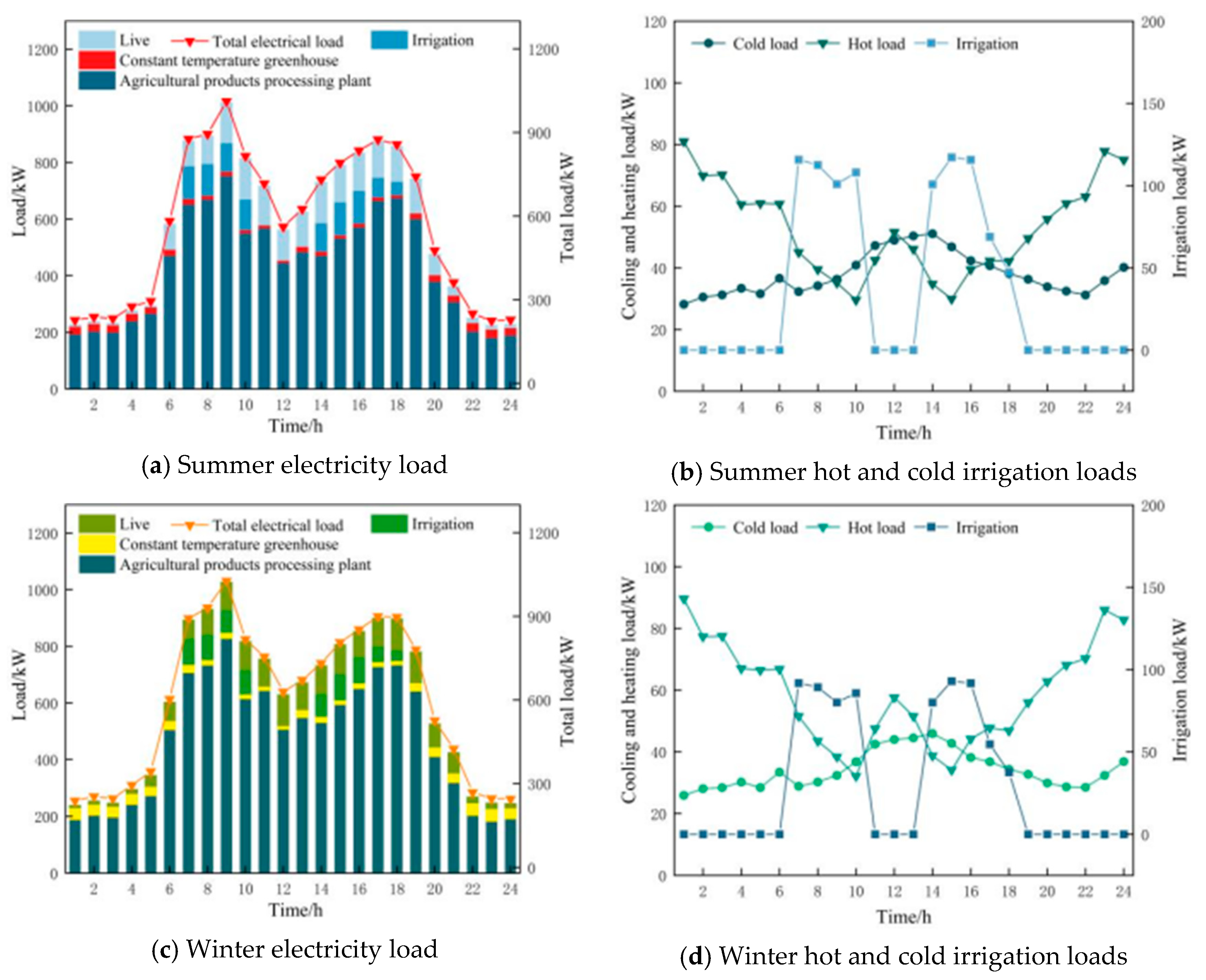
Figure 10a–d are the cooling, heating, and electricity load data on typical days in summer and winter after all types of loads participate in demand response.
As shown in Figure 10a, agricultural product processing plants are the main component of the electricity load in each period, followed by rural life load and irrigation load. Constant temperature greenhouses require the least electricity load due to their simple energy use form. Compared with Figure 10c, it can be seen that the electricity load demand of constant temperature greenhouses has increased. This is because the temperature is low in winter, and the constant temperature greenhouse needs to increase energy demand to maintain a constant temperature state. By comparing Figure 10b,d, it can be seen that rural areas have higher irrigation and cooling load demands in summer than in winter. This is because the weather is hot and the temperature is high in summer, and the water evaporation is large. Agricultural irrigation and cold storage need to increase energy to maintain their load demand. At the same time, the heat load demand of agricultural product processing plants in winter is also increasing compared to summer.
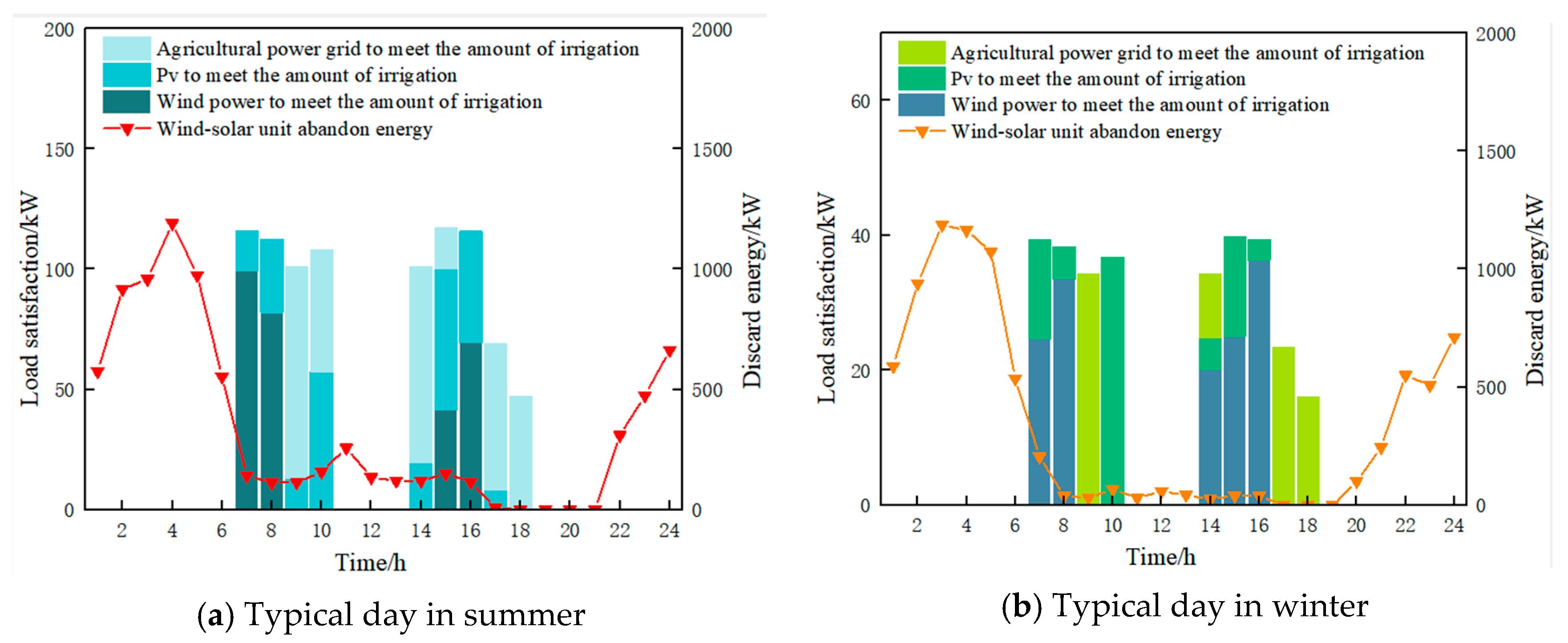
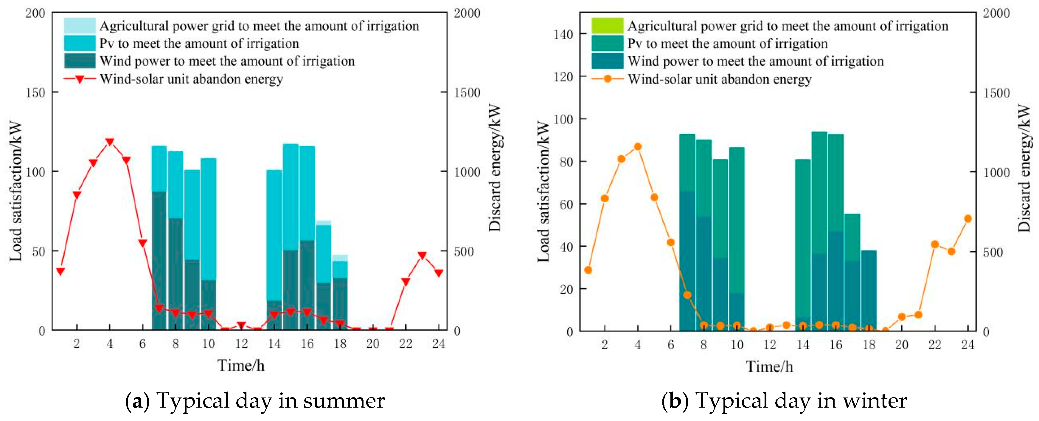
Figure 11 shows the optimization results of the CES for rural irrigation energy use on typical days in summer and winter and the wind and solar energy abandonment of the CES.
The consumption of clean energy on typical days in summer and winter is shown in Figure 11. As shown in Figure 11a,b, in addition to describing the consumption of wind and solar resources, it also shows the dispatch of each unit to meet the irrigation volume. During the nighttime period of 3:00–5:00, wind turbines generate a large amount of abandoned energy. This is due to the low demand for daily energy consumption of villagers and direct electricity load in the production park at night, and the abundant wind power resources at night. The low-carbonization degree of the clean energy system is high during this period. During the period of 9:00–17:00, the system requires high cooling and heating loads and electricity loads, so the wind and solar units have less abandoned energy and a higher consumption rate. At the same time, the clean energy system purchases electricity from the rural grid to meet the remaining load demand. The irrigation load during the period of 17:00–18:00 is mainly met by the rural grid. This is because this period is close to dusk, the photovoltaic power generation is reduced, and the heat load demand of the industrial park continues to increase. Therefore, the clean energy system purchases electricity from the rural grid to meet the remaining load. During the period of 6:00–8:00 and 16:00, the irrigation load is fully met by clean energy, achieving comprehensive low carbonization and creating benefits for the clean energy system. Comparing Figure 11a,b, it can be seen that the energy required for irrigation in winter is relatively low in the rural power grid. This is because the irrigation demand is low during the entire scheduling cycle in winter, so the amount of electricity purchased by the CES from the rural power grid is relatively low, and the economic benefits of the CES in the typical winter scenario are relatively high.

5.3.4. Analysis of the Results of Scenario 3

Introducing energy storage devices based on the response of various load demands in Scenario 2, energy storage aggregators obtain benefits by buying at low prices and selling at normal prices, while optimizing the new energy consumption rate during the operation of the CES. The scheduling results of Scenario 3 are shown in Table 7. The low-carbonization degree of the CES on typical summer and winter days is improved by 365.29 and 323.11 compared with Scenario 2, and the economic income of the CES is increased by CNY 5966.34 and CNY 5586.9. It can be seen from the scheduling results that the low-carbonization degree index of the CES on typical summer days is higher than that of typical winter days, while the economic benefit index is lower than that of typical winter days.
The main costs of the CES during the dispatch cycle after the introduction of energy storage devices are shown in Table 8. Due to the large overall demand for irrigation load, cooling load, and living energy on typical summer days, the CES needs to purchase electricity from energy storage aggregators and rural power grids during certain periods, with purchase costs of CNY 554.32 and CNY 87.35, respectively. Therefore, the cost of purchasing electricity from external sources in summer is relatively high compared to winter, and the equipment depreciation cost is also higher. This is one of the reasons why the economic benefits of the CES on typical summer days are lower than those on typical winter days.
The optimized dispatch of the CES in a typical day is divided into two situations: living energy and production energy. The specific optimization results are as follows.
(1) Optimization results of living energy
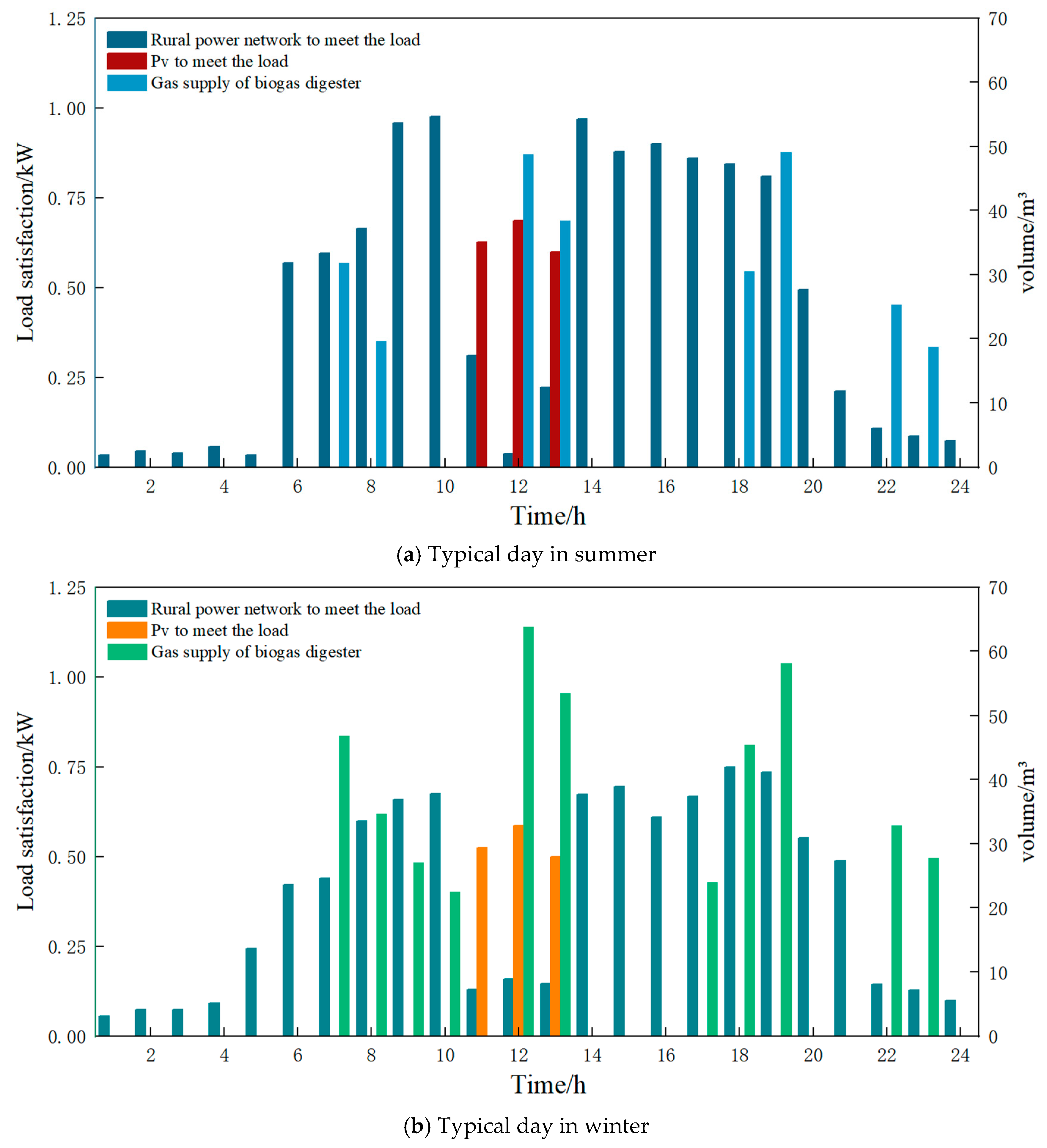
The daily energy supply and consumption of rural villagers in summer and winter are shown in Figure 12a,b. The living electricity consumption is calculated per household, while the biogas demand is based on the entire village. Due to the regularity of rural living habits, electricity consumption is relatively low before 6:00 AM and after 8:00 PM, with peak electricity demand occurring between 9:00 AM and 7:00 PM. The biogas in the CES is directly used to meet the villagers’ daily cooking needs without being converted into electricity. The peak biogas demand period is from 12:00 PM to 1:00 PM and 6:00 PM to 7:00 PM. The daily cooling and heating load demand is met by the conversion unit in the CES. From 11:00 AM to 1:00 PM, photovoltaics supply the main electricity load demand, while the electricity load during the remaining periods is met by the rural power grid. Comparing Figure 12a,b, it can be observed that the demand for cooking, heating, and lighting in winter is higher, resulting in greater biogas and electricity load demand in winter than in summer.
In summary, compared with the original rural energy supply, the introduction of clean energy significantly enhances the low-carbon level of living energy use, while also providing economic benefits for the clean energy system.
(2) Optimization results of production energy consumption
The CES provides energy for rural industrial parks. At the same time, various loads influence the optimization scheduling of CES units through response methods such as whole-section shifting, scattered scheduling, and peak reduction. The optimization results of production energy consumption in rural industrial parks are shown in Figure 13, Figure 14, Figure 15, Figure 16, Figure 17, Figure 18, Figure 19 and Figure 20.
The optimization results of CES production energy consumption on typical days in summer and winter are shown in Figure 13a,b. Wind and solar energy meet most of the production electricity demand. As shown in Figure 13a, during the period of 17:00–18:00 on a typical summer day, wind and solar units, biogas turbines, and rural power grids jointly meet the remaining electricity load demand. This is because the output of wind and solar units meets the high demand for cooling, heating, and irrigation loads during this period. During this time, the output of wind and solar units is almost entirely consumed, and the CES purchases electricity from the rural power grid to meet the remaining load. Throughout the scheduling period, biogas turbines meet a lower electricity load than wind and solar units. This is because the output of wind and solar units has a certain randomness and uncertainty. In order to ensure the environmental protection and economy of the CES, wind and solar resources are prioritized. Electric refrigeration units and electric boilers meet the cooling and heating loads, respectively, so their power consumption curves are consistent with the cooling and heating load curves. As shown in Figure 13b, on a typical winter day, except for the reduction in energy consumption of electric refrigeration machines, the other load demands all increase. At the same time, due to the higher wind power output in winter, the load satisfied by wind and solar power on a typical winter day increases, while the load satisfied by the biogas unit decreases. Consequently, the CES does not need to purchase electricity from the rural grid.
The optimization results of the CES satisfying the cooling and heating loads on typical days in summer and winter are shown in Figure 14a,b. In the 11:00–12:00 period of Figure 14a, clean energy meets a relatively low heat load throughout the entire dispatch period, with the heat load mainly being met by wind turbines through electric refrigeration machines. In the 14:00–16:00 period, the cooling load is met by biogas units. This is because the output from wind and solar power is nearly fully absorbed during this period. In Figure 14b, during the 8:00–11:00 period and the 13:00–16:00 period, wind power hardly meets the cooling and heating loads. During these periods, the cooling and heating loads are instead met by other clean energy units. This is due to the system’s electrical load being at a peak during this time and wind power resources being limited.
Figure 14. Cooling and heating load optimization results.
Processes 13 01366 g014
In the periods of 1:00–6:00 and 22:00–24:00 in Figure 14a, and 0:00–5:00 and 20:00–24:00 in Figure 14b, the cooling and heating loads are fully met by clean energy, achieving comprehensive low carbonization. As can be seen from both figures, the energy abandonment of wind and solar units increases during the 22:00–24:00 period, which sufficiently demonstrates the abundance of clean energy during this time. As a result, the cooling and heating loads are met in this period, ensuring comprehensive low carbonization.
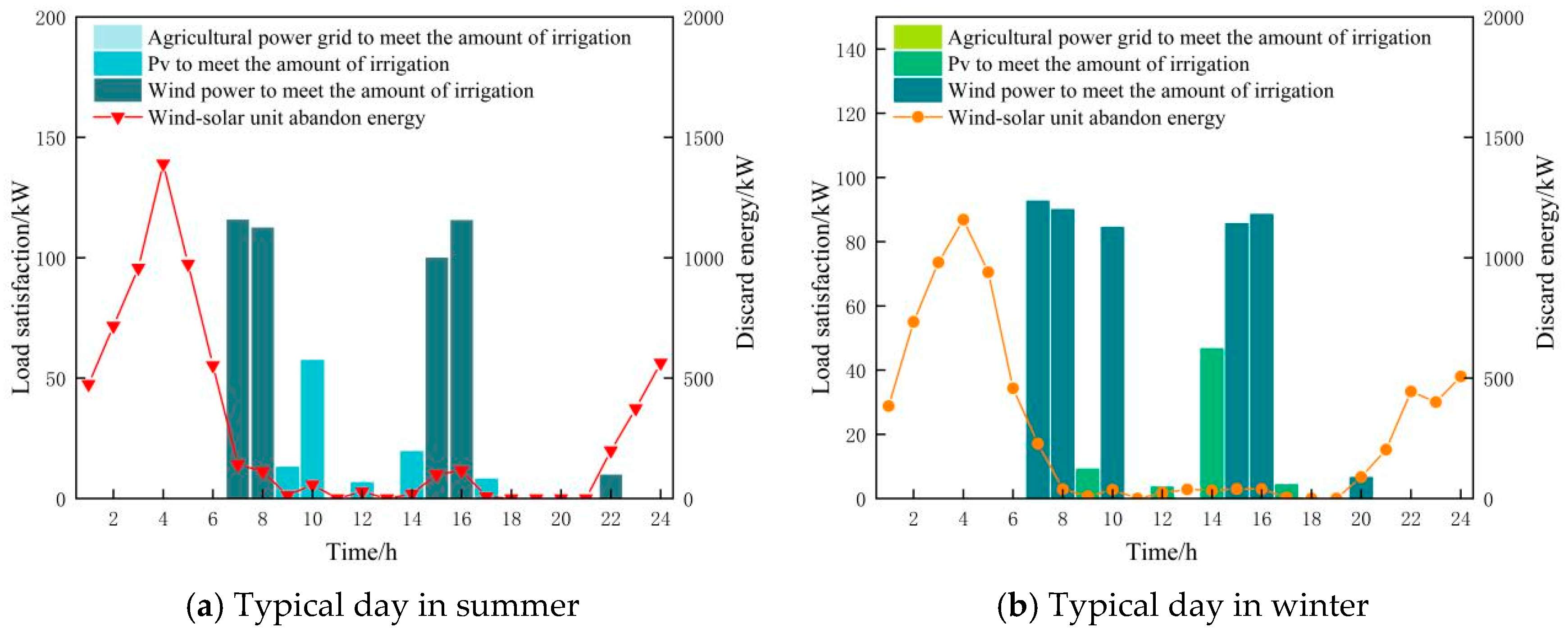
The consumption of clean energy in typical days during summer and winter in Scenario 3 is shown in Figure 15. As illustrated in Figure 13a,b, during the nighttime period of 3:00–5:00, wind turbines generate a large amount of abandoned energy, and the low-carbonization degree of the CES reaches its highest level during this period. In Figure 15a, from 9:00 to 17:00, the abandoned energy of the CES wind and solar units is relatively small. During the period of 17:00–18:00, the CES purchases electricity from the rural power grid to meet the remaining load demand, with the irrigation load mainly supplied by the rural power grid and wind power. This is because this period is close to dusk, photovoltaic power generation decreases, and the heat load demand of the industrial park continues to rise. As a result, the CES purchases electricity from the rural power grid to fulfill the remaining load demand. In other periods, the irrigation load is fully met by clean energy, achieving comprehensive low carbonization and generating benefits for the CES. As shown in Figure 15b, the abandoned energy in winter is higher than in summer throughout the entire scheduling period, with wind power abandonment being more pronounced during the 20:00–24:00 period.
Figure 15. Irrigation energy consumption and clean energy consumption results.
Processes 13 01366 g015
Comparing Figure 15 and Figure 11, the total amount of wind and solar energy abandonment on typical days in summer and winter in Scenario 3 with the introduction of energy storage is less than the total abandoned energy in Scenario 2. This is because energy storage aggregators will purchase at low prices during periods of high abandoned energy and sell at normal prices when the CES needs to purchase electricity, thereby earning profits while improving the low-carbonization degree of the CES.
Figure 16a,b show the operating status of energy storage devices in Scenario 3 on typical days in summer and winter, respectively.
Figure 16. Energy storage operation status.
Processes 13 01366 g016
As shown in Figure 16a,b, on typical days in different seasons, the energy storage device in the CES exhibits noticeable differences in charge and discharge patterns in response to changes in load demand and wind and solar resources. These differences highlight the critical role of energy storage in balancing energy supply and optimizing economic objectives. On typical summer days, the frequency and total amount of charge and discharge by the energy storage devices are relatively high. During the period of 3:00–8:00, the energy storage device remains in a state of continuous, small-scale charging. This phase corresponds to the nighttime period when wind power resources are abundant, but the load demand of the system is low, leading to the abandonment of some wind power resources. To avoid wasting this surplus energy, the CES stores the excess wind power through energy storage devices, thereby enhancing the utilization rate of wind power.
During the high-load periods of 9:00–11:00, 14:00–15:00, and 17:00–19:00, the energy storage system is continuously discharged. During these times, the load demand is high, and the available wind and solar resources are insufficient to meet the system’s requirements. The CES draws electricity from the energy storage device, which not only reduces the cost of electricity purchases but also helps to meet peak load demands, thus improving the overall economy of the system. In the period of 22:00–23:00, when wind power resources are abundant again and system load demand is relatively low, a significant amount of energy is abandoned. During this time, the CES purchases electricity at a low price and stores it, with the charging power of the energy storage system increasing substantially. This charging strategy effectively leverages the low electricity prices during off-peak hours and the abundant wind resources, thereby enhancing the efficiency of wind energy utilization.
On a typical winter day, the charging and discharging characteristics of energy storage are different from those in summer. First, during the period of 11:00–13:00, after the energy storage system has undergone a large amount of charging, it enters a 2 h small amount of charging stage. The reason for this phenomenon is that there is no irrigation load during this period, the overall load demand of the system decreases, and the abandoned energy increases. The CES chooses to store part of the abandoned energy. At the same time, the SOC of the energy storage device is close to saturation, so it enters a small amount of charging mode during the period of 12:00–13:00 to maintain battery health. During the period of 14:00–20:00, the energy storage continues to discharge. At this stage, the system’s cooling, heating, and electricity loads are all at peak, and the wind and solar resources are fully absorbed. The energy storage discharge helps to meet the peak load demand and reduce the pressure of external power purchase. Entering the nighttime period (20:00–23:00), wind power resources are abundant again, the load is low, and the energy storage device resumes charging, further improving the new energy consumption capacity of the CES and reserving sufficient electricity for the next dispatch cycle.
By comparing the energy storage operation characteristics on typical summer and winter days, it is evident that both the amount and frequency of energy storage charging and discharging are significantly higher in summer than in winter. This discrepancy is primarily due to the higher volatility of load demand during the summer months, combined with the weaker stability of wind and solar resources, particularly wind power. As a result, energy storage devices are required to charge and discharge more frequently in order to balance the load. In contrast, during the winter, wind power resources are more abundant, and the load demand is relatively stable. Consequently, the CES relies less on energy storage for electricity procurement, leading to a reduction in the frequency of charging and discharging events.
Overall, the integration of energy storage devices into the CES system has significantly enhanced the degree of low carbonization. The energy storage system is capable of flexibly charging and discharging in response to fluctuations in load demand and electricity market prices, which not only reduces reliance on external electricity sources but also mitigates the impact of peak load on the system. By capturing and storing wind and solar surplus energy, the system reduces renewable energy waste while simultaneously improving its economic performance. The real-time responsiveness of the energy storage device allows the CES to effectively manage the volatility and uncertainty associated with wind and solar power generation, optimizing resource utilization and boosting overall system efficiency.

5.3.5. Analysis of the Results of Scenario 4

Building upon the introduction of energy storage in Scenario 3, Scenario 4 introduces a high-level water tower, which is integrated with a drip irrigation system to fulfill irrigation requirements. The high-level water tower operates by using a water pump to store water during periods when the system energy supply is adequate, and releases water during irrigation periods. This coordinated operation with drip irrigation ensures efficient irrigation water supply. The scheduling results for Scenario 4 are presented in Table 9. Compared to Scenario 3, the degree of low carbonization and economic benefits of the CES on a typical summer day are 4.32% and 2.18% higher, respectively, while on a typical winter day, the degree of low-carbonization and economic benefits are 3.94% and 3.34% higher. Notably, the low-carbonization degree and system economic benefits for a typical winter day exceed those of a typical summer day.
The main costs of the CES during the dispatching cycle, after the introduction of the high-level water tower, are shown in Table 10. The integration of the high-level water tower significantly improves the energy utilization rate of the CES. As a result, the cost of purchasing electricity from the rural power grid during the entire dispatching cycle of the CES on typical days in both summer and winter is reduced to zero. The cost of purchasing electricity from energy storage amounts to CNY 183.95 in summer and CNY 115.6 in winter, both of which are substantially lower than the electricity purchase costs from energy storage in Scenario 3. This reduction is attributed to the high-level water tower’s ability to decrease the frequency and volume of energy storage charging. Additionally, the water release for irrigation from the high-level water tower reduces the CES’s reliance on electricity from energy storage, further lowering the overall electricity purchase costs. Despite this, the overall load demand for various energy types on typical summer days remains high, which results in a relatively higher cost in summer. Consequently, the system’s economic benefits are slightly lower in summer than in winter.
Figure 17 shows the satisfaction of irrigation load demand in summer and winter and the optimization results of irrigation load and compares the energy abandonment of wind and solar units in summer.
Figure 17. Irrigation energy consumption and clean energy consumption results.
Processes 13 01366 g017
The consumption of clean energy on typical days in summer and winter in Scenario 4 is shown in Figure 17. As illustrated in Figure 17a,b, the CES no longer purchases electricity from the rural grid to meet the irrigation load on typical days in both summer and winter. This is due to the high-level water tower’s water storage and drainage irrigation method, which fully satisfies the irrigation demand, thereby eliminating the need for electricity purchases from the rural grid. When comparing Figure 17 with Figure 15, which represents Scenario 3 where energy storage is introduced, it can be observed that the total amount of wind and solar energy abandonment on typical days in both summer and winter is lower in Scenario 4. This improvement is because the high-level water tower utilizes periods of high wind and solar energy abandonment to pump and store water. During irrigation periods, the water tower releases water to meet the irrigation demand, thus reducing the electricity load required for drip irrigation. This approach not only decreases the reliance on electricity but also enhances the utilization of wind and solar resources, leading to improved low carbonization of the system.
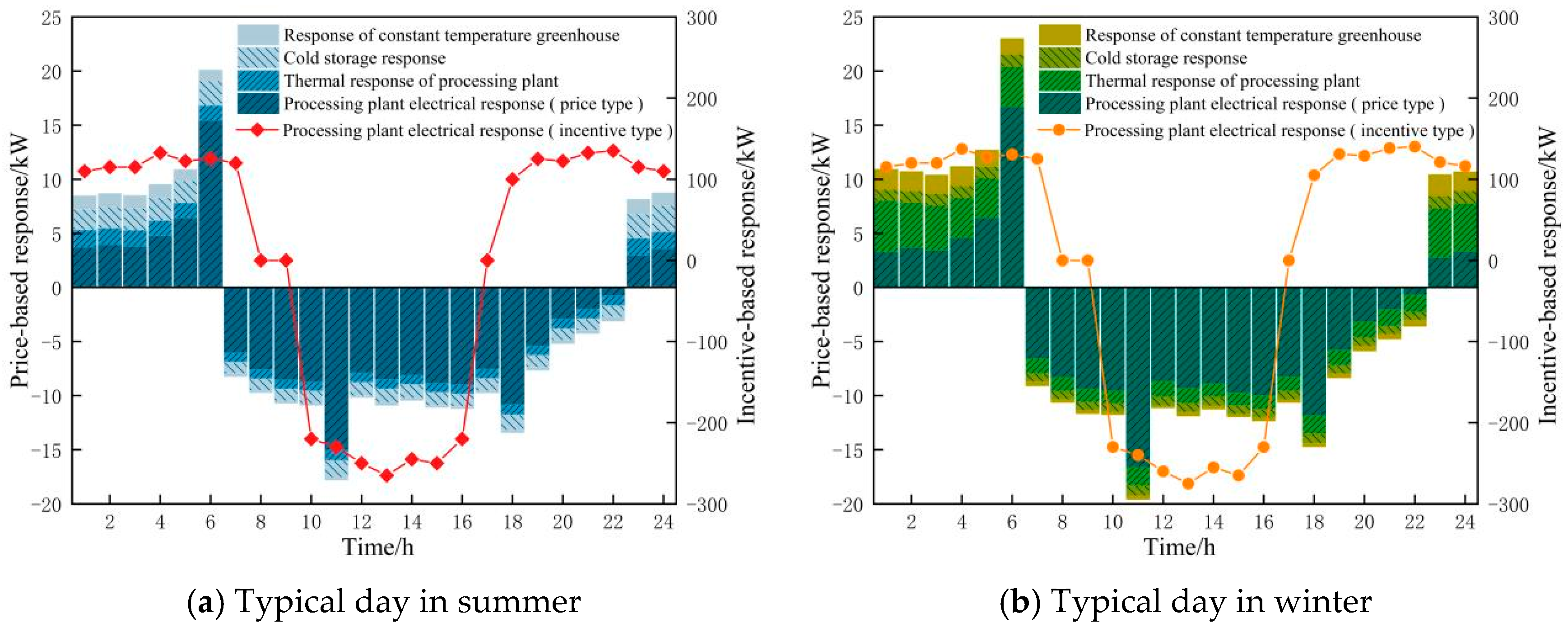
Figure 18 summarizes the response of various production loads in summer and winter under different participation methods.
Figure 18. Production load response scheme.
Processes 13 01366 g018
In the summer, the load response is more pronounced during the 8:00–18:00 period, primarily due to the high daytime temperatures, which lead to increased cooling demand for cold storage and constant-temperature greenhouses. Additionally, the power load of the processing plant is also influenced by temperature fluctuations and production demands. In terms of price response, cold storage exhibits a more significant response during the day, as it increases electricity consumption to maintain the required temperature, while reducing load during periods of higher electricity prices (8:00–10:00, 14:00–16:00). Moreover, the incentive response is more active during the day in summer, particularly around 14:00 when the power load of the processing plant is most influenced by the incentive-based response. The price response of the processing plant’s power load is more substantial during the 6:00 and 11:00 periods, as the electricity prices in these periods are the lowest and highest, respectively, making the response more noticeable.
The load response in winter exhibits distinct characteristics compared to summer. The price response during the day is not as pronounced as in summer, and there is an increase in load during the night (18:00–24:00). This is primarily due to the lower temperatures at night in winter, which necessitate an increase in the heat load of constant temperature greenhouses and cold storage to maintain a stable temperature. Furthermore, the incentive response is more noticeable during the morning and evening peak periods. Specifically, the processing plant shows a larger response around 6:00 in the morning and 18:00 in the evening, helping to alleviate the morning and evening peak load demand. Comparing Figure 18a,b, it is evident that the cooling load demand of cold storage on a typical summer day is higher than on a typical winter day, resulting in a greater cooling load response in summer. Conversely, the heating load required by the agricultural product processing plant on a typical winter day exceeds that of a typical summer day, so the heat load response of the processing plant in winter is also higher than in summer.
The constant-temperature greenhouse exhibits load response in both seasons, though the heat load demand is more pronounced in winter to maintain the necessary temperature for plant growth. The price-response strategy reduces energy consumption during the day and supplements it during the low electricity price period at night. The response pattern of cold storage differs significantly between summer and winter. In summer, the cooling demand during the day is higher, so the load response of cold storage is mainly concentrated during periods of low electricity prices, with the electricity price used as an incentive to increase the load. In winter, due to the lower ambient temperature, the load demand of cold storage decreases, leading to a reduced response intensity. The response of the processing plant is influenced by both price and incentive factors, displaying a diurnal periodic fluctuation. In summer, the power load response of the processing plant is more concentrated during the daytime, while in winter, it is primarily guided by incentives during the morning and evening, offering greater flexibility in its response.
It can be observed that the production load response strategies in both summer and winter effectively contribute to reducing peak power demand, smoothing the load curve and alleviating the operating pressure on the power grid. By optimizing electricity usage during low-electricity-price periods and minimizing consumption during high-price periods, this load response mechanism enhances the economic efficiency of the system. Additionally, the role of incentive-based responses is particularly significant during critical periods, further improving the effectiveness of load adjustments and adapting to seasonal variations. The implementation of this load response scheme aligns with the goal of promoting the consumption of clean energy. By increasing the load during low-electricity-price periods, the system maximizes the utilization of renewable energy and reduces reliance on rural power grids. Furthermore, the incentive response helps to guide the power consumption of the processing plant during periods of high wind and solar power generation, thereby enhancing the efficiency of clean energy use. These response schemes are tailored to the specific characteristics of rural loads, developing practical and feasible strategies based on their particular load demands. In contrast to the general approach in the literature [17], which typically categorizes loads as simple electric loads for demand response, this approach is more practical and better suited to the unique conditions of rural areas.
Figure 19 illustrates the operating status of the high-level water tower and the irrigation water supply situation, depicting the fulfillment of irrigation load demands in both summer and winter. It also provides a detailed view of the operational status and water storage capacity of the high-level water tower during each period. This visual representation showcases how the high-level water tower effectively meets the irrigation needs by utilizing stored water during peak irrigation periods, thus optimizing water usage while reducing the dependency on electricity for irrigation purposes. The data also highlight the tower’s performance across different seasons, reflecting its contribution to improving energy utilization and system efficiency.
Figure 19. High-level water tower operation status and irrigation water supply.
Processes 13 01366 g019
As shown in Figure 19a, during a typical summer day, the high-level water tower operates with a low flow rate, performing small-scale pumping from 1:00 to 7:00 to replenish the water level. During the irrigation periods of 9:00 to 10:00, 14:00 to 15:00, and 17:00 to 18:00, the water tower discharges water to meet the irrigation demand. However, the water supply from the water tower during these periods does not fully satisfy the irrigation load, and additional irrigation demand is partially supplemented by drip irrigation. Additionally, the pumping volume of the water tower increases significantly during the 12:00 and 22:00 periods due to low electricity prices, which helps to reduce the operating costs of the water pump. Moreover, at the 22:00 period, abundant wind power abandonment occurs within the CES system, and the water tower’s pumping operation effectively utilizes this low-cost clean energy to store water for subsequent irrigation needs.
As shown in Figure 19b, the amount of water pumped and drained by the high-level water tower on a typical winter day is lower than that on a typical summer day. During a typical winter day, the water tower continuously pumps a small amount of water from 1:00 to 7:00, drains water from 14:00 to 18:00 to meet irrigation needs, and pumps water until the water tower is full from 20:00 to 24:00. These operations are planned considering the abandonment of wind and solar energy and the electricity costs in each period. The operation strategy of the high-level water tower depends on the dynamic changes in electricity prices and the availability of wind and solar energy. By storing water during low-electricity-price periods, the system effectively utilizes wind and solar energy abandonment and reduces energy waste. On the other hand, draining water for irrigation during high-electricity-price periods not only satisfies the irrigation demand but also helps to avoid increased costs during peak periods. This strategy optimizes the efficiency of resource utilization, enhances the absorption rate of clean energy in the system, and ultimately brings significant economic benefits to the CES system.
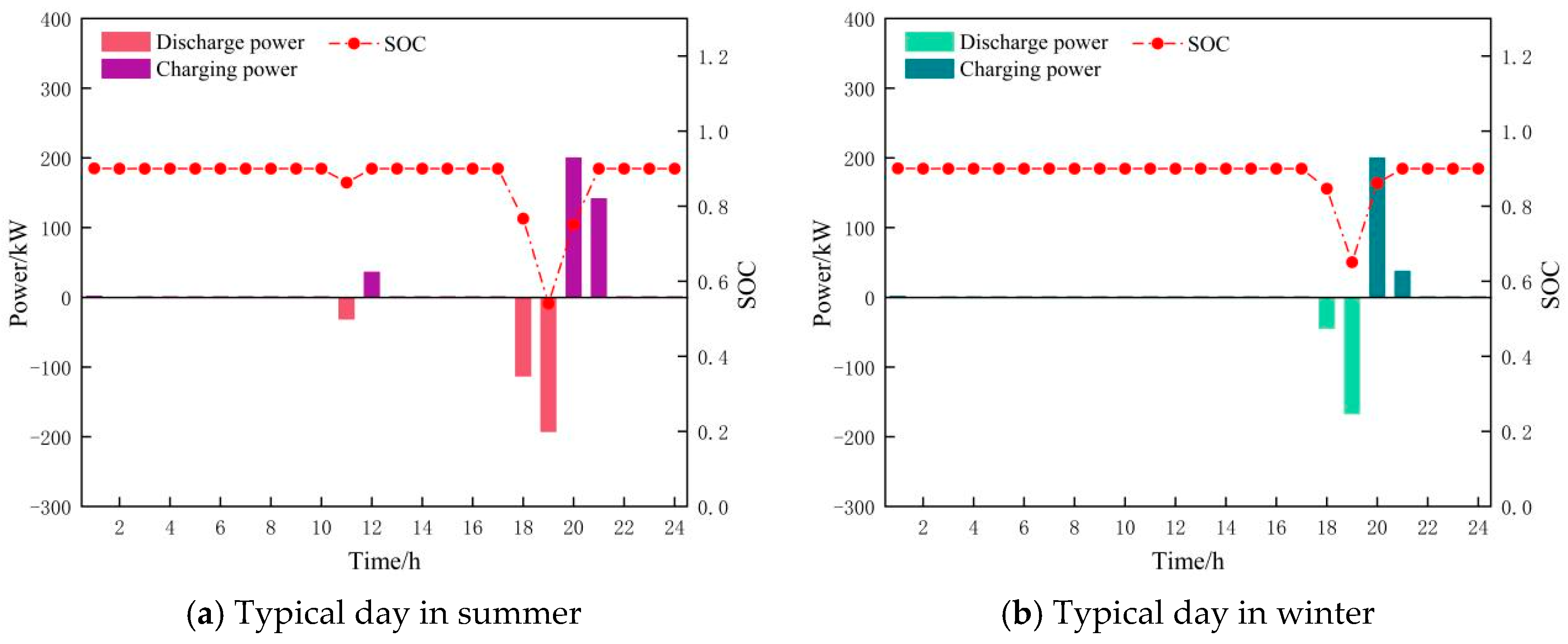
Figure 20 illustrates the charging, discharging, and state of charge of the energy storage system at different times of day during both summer and winter and compares the operational differences between the two seasons.
Figure 20. Energy storage operation status.
Processes 13 01366 g020
Figure 20 shows the different response strategies of the energy storage system in summer and winter. In summer, the energy storage system balances the load by charging during low-load periods and discharging during high-load periods, reducing the need for electricity purchases. In winter, the system’s reliance on energy storage decreases due to the abundance of wind power resources. In Scenario 4, where a high-level water tower is introduced, the energy storage system is further optimized, reducing electricity purchase costs and increasing the absorption of clean energy.
Figure 20a shows that the energy storage system performs minimal charging operations from early morning to morning in summer (3:00–10:00), mainly due to low load demand at night and surplus wind and solar resources. The system charges during this period to provide power reserves for subsequent high-load periods. From morning to noon (11:00–12:00), the system exhibits alternating charging and discharging behavior, reflecting the volatility of electricity loads during this time. Around 11:00, the load is high, and the system relies on energy storage to balance the short-term power gap. At 12:00, the irrigation load temporarily disappears, increasing the amount of abandoned energy, which the energy storage system utilizes to charge. Simultaneously, the water tower pumps and stores a large amount of water, making full use of excess electricity for peak shaving and valley filling. During the evening peak period (18:00–19:00), the system load demand peaks for the day. With wind and solar resources nearly depleted, the energy storage system discharges a large amount to supplement the load demand and alleviate system pressure, ensuring stable electricity supply. During the night period (20:00–24:00), as the load demand gradually decreases and abandoned wind and solar energy increases, the energy storage system charges to utilize low-cost excess clean energy. Additionally, the high-level water tower stores water during this time to prepare for future demand. This charging and discharging strategy in summer enables flexible response during peak load periods and reserves electricity during valley periods, optimizing the system’s economic benefits.
As shown in Figure 20b, the overall charge and discharge volume decreases in winter, primarily due to the relatively abundant wind power resources. The output of wind power can better meet load demand, reducing the need for the CES system to purchase electricity from energy storage aggregators. Compared to summer, the energy storage system in winter has a reduced charging period at night, as wind resources are more stable, allowing the system to rely more directly on wind power during the day, thereby reducing the need for charging. At the same time, the increase in load demand during winter has limited the discharge demand of the energy storage system during the evening peak, reflecting the change in reliance on energy storage at different times. In comparison to Scenario 3, Scenario 4, which introduces a high-level water tower, demonstrates a significant optimization of energy storage. The high-level water tower allows the CES system to store excess clean energy during low-electricity-price periods and release it when irrigation loads occur, providing auxiliary support to the system. This configuration improves the clean energy utilization rate and reduces the need for the CES to purchase electricity from energy storage aggregators. High-level water towers not only reduce the frequency of energy storage system charging and discharging but also decrease the cost of electricity purchases by regulating part of the irrigation load through water, thus improving the economic benefits of the CES. Additionally, due to the water tower’s regulation capacity, the energy storage system can reduce deep discharges, extend battery life, and further lower operating costs.
Based on the above analysis, in terms of carbon emission reduction, the low-carbonization degree in both summer and winter of the baseline scenario is not negative. After the introduction of the CES, the low-carbonization degree gradually increases and decreases with the expansion of system considerations. Among these, Scenario 2 performs better than Scenario 1, with the low-carbonization degree on typical summer days increasing by 108%. Scenario 4 achieves the highest low-carbonization degree after the introduction of high-level water towers. Economically, the baseline scenario results in negative returns, while Scenarios 1 and 2 yield lower returns. Scenario 3 shows a significant improvement over Scenario 2, and Scenario 4 maximizes economic benefits. Therefore, the optimization plan in Scenario 4 is prioritized.

5.3.6. Wind and Solar Output Sensitivity Analysis

In summary, since Scenario 4 is the optimal solution, this section uses Scenario 4 as an example to conduct a sensitivity analysis of wind and solar output. The sensitivity analysis results of wind speed and solar radiation intensity on a typical CES summer day are shown in Figure 21.
The results of the sensitivity analysis on typical summer days indicate that wind speed and solar radiation intensity are essentially linearly correlated with the low-carbonization degree and economic benefits of the CES optimization model. Specifically, an increase in these two variables leads to an increase in both the low-carbonization degree and economic benefits. On typical summer days, when the wind speed varies within a reasonable range, the maximum change in the low-carbonization degree of the CES is 2.08%, while the maximum change in economic benefits is 2.81%. When the solar radiation intensity varies within a reasonable range, the maximum change in the low-carbonization degree of the CES is 2.74%, and the maximum change in economic benefits is 1.45%. Sensitivity analysis for typical winter conditions reveals a strong linear relationship between wind speed/solar radiation intensity and both decarbonization performance and economic benefits in the CES optimization model as demonstrated in Figure 22.
Within operational limits, wind speed variations cause maximum fluctuations of 1.77% in the decarbonization rate and 2.64% in economic benefits, while solar radiation intensity changes lead to 2.9% and 1.86% variations in these respective parameters.
In summary, the uncertainty associated with wind and solar power generation results in variations below 5% for both the decarbonization level and economic benefits of the CES system during typical seasonal operation, confirming the model’s robust performance characteristics.

6. Conclusions and Outlook

This study develops a rural clean energy supply system framework aligned with national rural revitalization and carbon neutrality goals. The proposed system addresses three primary energy demand sectors—residential consumption, agricultural production, and irrigation requirements—with production loads specifically including agricultural processing plants, cold storage facilities, and temperature-controlled greenhouses. Using a novel decarbonization assessment model, we quantitatively evaluate the CES’s emission reduction potential while simultaneously optimizing its economic performance. Our comprehensive analysis, combining theoretical modeling and empirical case studies, yields the following key findings:
(1) When implementing the demand response (DR) policy, the distributed clean energy system guides load adjustment through price signals, with different load types exhibiting distinct response patterns. The results show that compared to non-DR scenarios, the decarbonization level increases by 2563.08 units in summer and 785.11 units in winter, while economic benefits increase by CNY 113.2 and CNY 617.75, respectively. The DR mechanism not only enhances the low-carbon effect of the CES but also significantly improves its economic performance by optimizing the matching between load demand and renewable energy supply. This approach effectively reduces dependence on external power during peak periods while maximizing utilization of low-cost electricity during off-peak times (Appendix A).
(2) This paper proposes a robustness coefficient to mitigate and manage the impact of energy supply uncertainty on the operation of clean energy systems (CES). An increase in the robustness coefficient leads to a reduction in clean energy output, thereby lowering the operational risk of the CES. However, this may also result in diminished economic returns. Consequently, it is essential to strike an appropriate balance between system robustness and economic performance by selecting an optimal robustness coefficient. The proposed robustness strategy enables the CES to operate reliably under uncertain conditions, ensuring that the system maintains a desirable equilibrium between low carbon emissions and economic benefits, even amidst significant fluctuations in resource availability.
(3) Based on annual data for cooling, heating, and electricity loads, this study employs an ordered clustering method to analyze load characteristics. The silhouette coefficient is utilized to determine the optimal number of segmentation points, enabling the extraction of representative scenarios across different seasons and load profiles. This classification of typical scenarios simplifies the original load data and allows for a more accurate representation of energy demand across time periods in simulation studies. By aligning with seasonal variations in load characteristics, the CES can implement more flexible and adaptive energy supply strategies, thereby enhancing overall energy utilization efficiency.
(4) The energy storage system (ESS), characterized by its flexible charging and discharging capabilities, effectively accommodates surplus wind and solar power, mitigating renewable energy curtailment. It supports the energy supply of the CES during peak load periods, reduces reliance on external electricity purchases, and substantially enhances the system’s level of decarbonization. Compared to scenarios employing demand response alone, the integration of ESS increases the CES’s decarbonization level by 365.29 and 323.11 units in summer and winter, respectively. Furthermore, economic benefits are improved by CNY 5966.34 and CNY 5586.90 in the respective seasons. These results demonstrate that the incorporation of ESS significantly enhances the operational flexibility and overall performance of the CES.
(5) Irrigation energy constitutes a significant component of rural energy demand and exhibits strong seasonal variability. To further optimize irrigation load management, this study incorporates the use of elevated water towers—commonly found in rural areas—within the CES framework. These water towers serve dual functions: meeting agricultural irrigation needs and mitigating the uncertainty of wind and solar power output. Specifically, water pumps store water during periods of excess renewable energy (i.e., high curtailment), and release it during irrigation periods, thereby reducing the direct electricity demand for irrigation. This approach not only enhances the energy utilization efficiency of the CES, but also lowers electricity procurement from the external grid during irrigation seasons, effectively reducing energy supply costs. The results indicate that the integration of elevated water towers increases the decarbonization level of the CES by 4.32% and 3.94% on typical summer and winter days, respectively, while the overall economic benefits improve by 2.18% and 3.34%. The application of elevated water towers thus enables the CES to reduce peak-period grid dependency and improve overall economic performance.
(6) This study selects a rural area in Guanzhong, Shaanxi Province, China, as a representative case study. To ensure adaptability to varying geographical and socio-economic conditions, it is essential to fully consider regional differences, including topography, water resources, and climate. In mountainous rural areas with significant elevation changes, elevated water towers can utilize gravity for water delivery, thereby reducing the energy required for pumping and enhancing overall system efficiency. In flat areas, water towers rely primarily on external energy sources, such as photovoltaics and water pumps, to elevate water, making it necessary to optimize pump operation strategies—such as using locally available PV and wind power—to reduce the reliance of the CES on electricity purchased from the rural grid. In regions with abundant water resources, the CES can integrate small-scale hydropower stations or rainwater-harvesting systems with water towers to establish a complementary water supply system, improving water resource utilization. In contrast, in areas with scarce water availability, it is crucial to plan water storage and dispatch strategically, optimize the operational model of elevated water towers, and incorporate water-saving irrigation technologies to minimize losses. In solar-rich regions, the extensive deployment of rural PV systems can drive water pumps efficiently when coupled with energy storage to optimize electricity use. In cold-climate regions, appropriate insulation measures are needed to prevent freezing of water towers in winter, which would otherwise increase the CES load. In economically advanced rural areas, intelligent control systems can be introduced to enable accurate load forecasting and optimized scheduling, whereas in less-developed regions, low-cost configurations such as PV combined with elevated water tower-based energy storage offer practical alternatives. In areas where electricity prices are high, operational strategies involving peak shaving and valley filling can be employed to effectively reduce overall energy costs.
(7) The combination of elevated water tower supply technology and photovoltaic water extraction is technically feasible, as both technologies have been widely implemented in practice. By optimizing system operation through peak shaving and valley filling strategies, peak electricity consumption can be effectively reduced, thereby lowering rural electricity costs. From an economic perspective, the use of renewable energy sources such as photovoltaics reduces dependence on fossil fuels and enhances long-term economic returns, demonstrating the economic viability of the proposed model. Additionally, distributed energy technologies—such as photovoltaics, wind power, and small-scale hydropower—are supported by national renewable energy subsidy programs, and in some regions, agricultural photovoltaic projects are eligible for further financial incentives. Furthermore, under the rural revitalization policy, the development of rural energy infrastructure is strongly encouraged. As such, the proposed plan aligns with national strategic goals and possesses strong policy feasibility.
(8) To accelerate rural energy transformation and facilitate the widespread adoption of the community energy system (CES) model, the following policy recommendations are proposed. First, green carbon-trading incentives should be established by incorporating elevated water tower energy storage systems into the national carbon trading framework. Rural users can benefit from carbon credit revenues by reducing reliance on fossil fuels, with estimated trading returns of CNY 30–50 per ton of carbon emissions reduced. Enterprises should be encouraged to invest in rural water tower energy storage projects and include them as carbon offset initiatives, enabling them to obtain additional returns through the purchase and sale of carbon credits, while promoting the deployment of high-rise water towers in energy supply systems. Second, equipment purchase subsidies should be provided to lower the financial barriers to adoption. A 30–50% financial subsidy is recommended for rural users installing integrated “photovoltaic + smart water tower + energy storage” systems, with an additional 10–20% subsidy for users implementing smart water-pump scheduling algorithms, thereby incentivizing intelligent energy management and accelerating energy transition. Third, tax incentives should be implemented to attract enterprise participation. Enterprises investing in rural water tower energy storage systems may be granted a five-year income tax exemption to stimulate market entry, while rural users operating water pumps powered by photovoltaic and energy storage systems should be exempted from electricity price surcharges, thus reducing long-term operational costs and enhancing economic viability.
As rural energy transformation and revitalization strategies advance, the CES system proposed in this study has demonstrated significant achievements in both low carbonization and economic benefits, effectively addressing the unique load demands and seasonal energy consumption patterns of rural areas. Future work will delve deeper into the energy consumption characteristics specific to rural regions, further optimizing the structure and operational mode of the CES to enhance its adaptability to the actual needs of rural communities. Additionally, future research will focus on fully leveraging rural-specific resources to achieve more efficient and low-carbon energy supply systems. By continuously refining and innovating the energy supply model of the CES, this system is expected to become a key tool for the application of clean energy and carbon emission reduction in rural areas, playing a pivotal role in promoting sustainable rural development and advancing green growth.

Author Contributions

G.Z.: Responsible for research design and overall planning, including the formulation of research questions and the formulation of research methods. J.L.: Responsible for the construction of the research framework; data collection and collation, including the acquisition of experimental data; the writing and editing of the paper, completing the writing of the first draft; and organization of the literature review, results analysis, and discussion. K.Z.: Responsible for the review and final approval of the paper, verifying the rationality of the research results, and providing important academic guidance. T.X.: Responsible for the review and final approval of the paper, verifying the rationality of the research results, and providing important academic guidance. All authors have read and agreed to the published version of the manuscript.

Funding

This research received no external funding.

Data Availability Statement

The data can be used for academic research and educational purposes, but not for commercial use or unauthorized distribution.

Conflicts of Interest

The authors declare that they have no known competing financial interests or personal relationships that could have appeared to influence the work reported in this paper.

Appendix A

Table A1. Parameter settings.
ParametersValue
System power supply price (CNY/kW·h)0.5463
System cooling price (CNY/kW·h)0.2025
System heating price (CNY/kW·h)0.4293
Energy storage power purchase price (CNY/kW·h)0.437
Agricultural power grid electricity price (CNY/kW·h)0.607
Charging power limit (kW)200
Energy storage capacity (kW·h)900
Charging and discharging efficiency0.95
Water tower capacity (m3)700
Maximum water inlet and outlet rate of water pump (m3/s)1.5
Drip irrigation energy consumption (kW·h/m3)0.429
Electric refrigerator COP3
Electric boiler COP4
Clean energy standard coal conversion coefficient0.36
Agricultural power grid standard coal conversion coefficient0.36
Electric load peak (kW)801.34
Reactive power compensation (kVar)100~150
System frequency (Hz)50 ± 0.5
Rotor inertia constant2~5
Table A2. Unit investment cost coefficient.
CategoryInvestment Cost (CNY)Residual Value Coefficient (%)Useful Life
Photovoltaic unit4200820
Wind turbine unit9000820
Biogas unit2800820
Electric refrigerator1600820
Electric boiler1600820

References

  1. Shi, J.; Yang, X. Sustainable development levels and influence factors in rural China based on rural revitalization strategy. Sustainability 2022, 14, 8908. [Google Scholar] [CrossRef]
  2. Zhang, Y.; Su, Y. Research on influencing factors of rural residents living energy structure transformation towards sustainable development. Value. Eng. 2020, 39, 287–292. [Google Scholar] [CrossRef]
  3. Lu, Y.; de Vries, W.T. Spatio-Temporal Analysis of Rural Development in China over the Past 40 Years. Sustainability 2023, 15, 8591. [Google Scholar] [CrossRef]
  4. Jahangir, M.H.; Cheraghi, R. Economic and environmental assessment of solar-wind-biomass hybrid renewable energy system supplying rural settlement load. Sustain. Energy Technol. Assess. 2020, 42, 100895. [Google Scholar] [CrossRef]
  5. Zhang, X.; Kumar, A. Evaluating renewable energy-based rural electrification program in western China: Emerging problems and possible scenarios. Renew. Sustain. Energy Rev. 2011, 15, 773–779. [Google Scholar] [CrossRef]
  6. Clausen, L.T.; Rudolph, D. Renewable energy for sustainable rural development: Synergies and mismatches. Energy Policy 2020, 138, 111289. [Google Scholar] [CrossRef]
  7. Wang, Y.; Cai, C.; Liu, C.; Han, X.; Zhou, M. Planning research on rural integrated energy system based on coupled utilization of biomass-solar energy resources. Sustain. Energy Technol. Assess. 2022, 53, 102416. [Google Scholar] [CrossRef]
  8. Natividad, L.E.; Benalcazar, P. Hybrid renewable energy systems for sustainable rural development: Perspectives and challenges in energy systems modeling. Energies 2023, 16, 1328. [Google Scholar] [CrossRef]
  9. Ding, W.; Niu, H.; Chen, J.; Du, J.; Wu, Y. Influence of household biogas digester use on household energy consumption in a semi-arid rural region of northwest China. Appl. Energy 2012, 97, 16–23. [Google Scholar] [CrossRef]
  10. Chandel, S.S.; Naik, M.N.; Chandel, R. Review of solar photovoltaic water pumping system technology for irrigation and community drinking water supplies. Renew. Sustain. Energy 2015, 49, 1084–1099. [Google Scholar] [CrossRef]
  11. Kim, H.; Jung, T.Y. Independent solar photovoltaic with Energy Storage Systems (ESS) for rural electrification in Myanmar. Renew. Sustain. Energy 2018, 82, 1187–1194. [Google Scholar] [CrossRef]
  12. Gandini, D.; de Almeida, A.T. Direct current microgrids based on solar power systems and storage optimization, as a tool for cost-effective rural electrification. Renew. Energy 2017, 111, 275–283. [Google Scholar] [CrossRef]
  13. Zhang, C. Application analysis of high-rise and large-volume steel structure water tower in urban water supply. Eng. Technol. Res. 2024, 9, 228–230. [Google Scholar] [CrossRef]
  14. Long, L.; He, T. Structural design of a 600m3 reinforced concrete high-level water tower. Build. Struct. 2021, 51, 333–338. [Google Scholar]
  15. Wang, W.; Zou, J.; Jia, J. Structural design of a 1000m3 reinforced concrete box-shaped high-level water tower. Build. Struct. 2018, 48, 101–105. [Google Scholar] [CrossRef]
  16. Alghassab, M.; Khan, Z.A.; Altamimi, A.; Imran, M.; Alruwaili, F.F. Prospects of Hybrid Energy in Saudi Arabia, Exploring Irrigation Application in Shaqra. Sustainability 2022, 14, 5397. [Google Scholar] [CrossRef]
  17. Yang, X.; Tan, Z.; Lin, H. Operation optimization model of distributed rural clean energy system considering demand response and energy storage aggregator. Syst. Eng. Theory Pract. 2022, 42, 3319–3334. [Google Scholar]
  18. Zhang, M.; Yu, S.; Li, H. Inter-Zone Optimal Scheduling of Rural Wind–Biomass-Hydrogen Integrated Energy System. Energies 2023, 16, 6202. [Google Scholar] [CrossRef]
  19. Li, S.; Zhang, L.; Wang, X.; Zhu, C. A decision-making and planning optimization framework for multi-regional rural hybrid renewable energy system. Energy Convers. Manag. 2022, 273, 116402. [Google Scholar] [CrossRef]
  20. Yuan, H.; Ye, H.; Chen, Y.; Deng, W. Research on the optimal configuration of photovoltaic and energy storage in rural microgrid. Energy Rep. 2022, 8, 1285–1293. [Google Scholar] [CrossRef]
  21. Yang, S.; Fang, J.; Zhang, Z.; Lv, S.; Lin, H.; Ju, L. Two-stage coordinated optimal dispatching model and benefit allocation strategy for rural new energy microgrid. Energy 2024, 292, 130274. [Google Scholar] [CrossRef]
  22. Gao, J.; Meng, Q.; Liu, J.; Yan, Y.; Wu, H. Multi-energy cooperative optimal scheduling of rural virtual power plant considering flexible dual-response of supply and demand and wind-photovoltaic uncertainty. Energy Convers. Manag. 2024, 320, 118990. [Google Scholar] [CrossRef]
  23. Li, W.; He, M.; Cai, T. Low-carbon economic dispatch of hydrogen-containing integrated energy system considering stepped demand response. Energy Rep. 2024, 11, 4222–4232. [Google Scholar] [CrossRef]
  24. Song, Y.; Mu, H.; Li, N.; Wang, H.; Kong, X. Optimal scheduling of zero-carbon integrated energy system considering long- and short-term energy storages, demand response, and uncertainty. J. Clean. Prod. 2024, 435, 140393. [Google Scholar] [CrossRef]
  25. Jiang, M.; Bian, Y.; Li, G. Coordinated repair and restoration method for integrated energy system considering comprehensive demand response and gas/thermal inertia. Power Syst. Technol. 2025, 1–26. [Google Scholar] [CrossRef]
  26. Cui, Y.; Wang, C.; Niu, Y.; Wang, K.; Yao, W.; Liu, C. Two-stage stochastic optimization decision of integrated energy system considering uncertainty of integrated demand response. Power Syst. Technol. 2025, 1–14. [Google Scholar] [CrossRef]
  27. Guo, X.; Luo, H.; Guo, M.; Pan, T.; Han, S.; Xu, D. Two-stage scheduling of comprehensive energy system for supplementary lighting agricultural orchard considering demand response. Control. Eng. 2024, 31, 1972–1978. [Google Scholar] [CrossRef]
  28. Huang, Y. Research on charging and discharging control of supercapacitor modules in rural energy storage devices. Green Technol. 2022, 24, 272–274. [Google Scholar] [CrossRef]
  29. Chen, Z. Rural energy storage monitoring system based on NB-IoT. Smart. Agric. Guide 2022, 2, 9–11. [Google Scholar] [CrossRef]
  30. Guo, Y.; Yuan, W.B.; Huang, F. Research on agricultural mechanization and development in Heze City under the background of rural revitalization. Grain Process. 2024, 49, 74–76+81. [Google Scholar] [CrossRef]
  31. Zhang, J. Research on the relationship between agricultural mechanization and rural economic development. Hebei. Agric. Mach. 2024, 18, 48–50. [Google Scholar] [CrossRef]
  32. Zeng, H.; Shao, B.; Dai, H.; Tian, N.; Zhao, W. Incentive-based demand response strategies for natural gas considering carbon emissions and load volatility. Appl. Energy 2023, 348, 121541. [Google Scholar] [CrossRef]
  33. Hui, H.; Bao, M.; Ding, Y.; Song, Y. Exploring the integrated flexible region of distributed multi-energy systems with process industry. Appl. Energy 2022, 311, 118590. [Google Scholar] [CrossRef]
Figure 1. Rural energy supply system architecture.
Processes 13 01366 g001
Figure 2. Internal structure of clean energy system.
Processes 13 01366 g002
Figure 3. CES energy dispatch strategy.
Processes 13 01366 g003
Figure 4. Ordered clustering typical scene extraction process.
Processes 13 01366 g004
Figure 5. Rural annual cooling, heating, and electricity load data.
Processes 13 01366 g005
Figure 6. Optimal split points for cooling, heating, and electricity loads. (The red circle is the location for selecting the optimal number of splits).
Processes 13 01366 g006
Figure 7. The partition results of various loads throughout the year (the red vertical arrows in the figure divide the annual data into four parts).
Processes 13 01366 g007
Figure 8. Hot and cold electrical load data.
Processes 13 01366 g008
Figure 9. Time-of-use electricity price of clean energy system.
Processes 13 01366 g009
Figure 10. Total demand for cooling, heating and electricity loads after demand response.
Processes 13 01366 g010
Figure 11. Irrigation energy consumption and clean energy consumption results.
Processes 13 01366 g011
Figure 12. Optimization results of living energy consumption.
Processes 13 01366 g012
Figure 13. Production energy optimization results.
Processes 13 01366 g013
Figure 21. Typical day in summer.
Processes 13 01366 g021
Figure 22. Typical day in winter.
Processes 13 01366 g022
Table 1. Response characteristics of various types of loads.
TypeLoad TypeResponse ObjectResponse CharacteristicsResponse MethodWay of Participation
Translatable loadElectrical load, process heat loadAgricultural product processing plantsThe total amount remains unchanged, continuous use, and each process load is shifted synchronouslySynchronous translation of the entire segmentPrice + incentive demand response
Dispatchable loadElectrical loadAgricultural irrigationTotal amount remains unchanged, non-continuous useScattered schedulingIncentive demand response
Load reduction possibleElectrical loadElectricity for daily useTotal reduction, non-continuous usePeak reductionPrice-based demand response
Thermal load, electrical loadConstant temperature greenhouse
Cooling loadCold storage
Table 2. Annual average wind speeds in various provinces.
ProvinceAverage Wind Speed
Shaanxi2.46 m/s
Inner Mongolia Autonomous Region6.5 m/s
Liaoning Province6 m/s
Shandong Province4 m/s
Beijing3.05 m/s
Tianjin6.62 m/s
Hebei Province3.38 m/s
Table 3. Annual average total radiation in each province.
ProvinceAverage Annual Solar Radiation
Shaanxi1400–1750 kWh/m2
Inner Mongolia Autonomous Region1400–1750 kWh/m2
Liaoning Province1163–2326 kWh/m2
Shandong Province1340–1500 kWh/m2
Beijing1300–1500 kWh/m2
Tianjin1300–1500 kWh/m2
Hebei Province1300–1500 kWh/m2
Table 4. Optimization results of the baseline scenario.
CategoryTypical Day in SummerTypical Day in Winter
Industrial park energy cost/CNY6686.97358.86
Life load energy cost/CNY47.9262.24
Total cost/CNY6734.827421.1
Degree of low carbonization−4069.78−4510.88
Table 5. Dispatching results.
Typical Day in SummerTypical Day in Winter
Decarbonization degree2372.334332.90
System economic benefits/CNY729.051231.96
Table 6. Dispatch results.
Typical Day in SummerTypical Day in Winter
Decarbonization degree4935.415118.01
System economic benefits/CNY842.251849.71
Table 7. Scheduling results.
Typical Day in SummerTypical Day in Winter
Decarbonization degree5300.75441.12
System economic benefits/CNY6808.597436.61
Table 8. Main costs of CES.
Typical Day in SummerTypical Day in Winter
Demand response cost504526.5
Cost of purchasing electricity from energy storage aggregators554.32343.32
Equipment depreciation cost57.6947.98
Agricultural power grid purchase cost87.350
Table 9. Scheduling results.
Typical Day in SummerTypical Day in Winter
Decarbonization degree5529.725655.36
System economic benefits/CNY6957.237693.86
Table 10. Main costs of CES.
Typical Day in SummerTypical Day in Winter
Demand response cost505.5528.3
Cost of purchasing electricity from energy storage aggregators183.95115.6
Equipment depreciation cost57.7147.9
Agricultural power grid purchase cost00
Disclaimer/Publisher’s Note: The statements, opinions and data contained in all publications are solely those of the individual author(s) and contributor(s) and not of MDPI and/or the editor(s). MDPI and/or the editor(s) disclaim responsibility for any injury to people or property resulting from any ideas, methods, instructions or products referred to in the content.

