Abstract
High-purity distillation columns typically give rise to multi-variable, strongly coupled nonlinear systems with substantial time delay and significant inertia. The control performance of high-purity distillation columns crucially influences the purity of the final product. Taking into account the process of a high-purity distillation column, this article puts forward a dual-loop modified active disturbance rejection control (MADRC) scheme to improve the control of product purity. During the stable operation of the distillation process, the structures of two control loops are, respectively, approximated by two linear transfer function models via open-loop experiments. Subsequently, the compensation part of the MADRC scheme is designed, respectively, for each approximate model. Furthermore, this paper employs singular perturbation theory to prove the stability of MADRC. The performance of the dual-loop MADRC scheme (MADRC) is compared with that of a proportional–integral–derivative (PID) control scheme, a cascade PID control scheme (CPID), and a regular ADRC scheme (ADRC). The simulations demonstrate that the dual-loop MADRC scheme is capable of efficiently tracking the reference value and exhibits optimal disturbance rejection capabilities. Additionally, the superiority of the dual-loop MADRC scheme is validated through Monte Carlo trials.
1. Introduction
Distillation, a thermodynamic separation process, exploits the disparate boiling points of individual components within a mixed liquid or liquid-solid system. By leveraging these differences, the low-boiling component is vaporized, followed by recondensation, thereby enabling the separation of the entire mixture. Fundamentally, distillation embodies a synthesis of evaporation and condensation processes. When compared with alternative separation techniques, including extraction, filtration, and crystallization, distillation presents a notable advantage. Specifically, it obviates the need for supplementary solvents beyond those inherent in the system components. This attribute guarantees that no novel impurities are introduced during the separation procedure. The high-purity distillation column, a tower-type gas-liquid contact distillation unit, is widely employed in chemical industry applications. The control of the distillation column plays a pivotal role in determining the purity of the final product [1,2]. Distillation columns typically give rise to multi-variable, strongly coupled nonlinear systems. Consequently, their dynamic characteristics are susceptible to perturbations and uncertainties [3,4]. Additionally, the control systems of distillation columns are confronted with substantial time delay and significant inertia [5]. These factors collectively render the control of distillation columns a challenging problem [6]. While proportional–integral–derivative (PID) control offers simplicity, well-established tuning methods, and cost-effectiveness, its performance limitations impede the production of high-purity products [7,8]. Similarly, Model Predictive Control (MPC) encounters issues such as high computational complexity, poor real-time performance, and sensitivity to model mismatch [9]. Nonlinear control suffers from restricted versatility owing to its reliance on specific function forms and demonstrates limited robustness [10]. Furthermore, cascade control requires elaborate parameter tuning and painstaking debugging, ultimately falling short in meeting the stringent purity requirements under disturbance conditions [11]. Collectively, these drawbacks underscore the pressing need for advanced control schemes.
As active disturbance rejection control (ADRC) continues to gain traction in the field of control engineering [12,13], numerous control strategies based on ADRC have been extensively applied in the control of distillation columns [14,15]. The extended state observer (ESO) in ADRC holds a crucial position. It estimates and compensates for the system’s total disturbance (including internal uncertainties and external disturbances) instantaneously. This endows ADRC to handle system nonlinearities and uncertainties with remarkable robustness [16]. However, substantial time delay and significant inertia of distillation columns cause inputs of the ESO to be out of sync, which curtails the maximum achievable value of the ESO bandwidth [17]. To mitigate the adverse impacts caused by the unsynchronized inputs of the ESO, a modified active disturbance rejection control (MADRC) has been formulated by adding a compensation part [18]. Taking into account the process of a high-purity distillation column, this paper proposes a dual-loop MADRC scheme to boost the precision of product purity control and reduce energy consumption. The dual-loop MADRC scheme operates without the need for precise models, simplifies parameter tuning, features a simple architecture, and enables easy implementation on the distributed control system (DCS) platform, thus offering an advanced solution to address the challenges in distillation column control. This paper’s primary contributions are presented in the following manner:
- (1)
- During the stable operation of the distillation process, open-loop experiments are carried out. The loop structure with an input, flow rate of boil-up (), and an output, light component’s composition in bottom product (), can be depicted approximately as a high-order inertial model. Likewise, the loop structure with an input, flow rate of reflux (), and an output, light component’s composition in top product (), can be depicted approximately as another high-order inertial model.
- (2)
- The dual-loop MADRC scheme for the high-purity distillation column is designed.
- (3)
- The stability of MADRC is proven by making use of the singular perturbation theory [19,20,21].
The latter part of this article is structured as follows: In Section 2, the specific details of the distillation process are explained thoroughly. Section 3 delves into the design methods of both regular ADRC and MADRC, and then theoretically proves the stability of MADRC. Section 4 makes use of the single-variable method to tune the parameters of the dual-loop MADRC controllers. In Section 5, simulations are conducted to compare the control effects of the four control schemes, which are more clearly presented through the comparison of the integral absolute error (IAE) indexes. Moreover, the superiority of the MADRC scheme is verified by Monte Carlo trials. Ultimately, Section 6 sets forth the conclusions.
2. Process Model for the Column
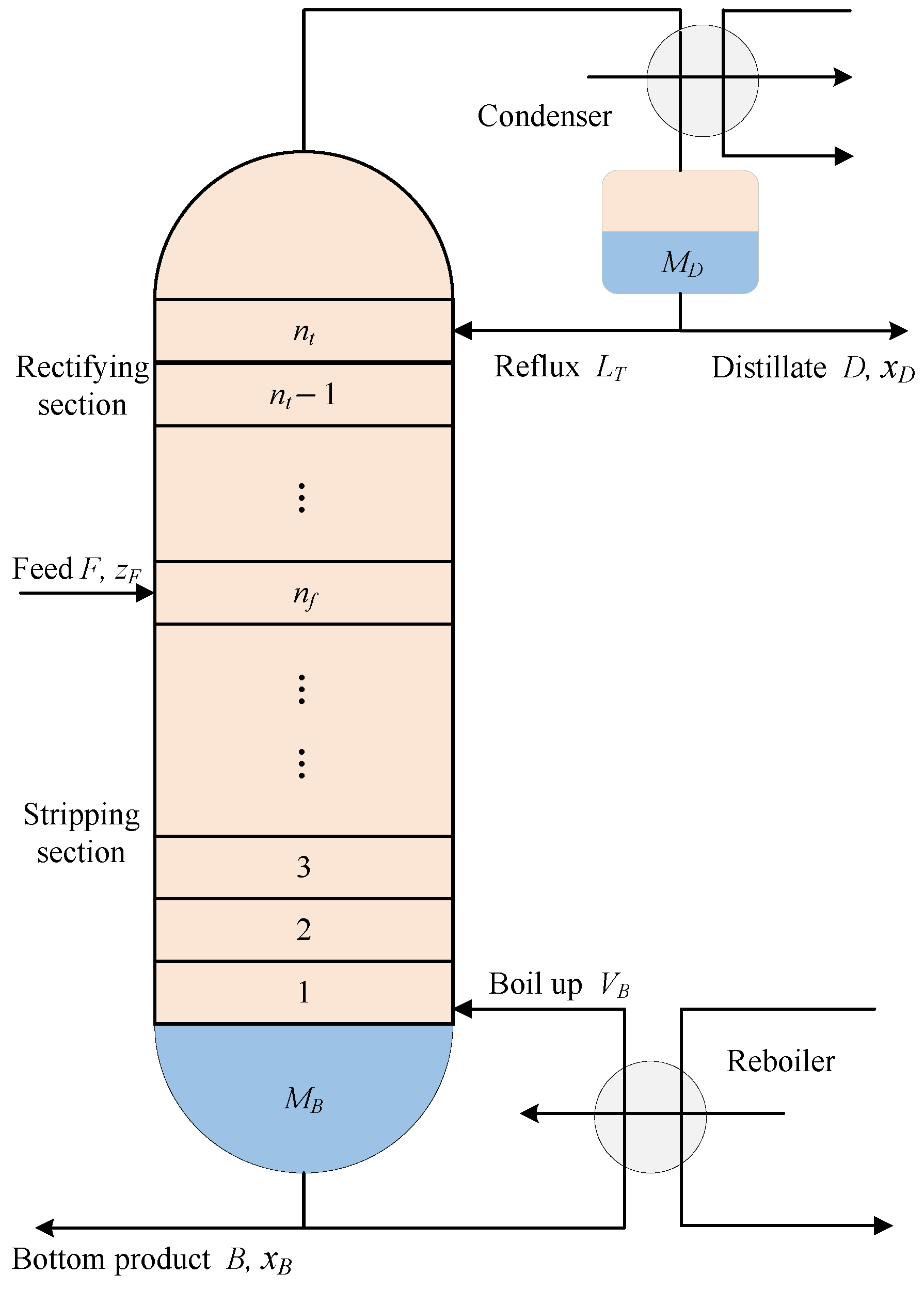
The high-purity distillation column capitalizes on the fact that each component within the feed mixture exhibits distinct volatility characteristics. Specifically, the vapor pressure of each component differs at a given temperature. This process facilitates the transfer of a light-boiling component from the liquid phase to the gas phase and a heavy-boiling component from the gaseous phase into the fluid phase, thereby attaining the objective of separation [22], as depicted in Figure 1.
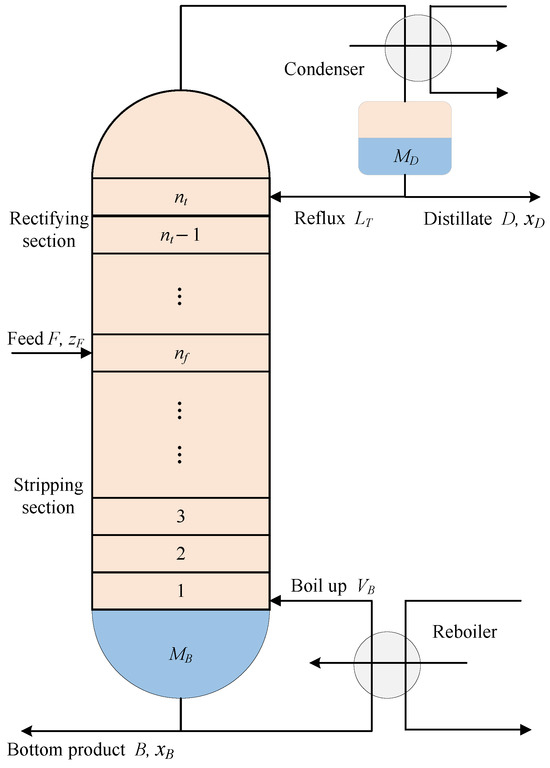
Figure 1.
Two-product distillation column structure.
The process model of the distillation column is composed of 41 stages. The bottom tray is a reboiler, and the top tray is a condenser. Table 1 summarizes the nomenclature of each process parameter and the nominal values employed in this distillation column model. The subsequent section shows the nonlinear models of every component inside the high-purity distillation column:

Table 1.
The parameters involved in the high-purity distillation column’s process.
Reboiler:
where and . Meanwhile, is the gas–fluid balance equation, and its mathematical expression is presented in detail later.
Condenser:
where .
Feed tray:
Other distillation trays:
where .
Gas–fluid balance equation:
Fluid flow equation:
Gas flow velocity equation:
where i represents the layer number concerned.
3. The Dual-Loop MADRC Scheme for the Column
The dual-loop MADRC scheme entails designing two controllers of MADRC through the adjustment of and to, respectively, control the compositions of and , as depicted in Figure 2. To ensure the stability of the distillation column, the LV configuration [23] is adopted. Additionally, two proportional-integral (PI) controllers are designed: one enables D to govern , and the other allows B to manage . The parameters of the two PI controllers for the and are and , respectively. Note that other advanced strategies like ADRC are also applicable.
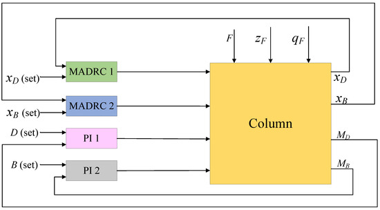
Figure 2.
The dual-loop MADRC scheme for the distillation column.
3.1. The Regular Design of Linear ADRC
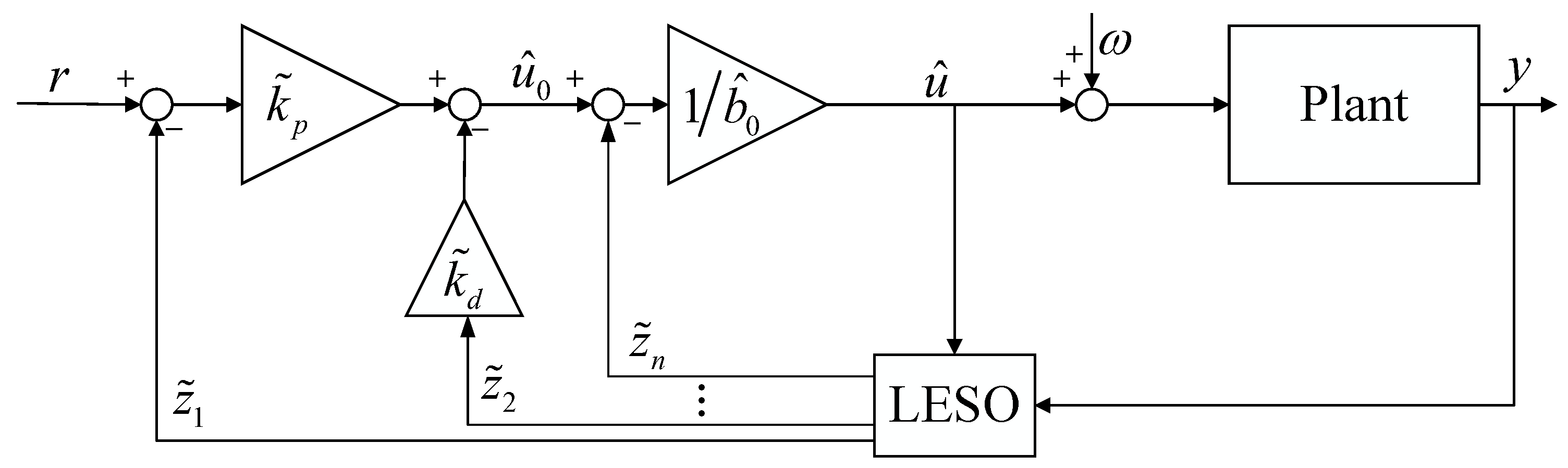
The concept of the frequency scale is employed in the linear ADRC controller. The nonlinear links within the nonlinear ADRC controller are simplified, and the linear structures are integrated [13]. This integration enables the establishment of a relationship between the parameters associated with the controller’s bandwidth and those of the observer. As a result, the number of parameters is decreased from nine to three. This reduction not only diminishes the complexity and debugging intricacy of the system but also enhances the practicality and reliability, as displayed in Figure 3.
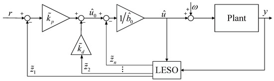
Figure 3.
The structure of the n-order LADRC.
A common nth-order model can be described as
where , , , , and denote the output, the control signal, external disturbances, the comprehensive function, and the input gain of the system, respectively.
Define the total disturbance as
where f is differentiable, and is the estimation of . By selecting the state variables , the state equation of Equation (9) can be obtained as
where . Thus, the state equation of linear ESO is able to be constructed as
where are the parameters of linear ESO. Relying on the bandwidth-parameterization approach [13], the succeeding conclusions can be obtained as
where is the observer bandwidth. Therefore, it is possible to configure the characteristic equation of the ESO as
The above configuration places the poles of Equation (14) at the same position , which not only guarantees the system’s stability but also offers a superior transition process.
The state-feedback control law (SFCL) is specified as
By ignoring the estimation error of with respect to the total disturbance f, the initial model is capable of being approximated as a series of integrals structure from
The approximate system in Equation (16) is able to be readily governed by applying a PD controller
where r is the reference input of the system and is the th-order derivative of r. and serve as the gain parameters of the controller.
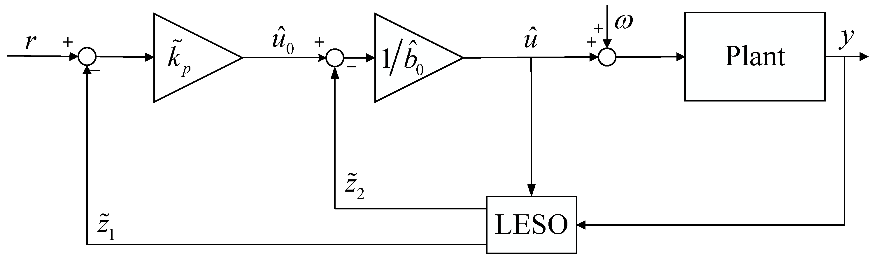
Based on the above analysis, a first-order ADRC can be designed as shown in Figure 4 if the system is of the following form:
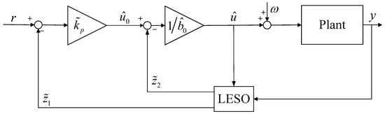
Figure 4.
The structure of the first-order LADRC.
Define the total disturbance as
Then, are selected as state variables, and according to Equation (11), one can obtain
Thus, the ESO of Equation (18) is able to be constructed as
According to the bandwidth-parameterization method, the following conclusion can be obtained:
And the SFCL is specified as
According to Equation (17), one can have
where is the gain of the SFCL.
3.2. The Design of MADRC for and
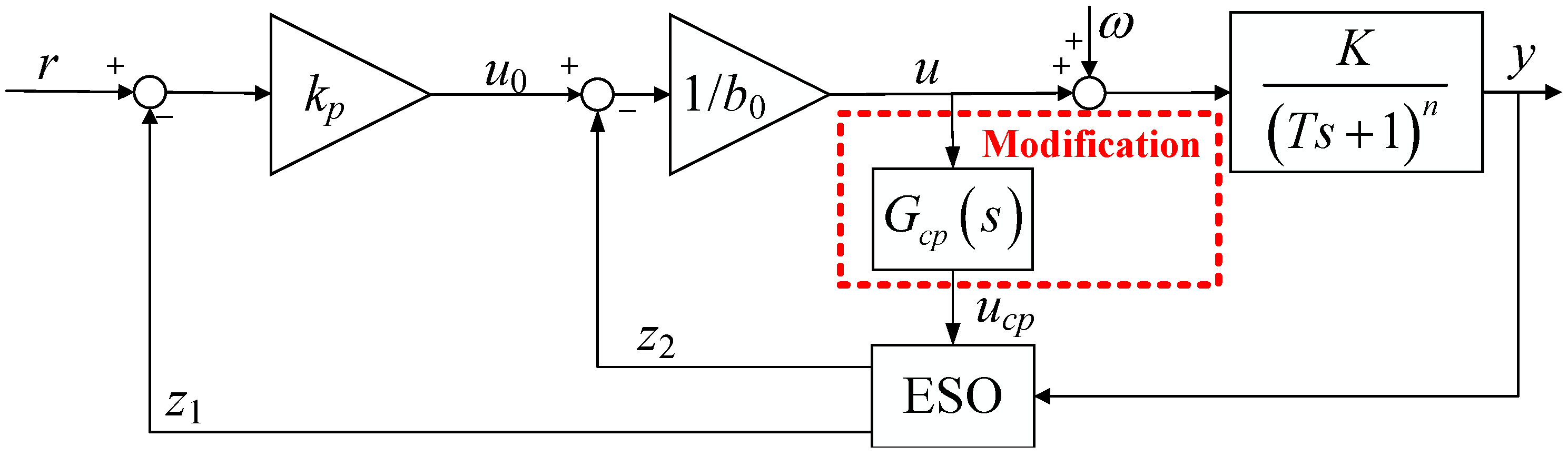
In this section, a MADRC based on ADRC is proposed by adding a compensation part, as shown in Figure 5. A typical high-order inertia system is defined as
where K, T, and are the system gain, time constant, and system order, respectively.
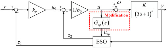
Figure 5.
The structure of the first-order linear ADRC.
The compensation part of MADRC is presented in the red box in Figure 5. In this context, the control signal u passes through the compensation part prior to reaching the ESO. The compensation part, which is chosen in accordance with Equation (26), is presented as
The inherent dynamic characteristics of the high-order inertia system give rise to a time lag in the output. Subsequently, synchronizes u with y before they enter the ESO, thus enabling the ESO to provide a more accurate estimate of the state of the system in Equation (26).
In this scenario, the ESO shares a similar structure to that of the regular linear ADRC. However, the control signal is substituted with the output of , denoted as . Thus, the ESO of Equation (26) is able to be constructed as
where is utilized to signify the approximation of the input gain parameter. When the parameters of the ESO are suitably tuned, the output can track and compensate f well through the SFCL, that is
and
where is the gain of the SFCL.
It should be noted that MADRC can make use of the bandwidth-parameterization approach. Based on this, the subsequent conclusion is derived:
Evidently, there are no extra parameters within MADRC that need tuning. MADRC adopts the advantages of ADRC, such as a simple structure and easy implementation.
According to Equation (1), the following form can be obtained as
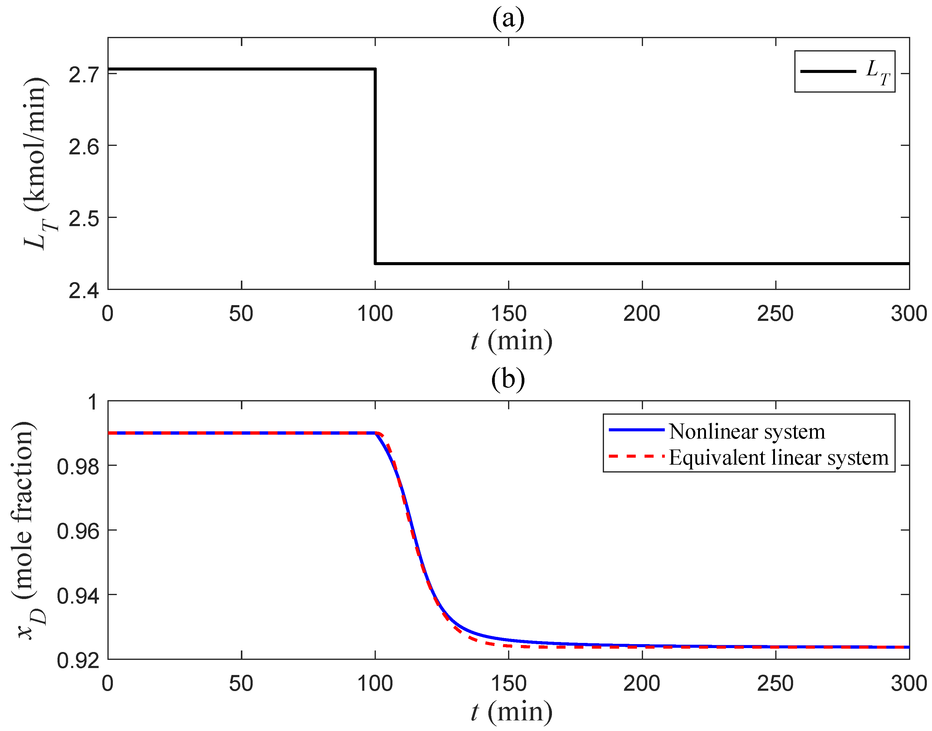
where is directly controlled by . In the proximity of stable operation conditions of the distillation column, at min, with kept constant, a step change of times the initial value is applied to . Dynamic data of are collected. For the loop with as the input and as the output, denoted as the loop , a fitting technique is employed to establish a high-order inertial linear model for characterizing its dynamic behavior. The detailed fitting effect is shown in Figure 6. Subsequently, the loop is obtained as
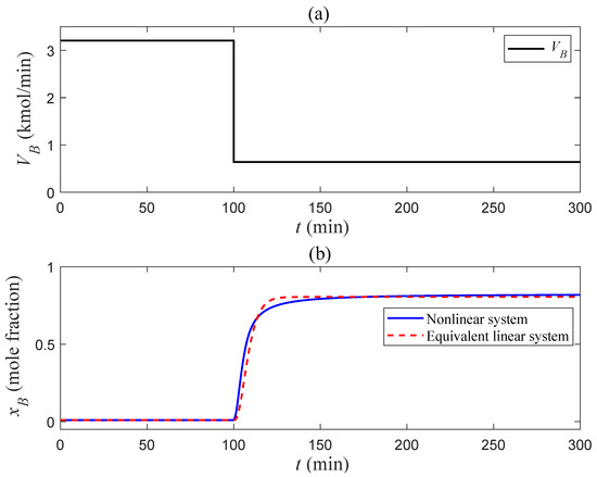
Figure 6.
The comparison of the output of the nonlinear system and that of an equivalent linear system for the loop . ((a): The step-change graph of versus time, (b): The outputs between nonlinear and equivalent linear systems over time).
It is evident that the model boasts sufficient accuracy and is well suited for the design of the compensation part . Then, the mathematical expression of is
For Equation (33), the ESO is able to be constructed as
Then, the SFCL is selected as
and
Likewise, in the proximity of stable operation conditions of the distillation column, at min, with kept constant, a step change of times the initial value is applied to . Dynamic data of are collected. For the loop with as the input and as the output, denoted as the loop , a fitting technique is employed to establish a high-order inertial linear model for characterizing its dynamic behavior. The detailed fitting effect is shown in Figure 7. Subsequently, the loop is obtained as
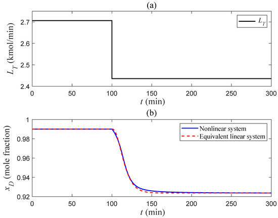
Figure 7.
The comparison of the output of the nonlinear system and that of an equivalent linear system for the loop . ((a): The step-change graph of versus time, (b): The outputs between nonlinear and equivalent linear systems over time).
It is evident that the model boasts sufficient accuracy and is well suited for the design of the compensation part . Then, the mathematical expression of is
The design of the ESO and the control law is the same as above.
Note that in this section, the nonlinear distillation column model is approximated as linear models in Equations (33) and (38) specifically to design the linear compensation parts in Equations (34) and (39) for the dual-loop MADRC scheme. It is crucial to emphasize that although this approximation is made for design purposes, all simulation experiments of the four control schemes presented in this paper are rigorously conducted for the original nonlinear distillation column model, as described in Section 2.
3.3. Stability Analysis of MADRC
In this subsection, the stability analysis of MADRC is conducted. According to Section 3.2, the state-space representation of the ESO of MADRC can be written as
where , , , and .
In this paper, is defined as the feedback control error, and is defined as the ESO’s state estimation error [19]. Suppose the value of the reference input r remains unchanged, that is, . Then, the closed-loop dynamic error equation of MADRC can be written as
where , , , , , , and is the differential of the total disturbance f.
As can be observed from Equation (41), given that the observer bandwidth is typically several times that of the feedback control bandwidth , the error dynamics can be divided into two components: of the ESO with a relatively fast response, and with a relatively sluggish response property. This system with error dynamics featuring both rapid and sluggish components is a typical characteristic of singular perturbation systems. As a result, in this paper, the utilization of singular perturbation theory is considered to demonstrate the stability of MADRC.
To convert Equation (41) into the standard singular perturbation model, let the state estimation error of the ESO and the singular parameter be selected as , so the error dynamics of MADRC can be finally written as
where , .
As per the singular perturbation theory, the standard singular perturbation model is
where and .
By setting the singular parameter to zero, one can determine the quasi-steady-state solutions and pertaining to the system.
The specific solutions p and q can be represented via the two-time-scale asymptotic expansions. Here, the quasi-steady components and are formulated in the t-scale, while the transient elements and are specified in the -scale.
where is known as the boundary-layer subsystem, whose dynamic characteristic is
Then, the key theorem from [19] in the domain of singular perturbation theory is presented.
Assumption 1.
The balance of the boundary-layer subsystem is uniformly asymptotically stable with respect to and , and the quantity lies within its region of attraction.
Assumption 2.
For , along the trajectories of and , the real parts of the eigenvalues of are less than a fixed negative constant. That is, .
Theorem 1.
Provided that Assumption 1 and Assumption 2 hold, . Then, for all , the approximations and hold true. Additionally, there exists a time , such that .
Proof of Theorem 1.
Then, this paper examines whether the closed-loop error dynamic equation of MADRC meets the above two assumptions, aiming to prove the stability of MADRC. The closed-loop error dynamic system in Equation (42) is written in the form of Equation (43) as
where and .
Consequently, the quasi-steady-state solutions are
Besides, the boundary-layer subsystem exists as
The balance points of the boundary-layer subsystem are , and the balance points are uniformly asymptotically stable. Suppose that the initial tracking error of the ESO is 0, i.e., , so lies within the attraction domain of the balance points. Assumption 1 holds true.
For the singular parameter , along and , . Thereafter, the eigenvalues of are calculable from
So, . Assumption 2 holds true.
According to Theorem 1, and hold true in the time range . And because of , is true in . For , since , is uniformly asymptotically stable, that is, , so .
In summary, when the value of is relatively large and the singular parameter is a small positive number, then there are bandwidth parameters and , making Equation (42) controlled by MADRC uniformly asymptotically stable. □
4. The Tuning Rule of the Dual-Loop MADRC Scheme
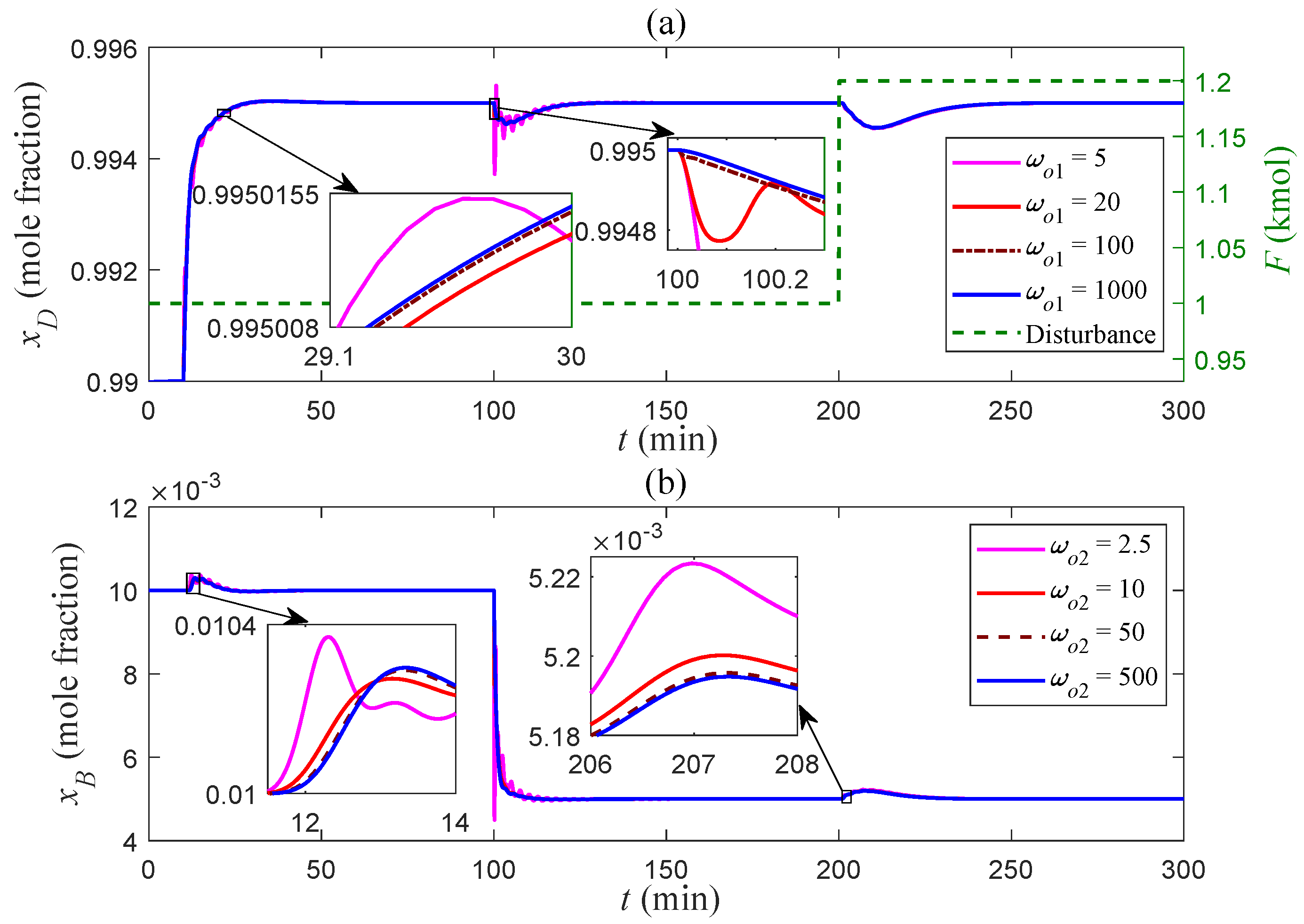
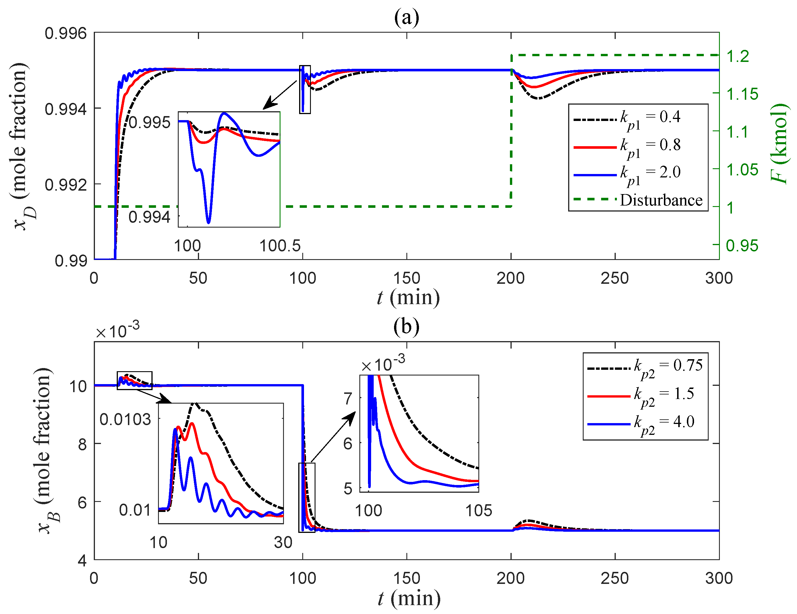
Considering the structural disparities between the dual-loop MADRC scheme and the regular ADRC, the parameters of the former exert different influences on control performance. Accordingly, the parameter tuning for the dual-loop MADRC scheme presents its own set of specific features. To determine the optimal parameters’ range of the dual-loop MADRC scheme, the single-variable method is utilized to explore the behavior of control performance with various MADRC parameter settings. Note that the reference input of increases from to at min. At min, the reference input of decreases from to at min. And the disturbance is configured as follows: F is increased from 1 kmol/min to kmol/min at min. The outcomes concerning the controlling effectiveness under diverse values of , and are illustrated within Figure 8, Figure 9 and Figure 10, respectively.
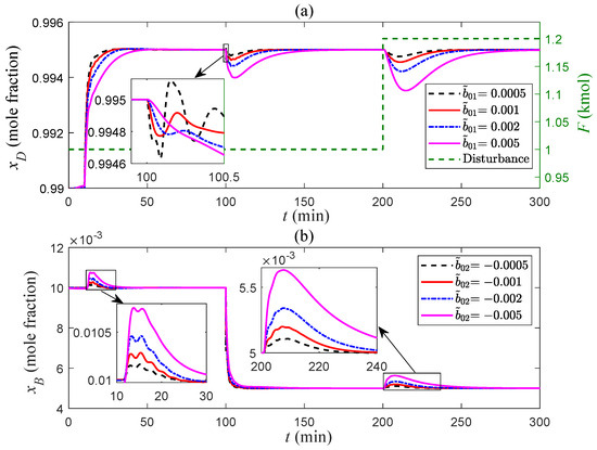
Figure 8.
The outputs and with different . ((a): The outputs and disturbance F, (b): The outputs ).
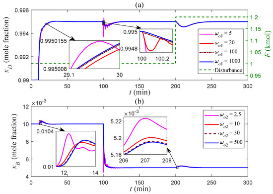
Figure 9.
The outputs and with different . ((a): The outputs and disturbance F, (b): The outputs ).
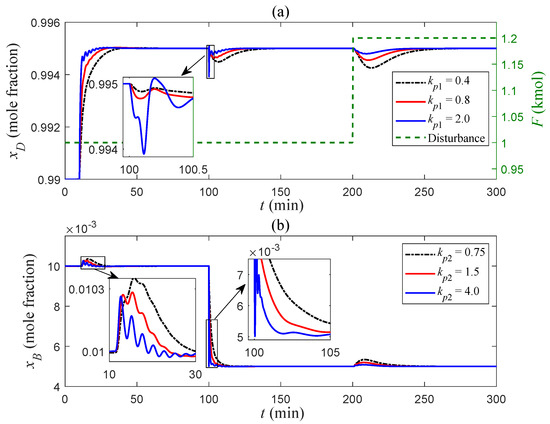
Figure 10.
The outputs and with different . ((a): The outputs and disturbance F, (b): The outputs ).
As depicted in Figure 8, when the value of is relatively low, it brings about a more powerful control force, but the fluctuations become more prominent. On the contrary, a relatively high value of causes a weaker control force and less intense fluctuations. By extensive simulation experiments, the optimal range of parameter in the loop is determined to be , and the optimal range of parameter in the loop is . Additionally, an inverse relationship between the values of and is observed, meaning their absolute values are equal while their signs are opposite.
As shown in Figure 9, when is small, the outputs of the loop and exhibit substantial fluctuations. Conversely, when is sufficiently large, the outputs exhibit negligible alterations. Given that a larger enhances the susceptibility to measurement noise and increases the computational stress upon the ESO, the value of needs to be adjusted to an appropriate value that ensures minimal output variation. Through extensive simulation experiments, the optimal range of parameter in the loop is determined as , and the optimal range of parameter in the loop is determined as . Moreover, it turns out that .
From Figure 10, when is relatively large, the loop and the loop show better disturbance rejection capabilities. However, the system output experiences more severe oscillations when tracking changes in the input signal. After a lot of simulation experiments, the optimal range of parameter in the loop is determined as , and the optimal range of parameter in the loop is determined as .
5. Simulation and Experiment Validation
5.1. Simulation Validations
The following analysis focuses on comparing the control performance of four control schemes under three operating conditions (A, B, and C): the dual-loop MADRC, cascade PID control (CPID), regular ADRC (ADRC), and PID control (PID). Among them, MADRC is tuned according to Section 4. ADRC is tuned by [13]. The parameters of CPID can be found in [11]. The parameters of PID are tuned via the trial-and-error method, adhering to these three principles: (1) With no overshoot or an overshoot less than , the outputs and of the distillation column should respond as swiftly as possible. (2) The outputs and should remain free from significant oscillations. (3) PID controller parameters must exhibit adequate robustness across various operating conditions to ensure consistent control performance of the distillation column. Each controller’s tuned parameters are presented in Table 2 and Table 3. Note that the parameters of the four control schemes are fixed parameters and do not change with the variation in operating conditions.
Table 2.
The tuned parameters of four control schemes for the loop .
Table 3.
The tuned parameters of four control schemes for the loop .
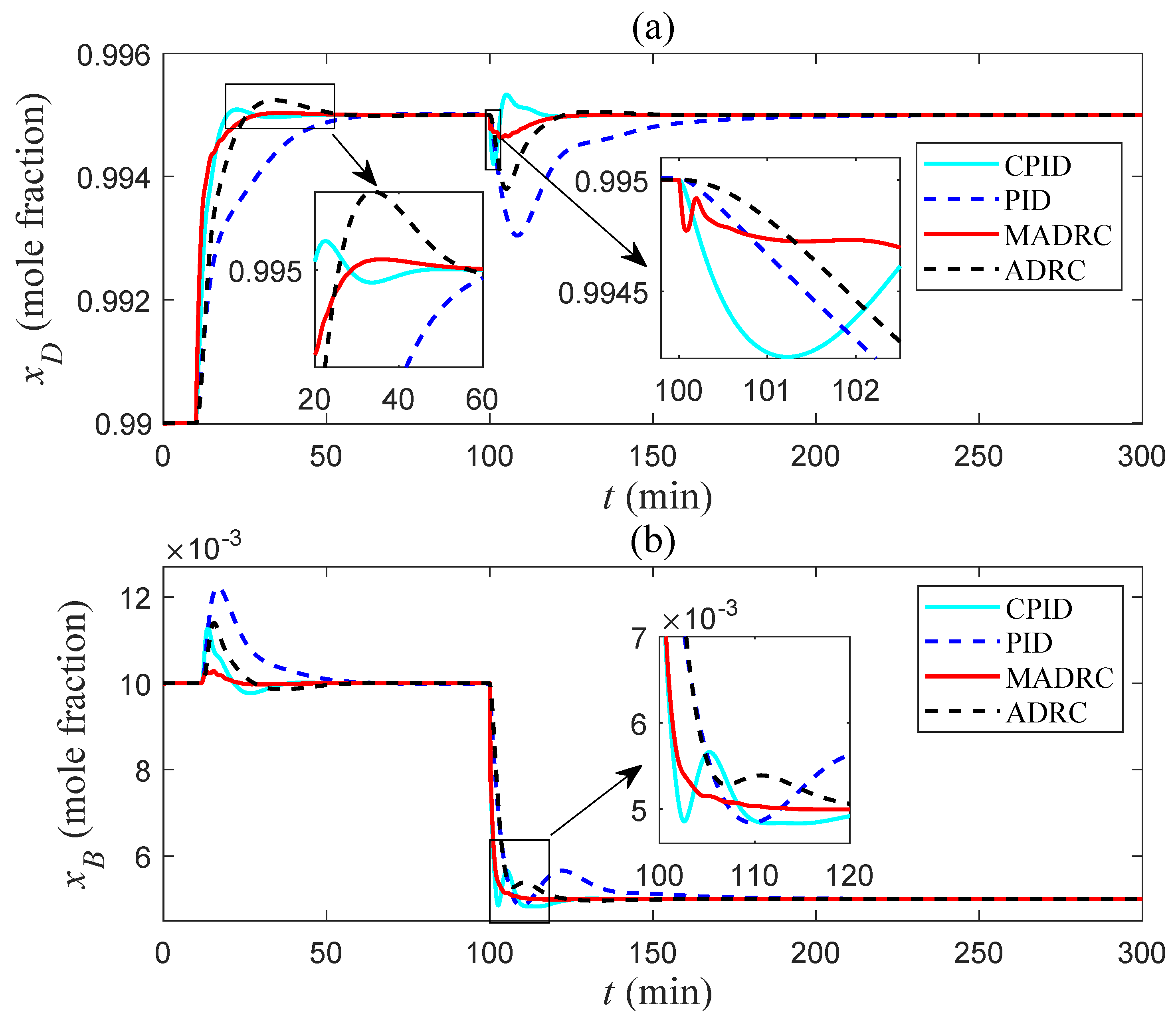
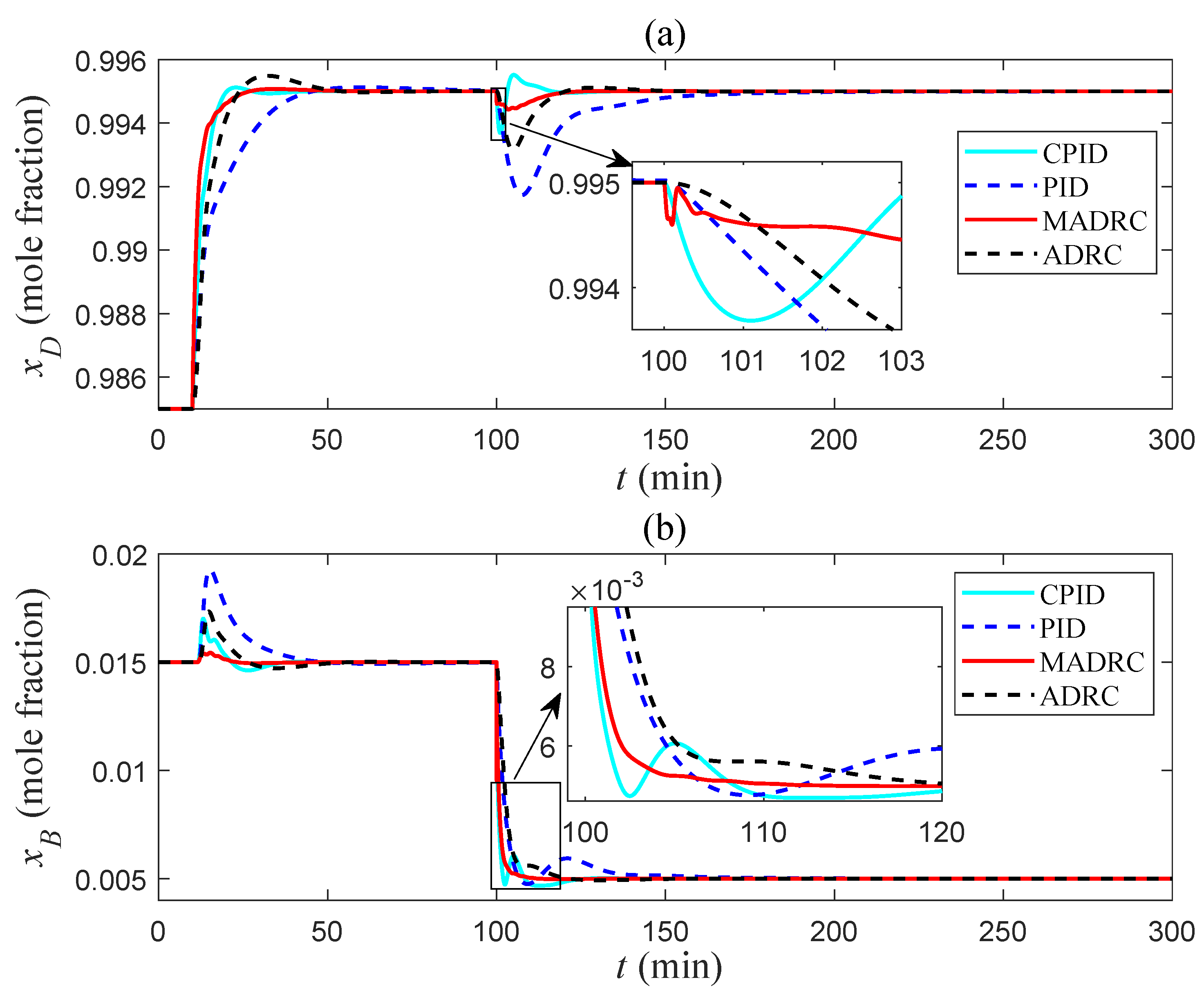
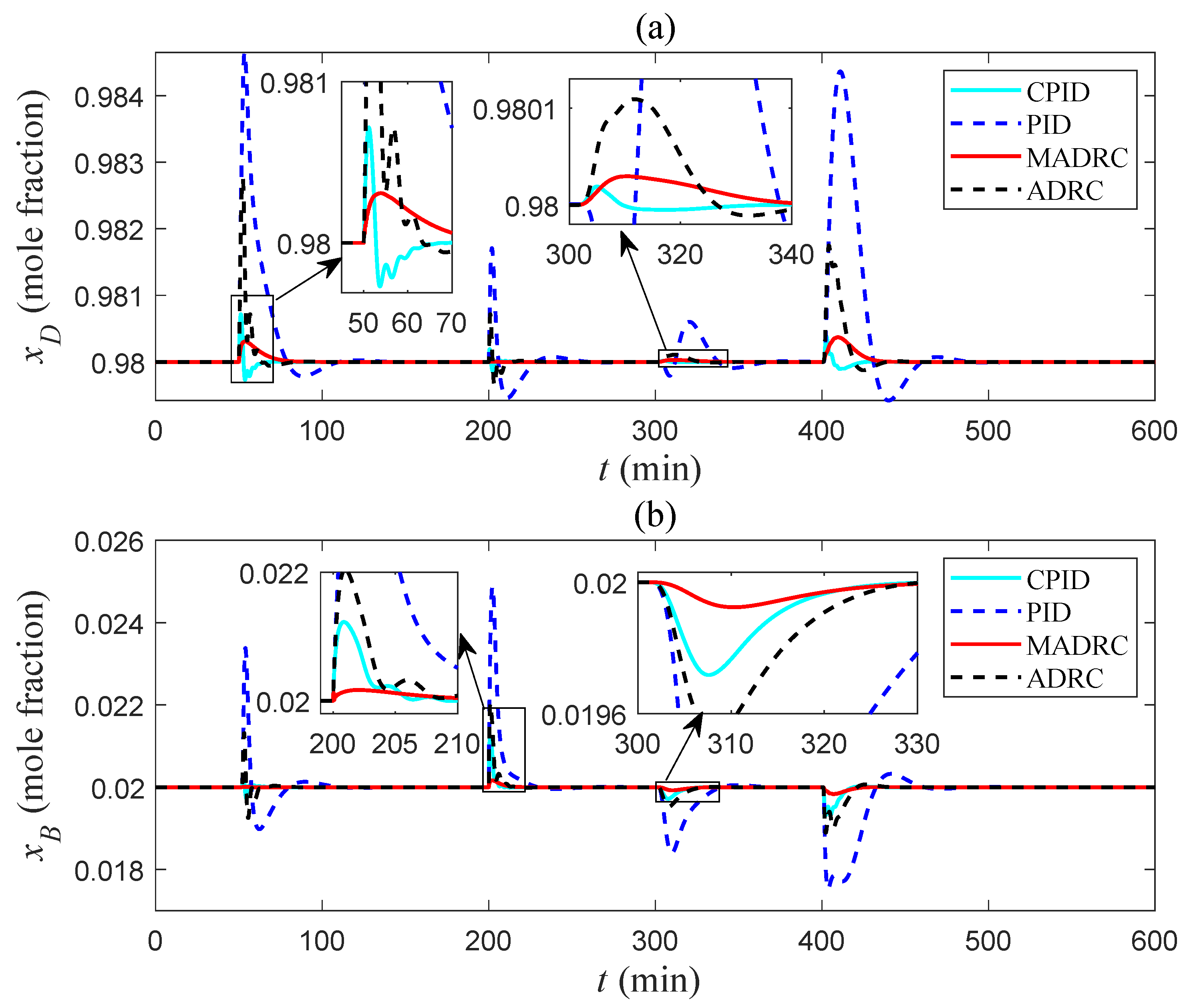
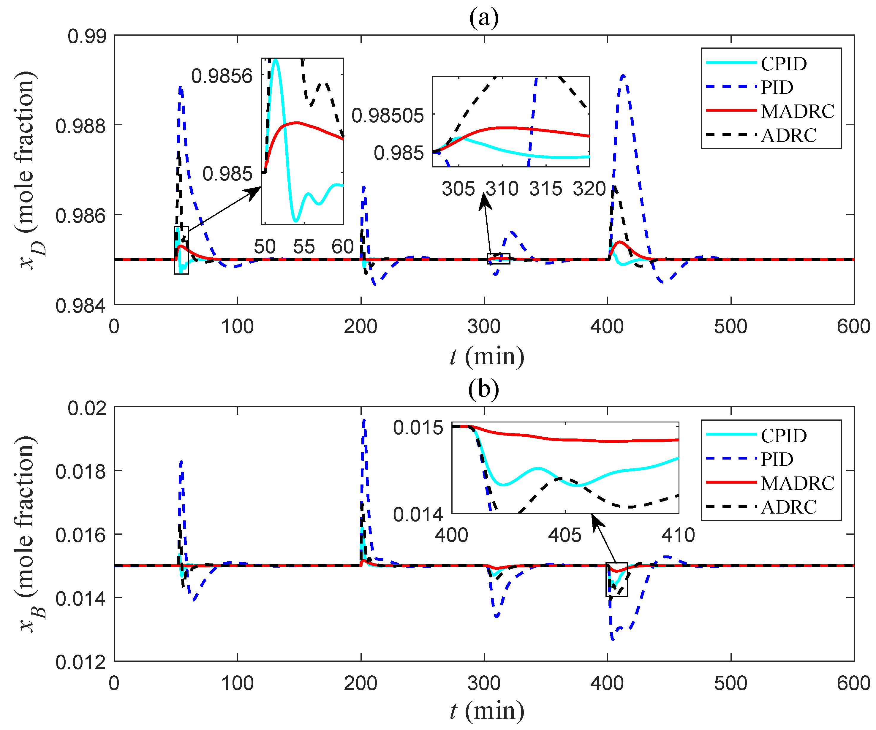
Firstly, the tracking performance of the four control schemes under the three operating conditions is compared. Operating condition A: the reference input of increases from to at min, while the reference input of decreases from to at min. Operating condition B: the reference input of increases from to at min, while the reference input of decreases from to at min. Operating condition C: the reference input of increases from to at min, while the reference input of decreases from to at min. The comparison results of four control schemes are set forth in Figure 11, Figure 12 and Figure 13.

Figure 11.
The tracking performance of four control schemes under operating condition A. ((a): The outputs , (b): The outputs ).
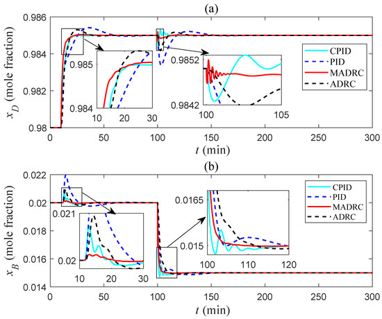
Figure 12.
The tracking performance of four control schemes under operating condition B. ((a): The outputs , (b): The outputs ).
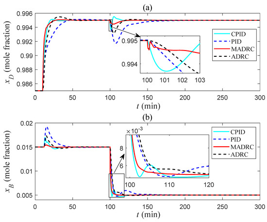
Figure 13.
The tracking performance of four control schemes under operating condition C. ((a): The outputs , (b): The outputs ).
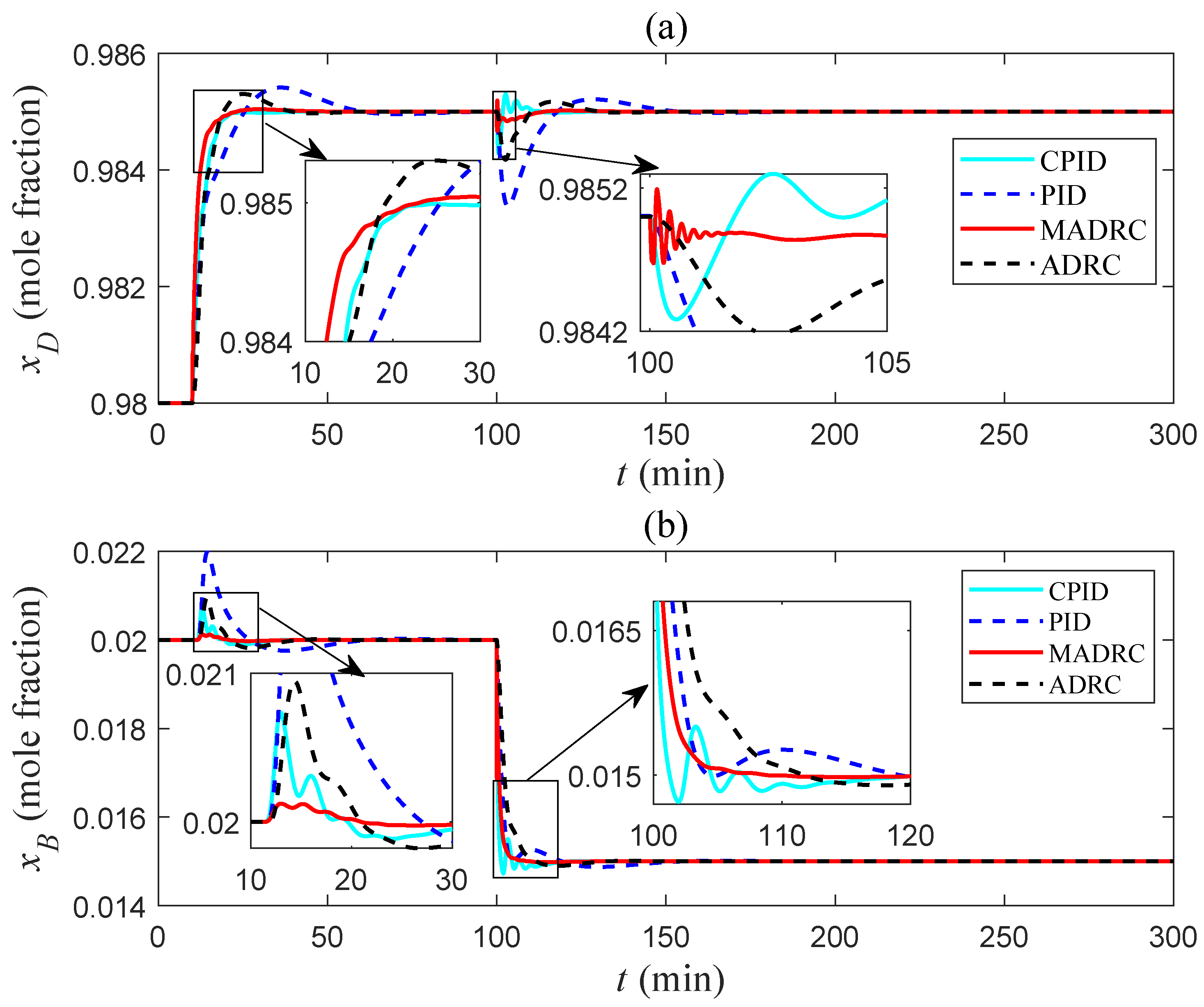
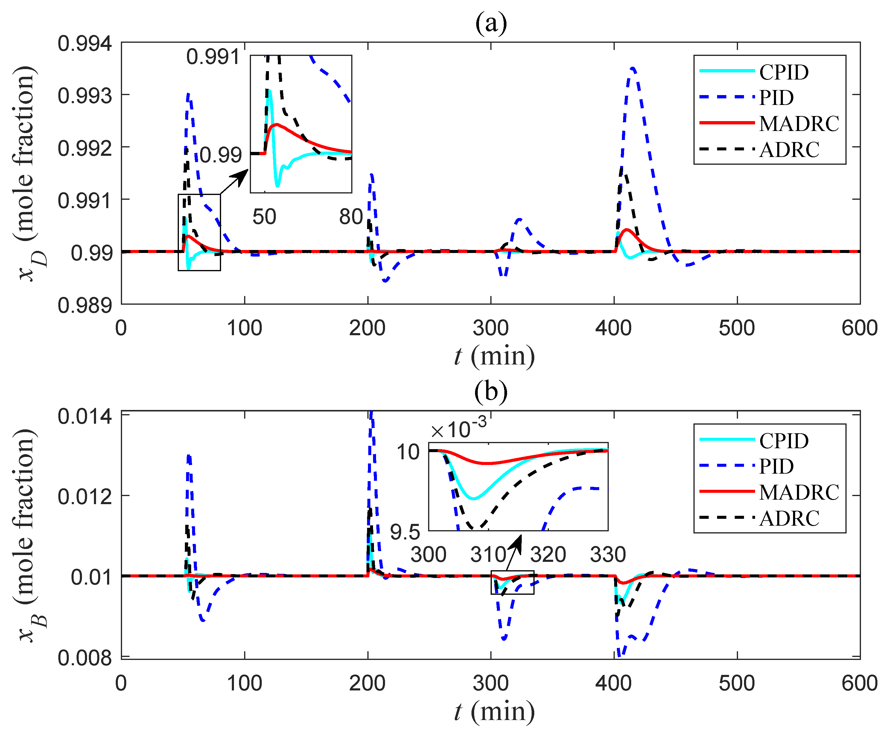
Subsequently, the disturbance rejection performance (external disturbances and model uncertainties) of four control schemes under three operating conditions is compared. Operating condition A: the reference input of is , while the reference input of is . Operating condition B: the reference input of is , while the reference input of is . Operating condition C: the reference input of is , while the reference input of is . The following are the settings for external disturbances and model uncertainties. Specifically, at min, a step disturbance with amplitude is imposed on , and at min, another with amplitude is applied to . Model uncertainty is considered to arise from the divergence between the process-related models and the controller models, which is caused by the perturbation of system parameters. The changes in system parameters are: at min, rises from to and F grows from 1 kmol/min to kmol/min at min. The control performance of the control schemes is depicted in Figure 14, Figure 15 and Figure 16.
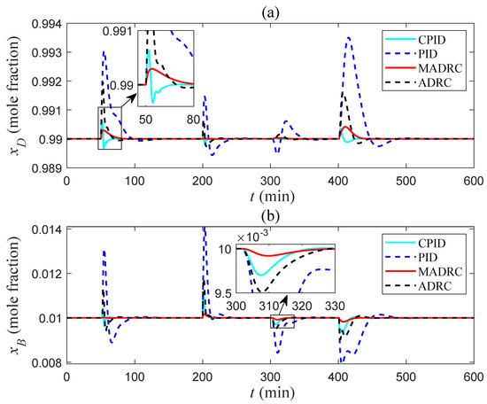
Figure 14.
The disturbance rejection performance of four control schemes under operating condition A. ((a): The outputs , (b): The outputs ).
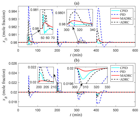
Figure 15.
The disturbance rejection performance of four control schemes under operating condition B. ((a): The outputs , (b): The outputs ).
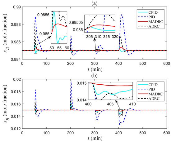
Figure 16.
The disturbance rejection performance of four control schemes under operating condition C. ((a): The outputs , (b): The outputs ).
5.2. Discussions
As can be seen from Figure 11, Figure 12 and Figure 13, the dual-loop MADRC scheme attains the fastest equilibrium state, the minimum overshoot, and the smallest fluctuation amplitude of and under all three working conditions, demonstrating the most excellent tracking performance. Compared with the dual-loop MADRC scheme, the CPID control scheme also demonstrates a relatively high response speed, but there is always a large oscillation when tracks the reference input. In contrast, the PID control scheme displays the slowest response speed, the poorest tracking efficacy, and the maximum overshoot.
From Figure 14, Figure 15 and Figure 16, it can be seen that the dual-loop MADRC scheme exhibits the optimal disturbance rejection performance under all three operating conditions. The ESO and the compensation part within this scheme can estimate model uncertainties and external disturbances instantaneously and implement compensations. Consequently, the dual-loop MADRC scheme demonstrates the ability to counteract model uncertainties and external disturbances.
To make the advantages of the dual-loop MADRC scheme more prominent, the integral absolute error (IAE) indexes of four control schemes under three operating conditions are calculated. These IAE indexes are presented in Figure 11, Figure 12, Figure 13, Figure 14, Figure 15 and Figure 16. Among them, is an index of tracking performance, is an index of anti-interference performance, and is a comprehensive performance index of the sum of and . As can be seen from Table 4, Table 5 and Table 6, the of the dual-loop MADRC scheme is the smallest, indicating it has the best comprehensive control performance.
Table 4.
IAE indexes of four control schemes under operating condition A.
Table 5.
IAE indexes of four control schemes under operating condition B.
Table 6.
IAE indexes of four control schemes under operating condition C.
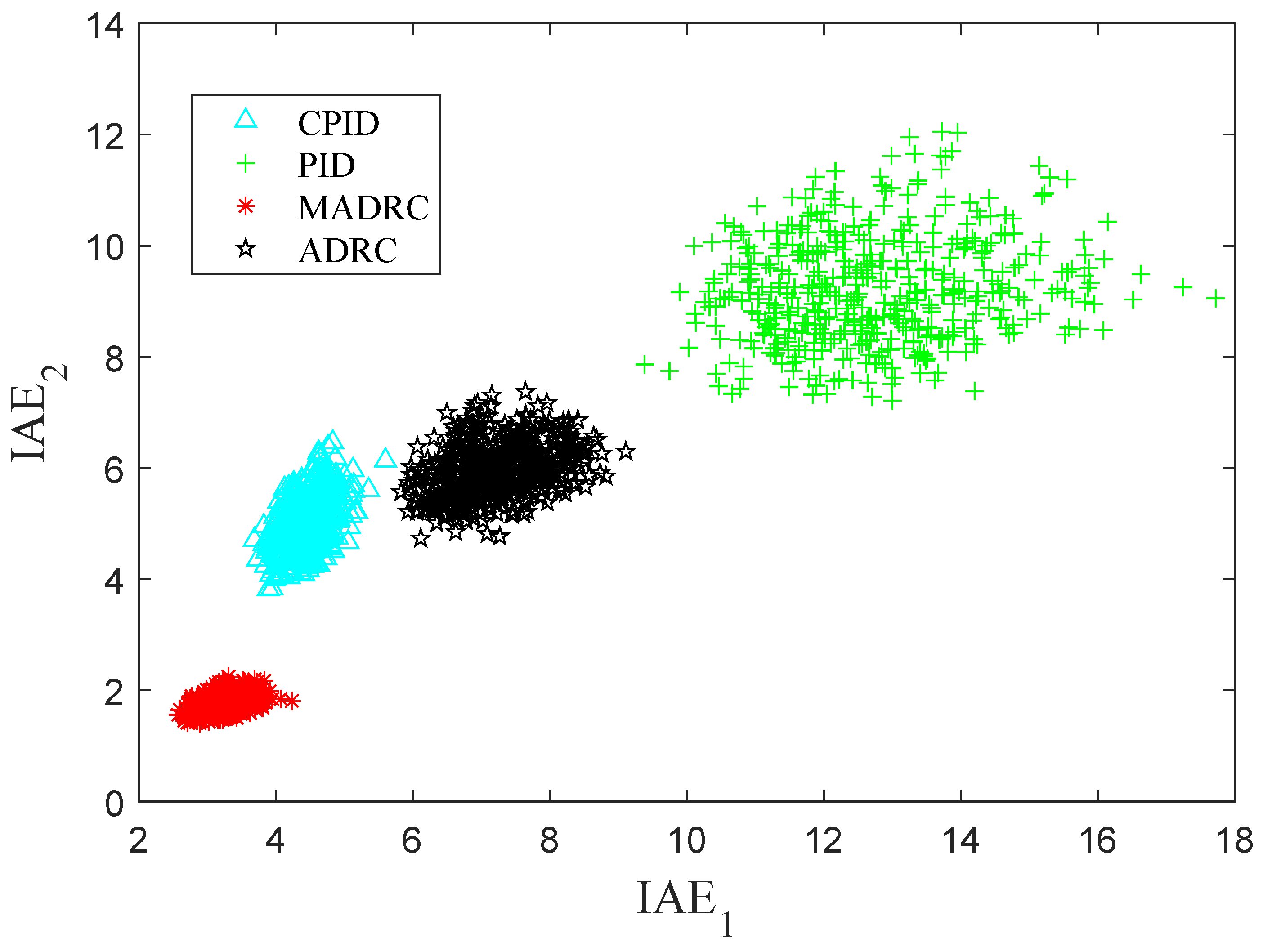
The Monte Carlo method, grounded in the law of large numbers, conducts repeated simulations by generating sequences of random numbers [24]. It transforms complex systems into stochastic process modeling and numerical computations, effectively reducing the complexity of research. For a more in-depth evaluation of the four control schemes’ robustness, this paper introduces Monte Carlo trials. Keeping the controller parameters unaltered, random perturbations of around the nominal values are applied to the original values of and , respectively. Additionally, random perturbations at of their nominal values are performed on the relative volatility and time constant . Moreover, there is a gain uncertainty that varies within for each input channel. The disturbances and uncertainties configured in the Monte Carlo trials are meticulously designed to faithfully reproduce real operational scenarios. Note that the reference input of increases from to at min. At min, the reference input of decreases from to at min. The integral absolute error (IAE) indexes of four control schemes are collected from the start time to 300 min for each simulation. functions as the evaluation index for the performance of the loop , and the performance of the loop is measured by . Monte Carlo trials will be carried out randomly 800 times. The distribution of the IAE indexes for four control schemes is depicted in Figure 17. Among them, the smaller the IAE indexes are, the better the tracking and disturbance rejection capabilities will be, and the denser the distribution of the IAE indexes is, the better the performance robustness will be [18]. As clearly depicted in Figure 17, the dual-loop MADRC scheme exhibits the most concentrated distribution and the minimum values of the IAE indexes. Consequently, the dual-loop MADRC scheme can effectively maintain optimal control performance in the face of system uncertainties, thereby indicating strong application potential.

Figure 17.
The distributions of IAE with uncertain models.
6. Conclusions
ADRC has been extensively utilized in diverse control systems. However, the performance of ADRC is suboptimal when it comes to dealing with systems characterized by significant time delays, such as high-purity distillation columns. To address this issue, this paper devises a dual-loop MADRC scheme and applies the MADRC algorithm to a high-purity distillation column. MADRC inherits the merits of ADRC and can handle the delay problem more proficiently by incorporating a compensation part. In the compensation part, the control signal is synchronized with the output of the high-purity distillation column before entering the ESO, thereby enabling the ESO to estimate the state more precisely. Furthermore, this paper utilizes singular perturbation theory to demonstrate the stability of MADRC. The control performance of the dual-loop MADRC scheme is contrasted against that of a cascade PID control scheme, a regular ADRC scheme, and a PID control scheme. The simulation results indicate that the dual-loop MADRC scheme proposed in this paper can effectively track the reference and exhibits superior disturbance rejection performance. Moreover, this is verified through Monte Carlo trials. In future research, interactions between MADRC and higher-level advanced process control techniques (such as MPC and nonlinear MPC) or real-time optimization (RTO) schemes will be investigated.
Author Contributions
Conceptualization, X.S. and Z.L.; methodology, Y.Z. and Z.W.; software, Z.L.; validation, X.S., Y.Z., and Z.W.; formal analysis, J.S.; investigation, J.S.; resources, J.Z.; data curation, Z.W.; writing—original draft preparation, Z.W., Z.L., and J.G.; writing—review and editing, Z.L.; visualization, Z.W.; supervision, X.S.; project administration, X.S. and Z.L.; funding acquisition, X.S. and Y.Z. All authors have read and agreed to the published version of the manuscript.
Funding
The authors declare that this study received funding from Anhui Province Science and Technology Breakthrough Plan Project (Key Project) under grant No. 202423110050043.
Data Availability Statement
All the data have been used with confidence.
Conflicts of Interest
Author Xudong Song, Yuedong Zhao, and Jingzhong Guo were employed by the company Anhui CasWinners Digital Technology Co., Ltd. Jian Zhang was employed by the company Anhui Wanwei Group Co., Ltd. The remaining authors declare that the research was conducted in the absence of any commercial or financial relationships that could be construed as potential conflicts of interest.
References
- Yuan, Y.; Huang, K.; Qian, X.; Chen, H.; Zang, L.; Zhang, L. Enhanced temperature difference control of distillation columns based on the averaged absolute variation magnitude. Chin. J. Chem. Eng. 2021, 29, 266–278. [Google Scholar] [CrossRef]
- Torres Cantero, C.A.; Pérez Zúñiga, R.; Martínez García, M.; Ramos Cabral, S.; Calixto-Rodriguez, M.; Valdez Martínez, J.S.; Mena Enriquez, M.G.; Pérez Estrada, A.J.; Ortiz Torres, G.; Sorcia Vázquez, F.d.J.; et al. Design and Control Applied to an Extractive Distillation Column with Salt for the Production of Bioethanol. Processes 2022, 10, 1792. [Google Scholar] [CrossRef]
- Zhu, Y.; Liu, X. Dynamics and control of high purity heat integrated distillation columns. Ind. Eng. Chem. Res. 2005, 44, 8806–8814. [Google Scholar] [CrossRef]
- Fu, Y.; Liu, X. Nonlinear dynamic behaviors and control based on simulation of high-purity heat integrated air separation column. ISA Trans. 2015, 55, 145–153. [Google Scholar] [CrossRef]
- Karan, S.; Dey, C.; Mukherjee, S. Simple internal model control based modified Smith predictor for integrating time delayed processes with real-time verification. ISA Trans. 2022, 121, 240–257. [Google Scholar] [CrossRef]
- Tahir, N.M.; Zhang, J.; Armstrong, M. Control of heat-integrated distillation columns: Review, trends, and challenges for future research. Processes 2024, 13, 17. [Google Scholar] [CrossRef]
- Shi, X.; Zhao, H.; Fan, Z. Parameter optimization of nonlinear PID controller using RBF neural network for continuous stirred tank reactor. Meas. Control 2023, 56, 1835–1843. [Google Scholar] [CrossRef]
- Skogestad, S. Simple analytic rules for model reduction and PID controller tuning. J. Process Control 2003, 13, 291–309. [Google Scholar] [CrossRef]
- Zangina, J.A.S.; Wang, W.; Qin, W.; Gui, W.; Zhang, Z.; Xu, S.; Liu, X. Model predictive control of a high-purity internal thermally coupled distillation column. Chem. Eng. Technol. 2021, 44, 1294–1301. [Google Scholar] [CrossRef]
- Ping, Z.; Li, Y.; Huang, Y.; Lu, J.G.; Wang, H. Global robust output regulation of a class of MIMO nonlinear systems by nonlinear internal model control. Int. J. Robust Nonlinear Control 2021, 31, 4037–4051. [Google Scholar] [CrossRef]
- Cheng, Y.; Gao, Z.; Sun, M.; Sun, Q. Cascade active disturbance rejection control of a high-purity distillation column with measurement noise. Ind. Eng. Chem. Res. 2018, 57, 4623–4631. [Google Scholar] [CrossRef]
- Han, J. From PID to active disturbance rejection control. IEEE Trans. Ind. Electron. 2009, 56, 900–906. [Google Scholar] [CrossRef]
- Gao, Z. Scaling and bandwidth-parameterization based controller-tuning. Proc. Amer. Control Conf. 2003, 4898–4996. [Google Scholar]
- Ren, J.; Chen, Z.; Sun, M.; Sun, Q.; Wang, Z. Proportion integral-type active disturbance rejection generalized predictive control for distillation process based on grey wolf optimization parameter tuning. Chin. J. Chem. Eng. 2022, 49, 234–244. [Google Scholar] [CrossRef]
- Ren, J.; Chen, Z.; Yang, Y.; Wang, Z.; Sun, M.; Sun, Q. A New Grey Wolf Optimizer Tuned Extended Generalized Predictive Control for Distillation Process. IEEE Trans. Neural Netw. Learn. Syst. 2024, 35, 5880–5890. [Google Scholar] [CrossRef] [PubMed]
- Wu, Z.; Li, D.; Liu, Y.; Chen, Y. Performance Analysis of Improved ADRCs for a Class of High-Order Processes With Verification on Main Steam Pressure Control. IEEE Trans. Ind. Electron. 2023, 70, 6180–6190. [Google Scholar] [CrossRef]
- Zhao, S.; Gao, Z. Modified active disturbance rejection control for time-delay systems. ISA Trans. 2014, 53, 882–888. [Google Scholar] [CrossRef]
- Wu, Z.; He, T.; Li, D.; Xue, Y.; Sun, L.; Sun, L. Superheated steam temperature control based on modified active disturbance rejection control. Control Eng. Pract. 2019, 83, 83–97. [Google Scholar] [CrossRef]
- He, T.; Wu, Z.; Shi, R.; Li, D.; Sun, L.; Wang, L.; Zheng, S. Maximum Sensitivity-Constrained Data-Driven Active Disturbance Rejection Control with Application to Airflow Control in Power Plant. Energies 2019, 12, 231. [Google Scholar] [CrossRef]
- Tian, M.; Wang, B.; Yu, Y.; Dong, Q.; Xu, D. Adaptive Active Disturbance Rejection Control for Uncertain Current Ripples Suppression of PMSM Drives. IEEE Trans. Ind. Electron. 2024, 71, 2320–2331. [Google Scholar] [CrossRef]
- Huang, C.; Zhuang, J. Error-Based Active Disturbance Rejection Control for Pitch Control of Wind Turbine by Improved Coyote Optimization Algorithm. IEEE Trans. Energy Convers. 2022, 37, 1394–1405. [Google Scholar] [CrossRef]
- Taqvi, S.A.A.; Zabiri, H.; Uddin, F.; Naqvi, M.; Tufa, L.D.; Kazmi, M.; Rubab, S.; Naqvi, S.R.; Maulud, A.S. Simultaneous fault diagnosis based on multiple kernel support vector machine in nonlinear dynamic distillation column. Energy Sci. Eng. 2022, 10, 814–839. [Google Scholar] [CrossRef]
- Skogestad, S.; Morari, M. LV-Control of a high-purity distillation column. Chem. Eng. Sci. 1988, 43, 33–48. [Google Scholar] [CrossRef]
- Kovari, B.; Pelenczei, B.; Knab, I.G.; Becsi, T. Beyond trial and error: Lane keeping with Monte Carlo Tree Search-driven optimization of Reinforcement Learning. Electronics 2024, 13, 2058. [Google Scholar] [CrossRef]


Disclaimer/Publisher’s Note: The statements, opinions and data contained in all publications are solely those of the individual author(s) and contributor(s) and not of MDPI and/or the editor(s). MDPI and/or the editor(s) disclaim responsibility for any injury to people or property resulting from any ideas, methods, instructions or products referred to in the content. |
© 2025 by the authors. Licensee MDPI, Basel, Switzerland. This article is an open access article distributed under the terms and conditions of the Creative Commons Attribution (CC BY) license (https://creativecommons.org/licenses/by/4.0/).