Bayesian Deep Reinforcement Learning for Operational Optimization of a Fluid Catalytic Cracking Unit

Abstract

The emerging machine learning techniques provide great opportunities for optimal operation of chemical systems. This paper presents a Bayesian deep reinforcement learning method for the optimization of a fluid catalytic cracking (FCC) unit, which is a key process in the petroleum refining industry. Unlike the traditional reinforcement learning (RL) methods that use deterministic network weights, Bayesian neural networks are incorporated to represent the RL agent. The Bayesian treatment is integrated with the primal-dual method to handle the process constraints. Simulated experiments for FCC determined that the proposed algorithm achieves more stable control performance and higher economic profits, especially under parameter fluctuations and external disturbances.

1. Introduction

In chemical processes, traditional process control primarily relies on feedback control techniques for operation, typically Proportional–Integral–Derivative (PID) controllers and Model Predictive Control (MPC) [1]. These methods are widely used due to their concise structure, strong interpretability, and extensive tuning methods. However, regarding complex industrial processes, such as with significant time delays and changing dynamics, they often yield suboptimal results in highly uncertain environments.

The rapid development of machine learning technologies offers new solutions for process control. Based on data-driven methodologies, machine learning methods are capable of automatically extracting key patterns from massive process data, and more accurate prediction and decision models are built. Broadly, machine learning paradigms encompass supervised learning, unsupervised learning, and reinforcement learning (RL) [2]. For decision-making problems, RL has demonstrated significant potential for operating complex chemical processes, such as batch reactor temperature control [3,4], distillation column product purity regulation [5,6], and polymer reactor quality control [7,8]. Moreover, RL is employed for process design, optimizing unit operation arrangements, and evaluating improved process schemes through iteration; see the recent literature for the absorption-stripping processes [9], energy system design [10], unit operation design [11], and separation processes [12]. However, it is worth noting that the use of RL for static process design remains controversial in some recent scientific discussions.

Safe reinforcement learning (SRL) is a branch of RL that deals with constrained problems. Operational constraints are common in the chemical industry, and therefore the SRL approaches have received notable attention. The same as the common RL, however, the existing SRL methods face some challenges that severely restrict the widespread application of SRL in high-risk, highly uncertain chemical processes. Firstly, deterministic neural networks are employed in the agents, which cannot accurately quantify system uncertainties, stemming from, for example, parameter fluctuations and external disturbances. Secondly, point estimations are typically given, which tend to ignore potential risks owing to the stochastic nature of uncertainties. Consequently, the robustness of the RL agent is unsatisfactory.

Bayesian reinforcement learning (BRL) has significant advantages in decision-making for uncertain systems. Based on this understanding, this research proposes a new Bayesian deep safe reinforcement learning framework for optimizing complex chemical processes, with application to a fluid catalytic cracking (FCC) unit. FCC is a core unit in the petroleum refining industry, which exhibits highly nonlinear characteristics, strong multi-variable coupling, and significant parameter uncertainties. Although the existing temperature control structures [13] and recently developed advanced control and optimization approaches [14,15,16] have achieved some good results for FCC problems, these solutions may still not be optimal in the presence of model uncertainties and time-varying system characteristics. In this paper, we rely on the machine learning methodologies and make the following contributions:

• We propose a BRL method for the operation problem of the FCC unit. Unlike traditional RL methods that employ deterministic networks, we utilize Bayesian neural networks (BNNs) to represent the RL agent, effectively capturing the uncertainties in FCC.
• We adopt a primal-dual method to handle the process constraints, ensuring the optimality of the control policy while satisfying safety, which is new in the framework of BRL.
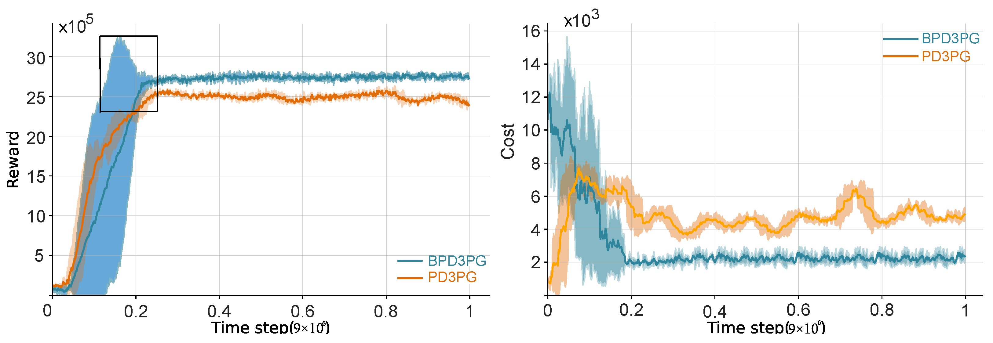
• Extensive simulations are conducted to investigate the dynamic responses of FCC under different operating conditions. Compared with traditional deterministic gradient methods, the proposed approach achieved improved economic profits and more stable control performance.

The remainder of this paper is structured as follows: Section 2 introduces the Constrained Markov Decision Process (CMDP); Section 3 elaborates on the proposed Bayesian SRL method; Section 4 presents the operation problem of FCC and the implementation details of the SRL scheme; Section 5 describes the results, and Section 6 concludes this paper.

2. Constrained Markov Decision Process

In this paper, we perform operational optimization of chemical processes using the SRL. The decision-maker, which is referred to as the agent in SRL, interacts with the environment by outputting actions according to some rules (the policy), such that the received cumulative rewards are maximized while satisfying process constraints (minimizing cumulative costs). SRL is typically tackled within the theoretical framework of the Constrained Markov Decision Process (CMDP) [17], defined by the state space $\mathcal{S}$, action space $\mathcal{A}$, state transition probability $\mathcal{P}\left(s_{t+1}\right|s_t,a_t)$ denoting the probability of transiting from state $s_t$ to $s_{t+1}$ given action $a_t$, reward function $r:\mathcal{S}\times \mathcal{A}\to \mathcal{R}$, cost function $c:\mathcal{S}\times \mathcal{A}\to \mathcal{R}$ representing the price for the constraint, the safety threshold d, and the discount factor $\gamma \in (0,1]$.

Suppose that the agent starts at the initial state following distribution, $s_0\sim l$, at each time step t, and it observes the current state $s_t$ and selects an action $a_t=\pi (·|s_t)$ according to the policy $\pi$. The agent receives an immediate reward $r_t=r(s_t,a_t)$ and immediate cost $c_t=c(s_t,a_t)$. After executing the action, the environment transitions to a new state $s_{t+1}$ according to the transition probability $\mathcal{P}\left(s_{t+1}\right|s_t,a_t)$. The above interaction procedure continues and generates a trajectory sequence $\mathcal{T}=\{s_0,a_0,r_0,c_0,s_1,a_1,r_1,c_1,\dots \}$. The agent’s cumulative discounted reward and cost are represented as $Z_{\pi }^R={\mathbb{E}}_{\mathcal{T}\sim \pi }{\sum }_{t=0}^{\infty }{\gamma }^t{r}_t$ and $Z_{\pi }^C={\mathbb{E}}_{\mathcal{T}\sim \pi }{\sum }_{t=0}^{\infty }{\gamma }^t{c}_t$, respectively.

The agent aims to learn an optimal safe policy ${\pi }^{*}$ that maximizes the expected cumulative reward $Z_{\pi }^R$ while satisfying the constraint $Z_{\pi }^C\le d$. This optimization problem can be formally expressed as

$${\pi }^{*}=\arg \underset{\pi }{\max }{Z}_{\pi }^R\mathrm{s}.\mathrm{t}.Z_{\pi }^C\le d$$

(1)

The CMDP problem (1) can typically be solved using the primal-dual method [18] by transforming it into the following dual form:

$${\pi }^{*}=\arg \underset{\pi }{\max }\underset{\mathcal{I}\ge 0}{\min }=Z_{\pi }^R-\mathcal{I}(Z_{\pi }^C-d)$$

(2)

where $\mathcal{I}\ge 0$ is the Lagrangian multiplier. The primal-dual method performs gradient ascent on $\pi$ and descent on $\mathcal{I}$ alternatively.

3. Bayesian Primal-Dual Deep Deterministic Policy Gradient

The core of actor–critic RL method lies in evaluating policy effectiveness through value functions. Value functions quantify the long-term rewards from specific actions in certain states, primarily including the state value function $V\left(s\right)$ or the state–action value function $Q(s,a)$, which are considered effective for problems with continuous state and action spaces, such as chemical process control. However, applying these methods to FCC units presents several challenges. First, in uncertain environments, value functions (critic) may provide inaccurate feedback, causing the actor to update in the wrong direction, leading to potentially low-reward samples [19]. While there might be a probability of achieving higher rewards, this often comes at the cost of constraint violations, which is absolutely unacceptable in actual chemical production. Furthermore, chemical reactions typically have irreversible characteristics, meaning that early incorrect decisions may lead to irreparable consequences. Therefore, building a value network that can accurately evaluate the environment becomes particularly important.

Given the advantages of Bayesian deep learning in handling uncertainties, we propose a natural extension: using BNNs as function approximators to model the complex nonlinear relationships between states and values [20].

3.1. Bayesian Neural Network

The neural networks define the mapping function $f_{\omega }:x\mapsto y$ from input space to output space, where $\omega$ are the parameterized weights. In the traditional neural networks, $\omega$ are deterministic parameters. The BNN employs probabilistic weights to quantify prediction uncertainty. As shown in Figure 1, $\omega$ in BNNs are random variables rather than fixed values. In the SRL, input x corresponds to state–action pairs $(s,a)$, and output y corresponds to Q-values Z; thus, our mapping function can be represented as $f_{\omega }:(s,a)\mapsto Z$. Given the dataset $\mathcal{D}$ (the evidence), we first specify a prior distribution for the weights (typically Gaussian), then perform Bayesian inference based on the likelihood function $p(Z\mid s,a,\omega )$ to obtain the posterior distribution of the weights:

$$p\left(\omega \right|\mathcal{D})={\displaystyle \frac{p\left(Z\right|s,a;\omega \left)p\right(\omega )}{\int p\left(Z\right|s,a;\omega \left)p\right(\omega )d\omega }}$$

(3)

Computing the posterior distribution $p\left(\omega \right|\mathcal{D})$ of BNN is a challenging problem. Various approximate inference methods have been proposed, including MCMC sampling [21], variational inference [22], expectation propagation [23], and Monte Carlo dropout approximation [24]. Notably, dropout has demonstrated excellent performance as a variational Bayesian method across multiple tasks, from classification to active learning, and will be deployed in this paper.

Based on the obtained the posterior distribution, the expected Q-value, namely $\mathbb{E}\left[Z\right(s,a\left)\right]$, for a new state–action pair $(s,a)$ can be estimated through MC sampling.

$$\begin{array}{cc}\hfill \mathbb{E}\left[Z\right(s,a\left)\right]& =\int f_{\omega }(s,a)p\left(\omega \right|\mathcal{D})d\omega \approx {\displaystyle \frac{1}{M}}\sum _{m=1}^M{f}_{{\omega }_m}(s,a)\hfill \end{array}$$

(4)

where M is the number of samples, ${\omega }_m\sim p\left(\omega \right|\mathcal{D})$.

3.2. Variational Inference in BNN with $\alpha$-Divergences

To simplify the computation of posterior distribution $p\left(\omega \right|\mathcal{D})$, variational inference introduces the variational distribution $q_{\theta }\left(\omega \right)$ as an approximation for $p\left(\omega \right|\mathcal{D})$. $q_{\theta }\left(\omega \right)$ is parameterized by $\theta$, typically taking the form of a Gaussian distribution: $q_{\theta }\left(\omega \right)=\mathcal{N}\left(\omega \right|\mu ,\sigma )$ (where $\theta =\{\mu ,\sigma \}$). A well-known approximation method is to minimize the Kullback–Leibler (KL) divergence between these two distributions as follows:

$$\begin{array}{cc}\hfill \arg \underset{\theta }{\min }\mathrm{KL}[q_{\theta }\left(\omega \right)\left|\right|p\left(\omega \right|\mathcal{D})]& =\arg \underset{\theta }{\min }\int q_{\theta }\left(\omega \right)\log {\displaystyle \frac{q_{\theta }\left(\omega \right)}{p\left(\omega \right|\mathcal{D})}}\mathrm{d}\omega \hfill \end{array}$$

(5)

$$\begin{array}{cc}\hfill & =\arg \underset{\theta }{\min }\int q_{\theta }\left(\omega \right)\log {\displaystyle \frac{q_{\theta }\left(\omega \right)}{p\left(\omega \right)p(\mathcal{D}\mid \omega )/p\left(\mathcal{D}\right)}}\mathrm{d}\omega \hfill \end{array}$$

(6)

$$\begin{array}{cc}\hfill & =\arg \underset{\theta }{\min }\mathrm{KL}\underset{-ELBO\left(q\right)}{\underbrace{[q_{\theta }\left(\omega \right)\parallel p\left(\omega \right)]-\mathbb{E}{q}_{\theta }\left(\omega \right)\left[\log p(\mathcal{D}\mid \omega )\right]}}+\underset{Const}{\underbrace{\log p\left(\mathcal{D}\right)}}.\hfill \end{array}$$

(7)

where the first term on the right-hand side of the last equality is known as the evidence lower bound (ELBO).

Although the optimization method described above is theoretically simple and intuitive, it still faces significant computational complexity challenges in practical implementation. Dropout can serve as an alternative approach for Bayesian approximation [25]. Dropout can be interpreted as a unique form of variational inference that introduces noise into the feature space, which maps to uncertainty in the network parameter space. Specifically, during training, dropout randomly “drops” some neurons by applying stochastic masks to network weights, thereby approximating the probability distribution of parameters. At test time, dropout is applied to all neurons to approximate Bayesian inference. This method can effectively capture model uncertainty while maintaining computational efficiency.

On the other hand, dropout variational inference tends to underestimate model uncertainty. This issue stems from the asymmetric penalty mechanism in KL divergence minimization: penalties are applied when the approximate posterior distribution $q_{\theta }\left(\omega \right)$ assigns non-zero values in regions where the true posterior distribution $p\left(\omega \right|\mathcal{D})$ is zero. However, no penalties are imposed when $q_{\theta }\left(\omega \right)$ is zero in regions where $p\left(\omega \right|\mathcal{D})$ has high probability.

To address this limitation, inspired by [26], we adopt the $\alpha$-divergence as an alternative measure:

$$D_{\alpha }\left[p\right|\left|q\right]={\displaystyle \frac{1}{\alpha (1-\alpha )}}\left(1-\int p{\left(\omega \right|\mathcal{D})}^{\alpha }{q}_{\theta }{\left(\omega \right)}^{1-\alpha }d\omega \right)$$

(8)

As illustrated in Figure 2, the parameter $\alpha$ influences the characteristics of approximate distributions. In principle, the method is a generalization with the tunable parameter $\alpha$. When $\alpha$ takes a large positive value, the approximate distribution $q_{\theta }\left(\omega \right)$ tends to encompass multiple modes of the target distribution $p\left(\omega \right|\mathcal{D})$. Conversely, as $\alpha$ approaches negative infinity (assuming finite divergence), $q_{\theta }\left(\omega \right)$ focuses on the dominant mode with the highest probability [27].

Several effective $\alpha$-divergence minimization techniques, such as Black-Box $\alpha$-Divergence Minimization (BB-$\alpha$) [27] and dropout BB-$\alpha$ [26], have reportedly achieved significant results in practical applications. Notably, BB-$\alpha$, as a black-box method, can be directly applied to probability models with complex structures. This characteristic is particularly important in cases where traditional methods such as variational Bayes, expectation propagation (EP), and Power EP encounter difficulties when processing energy functions. First, let us review the traditional BB-$\alpha$ function.

$${\mathcal{L}}_{\alpha }^{MC}\left(q_{\theta }\left(\omega \right)\right)=-{\displaystyle \frac{1}{\alpha }}\sum _t\log \left[{\left({\displaystyle \frac{p\left(y\right|x;\omega )p_0{\left(\omega \right)}^{\frac{1}{T}}}{q_{\theta }{\left(\omega \right)}^{\frac{1}{T}}}}\right)}^{\alpha }\right]$$

(9)

however, due to the intractability of its general expectation form, to improve computational efficiency and better adapt to gradient-based optimization, we approximate the expectation value by drawing samples from the distribution $q_{\theta }\left(\omega \right)$ and reformulate this objective function (9) using MC method:

$$\begin{array}{cc}\hfill {\mathcal{L}}_{\alpha }^{MC}& =-{\displaystyle \frac{1}{\alpha }}\log E_{\omega \sim q_{\theta }\left(\omega \right)}\left[{\left({\displaystyle \frac{p\left(y\right|x;\omega )p_0\left(\omega \right)}{q_{\theta }\left(\omega \right)}}\right)}^{\alpha }\right]\hfill \end{array}$$

(10)

$$\begin{array}{cc}\hfill & \approx -{\displaystyle \frac{1}{\alpha }}\sum _t\log E_{\omega \sim q_{\theta }\left(\omega \right)}\left[\exp \left(\alpha \log p\left(y_t\right|x_t;\omega )+{\displaystyle \frac{\alpha }{T}}[\log p_0\left(\omega \right)-\log q_{\theta }\left(\omega \right)]\right)\right]\hfill \end{array}$$

(11)

$$\begin{array}{cc}\hfill & \approx -{\displaystyle \frac{1}{\alpha }}\sum _t\log \sum _m^M\exp \left(\alpha \log p\left(y_t\right|x_t;{\omega }_m)+{\displaystyle \frac{\alpha }{T}}[\log p_0\left({\omega }_m\right)-\log q_{\theta }\left({\omega }_m\right)]\right)\hfill \end{array}$$

(12)

Given a loss function $l(.)$, we define the un-normalized likelihood term: $p\left(y\right|x,\omega )\propto \exp \left[-l(y,f_{\omega }\left(x\right))\right]$ [28]. The term $\log p_0\left({\omega }_m\right)$ represents the log prior, equivalent to $l_1$ or $l_2$ regularization [29]. We provide the following minimization objective:

$${\mathcal{L}}_{\alpha }^{MC}\approx -{\displaystyle \frac{1}{\alpha }}\sum _t\log \sum _m^M\exp \left(-\alpha l(y,f_{{\omega }_m}\left(x\right))+{\displaystyle \frac{\alpha }{T}}[l_2-\log q_{\theta }\left({\omega }_m\right)]\right)$$

(13)

The log-likelihood term $-l(y,f_{\omega }\left(x\right))$ can be cross-entropy for classification tasks. However, in our value regression task, it is represented as mean squared error: $-l(y,f_{\omega }\left(x\right))\propto -{\displaystyle \frac{\beta }{2}}\left|\right|y-f_{\omega }(s,a){\left|\right|}_2^2$, where the corresponding likelihood term can be expressed as $y\sim \mathcal{N}(y;f_{\omega }(s,a),{\beta }^{-1}\sigma )$ [26]. By reformulating the energy function (13), we derive a new objective function representation method called $\alpha$-BNN, which can approximate the marginal likelihood with high precision and is compatible with mainstream objective functions in deep learning.

The new optimization objective of $\alpha$-BNN is

$$\begin{array}{cc}\hfill {\mathcal{L}}_{\alpha }^{MC}\left(q_{\theta }\left(\omega \right)\right)& =-{\displaystyle \frac{1}{\alpha }}\sum _t\log \sum _{m=1}^M\exp \left[-{\displaystyle \frac{\alpha \beta }{2}}{\parallel y_t-f_{{\omega }_m}(s,a)\parallel }_2^2\right]+{\displaystyle \frac{ND}{2}}\log \beta +\sum _i{p}_i{\parallel H_i\parallel }_2^2\hfill \end{array}$$

(14)

where $\beta$ represents the precision parameter, weight samples ${\widehat{\omega }}_m\sim q_{\theta }\left(\omega \right)$ are obtained through masked dropout, and ${\left\{f_{{\omega }_m}(s,a)\right\}}_{m=1}^M$ represents a set of forward propagations obtained by performing K sampling iterations on input $(s,a)$. D and $p_i$. denote the dropout rate and retention rate of the i-th layer, respectively, N is the batch size, and H represents the network parameters without dropout.

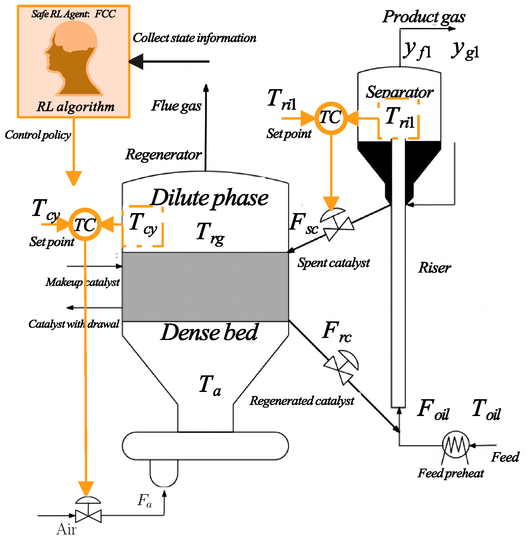
4. The Fluid Catalytic Cracking Process

4.1. Process Descriptions

The FCC process consists of three stages: reaction, product separation, and catalyst regeneration (Figure 3). Crude oil mixes with a hot recycled catalyst from the regenerator on the feed side and enters the riser. The catalyst’s heat vaporizes the oil and enables cracking. In the riser, heavy oil cracks into lighter hydrocarbons, mainly gasoline, which are separated from the catalyst and sent to the fractionator. The multicomponent catalyst typically contains acid USHY zeolite, active alumina matrix, inert matrix (kaolin), binder, and additives. During the reaction, coke deposits deactivate the catalyst, so it is returned to the regenerator to burn off the coke and restore activity. In the regenerator, air is blown from the bottom to fluidize the catalyst, mixing it well with air in the dense bed. Makeup catalyst and withdrawal flows compensate for permanent catalyst losses. The regenerated catalyst is recycled to mix with fresh crude oil feed. A cyclone at the regenerator top separates and collects solid catalyst from the flue gas [30].

The core mechanism of catalytic cracking is the $\beta$-scission reaction, which fundamentally generates olefins and new carbocations by cleaving $\beta$ carbon–carbon bonds. During this process, carbocations undergo chain reactions with alkane molecules, continuously producing short-chain olefins. Typical reaction pathways include $C_{16}{H}_{34}\to C_8{H}_{18}+C_8{H}_{16},C_8{H}_{18}\to C_4{H}_{10}+C_4{H}_8$, among many others. Given the extreme complexity of the cracking reaction network, its intrinsic mechanism remains incompletely elucidated, making the construction of a comprehensive first-principle model extremely challenging. Currently, FCC models predominantly employ hybrid approaches combining reaction mechanisms with empirical rules, with lumped models being the most practical and widely used. This research adopts the three-lumped reactor model [30]. The model abstracts FCC reactions as transitions between three virtual lumped components: gas oil (F) cracking to generate gasoline (G) and light gases/coke (L), with conversion pathways including $F\to G,G\to L,F\to L$.

The riser model is approximated as steady-state ordinary differential equations (quasi-steady state), while the regenerator is described by differential equations derived from material and energy balance relationships. For detailed derivation and explanation of these equations, readers are referred to Guan et al. [30].

Table 1. Model parameters of the FCC unit.

Variable	Description	Value and Unit
$E_{cb}$	Activation energy for coke burning reaction	158.6 kJ/mol
$F_{oil}$	Mass flow rate of gas oil feed	2438.0 kg/min
$F_{gl}$	Gasoline yield factor of catalyst	1.0 kg/min
$k_c$	Rate constant for catalytic coke formation	0.01897 ${\mathrm{s}}^{-0.5}$
$k_{com}$	Rate constant for coke burning	29.338 ${\min }^{-1}$
$k_o$	Rate constant for gas oil cracking	962,000 ${\mathrm{s}}^{-1}$
$T_a$	Temperature of air to regenerator	320.0 K
$T_{oil}$	Temperature of gas oil feed	420.0 K
${\sigma }_2$	CO2/CO dependence on the temperature	0.006244 ${\mathrm{K}}^{-1}$
$h_1$, $h_2$	Parameters for approximating $\Delta H$	521,150.0, 245.0

lists the material prices for FCC components used in economic profit calculations, while

Table 2. Process variables of the FCC unit.

Variable	Description	Unit
$F_a$	Mass flow rate of air to regenerator	kg/min
$F_{sc}$	Mass flow rate of spent catalyst	kg/min
$T_{rg}$	Temperature of catalyst in regenerator dense bed	K
$T_{cy}$	Temperature of cyclone	K
$T_{ri0}$	Temperature of catalyst and gas oil mixture at riser inlet	K
$T_{ri1}$	Temperature of catalyst and gas oil mixture at riser outlet	K
$y_{f1}$	Weight fraction of gas oil in product	-
$y_{gl}$	Weight fraction of gasoline in product	-

and

Table 3. Material prices for FCC components.

Price	Component	Value
$p_{gl}$	gasoline	0.14 USD/kg
$p_{gs}$	light gases	0.132 USD/kg
$p_{ugo}$	unconverted gas oil	0.088 USD/kg

list the key process variables and model parameters.

To facilitate the subsequent transformation of the FCC problem into the required reinforcement learning framework, the following key constraints and economic objective function need to be clearly defined.

The input capacity constraints are

$$6000\mathrm{kg}/\min \le F_{sc}\le 24,000\mathrm{kg}/\min$$

(15)

$$0\le F_a\le 3600\mathrm{kg}/\min$$

(16)

Metallurgical limit for the temperature of cyclone:

$$T_{cy}\le 1000\mathrm{K}$$

(17)

Metallurgical limits for the riser inlet and outlet:

$$T_{ri0}\le 1000\mathrm{K}$$

(18)

$$T_{ri1}\le 1000\mathrm{K}$$

(19)

The economic profit function, J [USD/min], is defined as

$$J=p_{gl}{F}_{gl}+p_{gs}{F}_{gs}+p_{ugo}{F}_{ugo}-p_{ugo}{F}_{oil}$$

(20)

and the overall operational objective can be formulated as solving the following problem:

$$\begin{array}{cc}\hfill & \underset{F_{sc},F_a}{\max }J=p_{gl}{F}_{gl}+p_{gs}{F}_{gs}+p_{ugo}{F}_{ugo}-p_{ugo}{F}_{oil}\hfill \\ \hfill & s.t.\mathrm{constraints}:\left(15\right)–\left(19\right)\hfill \end{array}$$

(21)

We consider the process parameters ${[k_o,k_c,k_{com},{\sigma }_2,h_1,h_2,Ecb/R]}^T$ as uncertain (see Table 1 for nominal values). Under nominal conditions, nonlinear programming optimization yields optimal $F_{sc}=17,189\mathrm{kg}/\min$ and $F_a=1461.7\mathrm{kg}/\min$, with a maximum profit of 44.96 USD/min. However, this solution only applies to nominal conditions. During actual operation, uncertain disturbances cause continuous changes in operating conditions, potentially making pre-determined schemes suboptimal or infeasible [30].

4.2. Formulating as a SRL Problem

The FCC process under consideration is described as a two-degree-of-freedom system ($F_{sc}$ and $F_a$) [31,32], whose objective is to maximize the economic profit while satisfying constraints (15)–(19). Given the complex dynamic characteristics, multiple operational constraints, and clear economic objectives of the FCC process, it is handled by applying SRL in this study. As previously described, we formalize the FCC control problem as a CMDP, with its core components detailed below.

(1) $Agent$: The agent serves as the intelligence achieving optimal control under complex operating conditions through continuous interactive learning. During each sampling period t, the system acquires key state parameters from the sensors (observations). The interaction between the agent and the FCC process generates a control sequence $\mathcal{T}$, with a total of T periods.

Let $X\in R,C,x\in r,c$, and the state–action value function ${\mathcal{G}}_{\pi ,\mathcal{I}}(s,a,\omega )$ characterizes the expected economic profit that can be obtained when executing policy $\pi$ and control action $a_t$ in state $s_t$ while satisfying operational constraints. We solve the optimal value function

$${\pi }^{*}=\underset{{\mathcal{G}}_{\pi ,\mathcal{I}}(s,a,\omega )}{\underbrace{Z_{\pi }^R(s,a;\omega )-\mathcal{I}{Z}_{\pi }^C(s,a;\omega )}}$$

(22)

Based on this, the FCC unit implements policy ${\pi }^{*}$ for optimal control. To achieve maximum cumulative profit throughout the entire process, the agent must continuously learn and refine the mapping relationship between system states and optimal control actions through ongoing interaction with the controlled object.

(2) $State$: The state vector $s_t$ is the feedback signal to the SRL agent, reflecting the set of process parameters of the FCC environment after executing control command $a_{t-1}$ at sampling period $t-1$; the state space is defined as follows:

$$s_t=[t,C_{rc},O_d,T_{rg},T_{ri1},y_{f1},y_{g1},T_{ri0},J,T_{cy}]\in \mathcal{S}$$

(23)

where t denotes the time step within the training period. The detailed parameters of the state space $\mathcal{S}$ are listed in Table 1 and Table 2.

(3) $Action$: Given state $s_t$, the corresponding control action $a_t$ taken by the SRL agent at time step t is defined as

$$a_t=[a_t^{F_{sc}},a_t^{F_a}]\in \mathcal{A}$$

(24)

where $a_t^{F_{sc}}\in$ [6000, 24,000] represents the catalyst circulation rate, and $a_t^{F_a} \in [0,3600]$ represents the regenerator air flow rate.

(4) $EnvironmentandStateTransition$: Once the action $a_t$ is outputted, the agent interacts with the fluid catalytic cracking environment to obtain the next state $s_{t+1}$ and receives reward $r_t$ and cost $c_t$. This interaction process can be represented by the mapping function $[s_{t+1},r_t,c_t]=f_{FCC}(s_t,a_t)$, which is constrained by operational rules and governed by relevant physical laws to ensure the feasibility of the action selected at each time step.

(5) $RewardandCost$: In Formula (20), the terms represent product profit and raw material costs, respectively. p represents the material price, as shown in Table 3. Therefore, the overall operational objective can be formulated as solving the following optimization problem to maximize cumulative rewards:

$$r_t=p_{gl}{F}_{gl}+p_{gs}{F}_{gs}+p_{ugo}{F}_{ugo}-p_{ugo}{F}_{oil}$$

(25)

Based on the characteristics and constraints of the FCC process (15)–(19), the cost signals are designed as

$$\left\{\begin{array}{cc}{c}_{T_{cy,t}}={\lambda }_1(T_{cy,t}-1000),\hfill & \mathrm{if}{T}_{cy,t}>1000\hfill \\ c_{T_{ri0,t}}={\lambda }_2(T_{ri0,t}-1000),\hfill & \mathrm{if}{T}_{ri0,t}>1000\hfill \\ c_{T_{ri1,t}}={\lambda }_3(T_{ri1,t}-1000),\hfill & \mathrm{if}{T}_{ri1,t}>1000\hfill \\ c_{{F_{sc,t}}_1}={\lambda }_4(F_{sc,t}-24,000),\hfill & \mathrm{if}{F}_{sc,t}>24,000\hfill \\ c_{{F_{sc,t}}_2}={\lambda }_5(6000-F_{sc,t}),\hfill & \mathrm{if}{F}_{sc,t}<6000\hfill \\ c_{F_{a,t}}={\lambda }_6(F_{a,t}-3600),\hfill & \mathrm{if}{F}_{a,t}>3600\hfill \\ 0,\hfill & \mathrm{otherwise}\hfill \end{array}\right.$$

(26)

$$\begin{array}{cc}\hfill c_{t1}& ={\lambda }_7\left(T_{ri1}-782.8\right)+{\lambda }_8\left(T_{cy}-999.5\right)\hfill \end{array}$$

(27)

$$\begin{array}{cc}\hfill c_t& =c_{T_{cy,t}}+c_{T_{ri0,t}}+c_{T_{ri1,t}}+c_{{F_{sc,t}}_1}\hfill \\ \hfill & +c_{{F_{sc,t}}_2}+c_{F_{a,t}}+c_{t1}\hfill \end{array}$$

(28)

where $\lambda$ is a tunable bias constant.

5. Simulation Results

5.1. Training Algorithms

We carry out comparative experiments between the primal-dual version of the standard DDPG [33] (PD3PG) and the Bayesian PD3PG (BPD3PG). Considering the specificity of the application scenario, which involves a multi-dimensional continuous action space, traditional Deep Q-Network (DQN) [34] and Deep Policy Gradient (DPG) [35] algorithms cannot address such challenges. As mentioned previously, we employ the primal-dual method to solve the CMDP problem. Although traditional reinforcement learning algorithms such as DDPG can also attempt to solve this problem, the constraints present in practical applications make the direct application of these algorithms infeasible.

Our network is based on the actor–critic architecture of DDPG, with two modifications made through the primal-dual method. First, we add a cost critic to the existing reward critic to estimate the expected cumulative cost. Second, for the actor, we incorporate the optimization of the cost Q-value and maximize the reward Q-value. Regarding the implementation details, we constructed six deep neural networks (DNNs) for the online and target actors, reward critics, and cost critics. To ensure the comparability and reproducibility of the experiments, PD3PG and BPD3PG adopt identical structural configurations (more details of the parameters are shown in

Table 4. Hyper-parameters of the proposed BPD3PG and PD3PG.

Parameter	Value
Hidden layer	64-128-64
Batch size	64
Time step	9 × 106
Episode	2000
MC sample (Only for BPD3PG)	50
Dropout rate (Only for BPD3PG)	0.995
Actor-learning rate	0.0001
Reward/Cost-learning rate	0.0001
Discount factor	0.99
$\alpha$-divergence (Only for BPD3PG)	0.95
KeepProp (Only for BPD3PG)	0.95
$\beta$ (Only for BPD3PG)	0.92

and

Table 5. Hardware details.

Parameter	Version
Computer	Windows10
CPU	i5-12400F 2.50 GHz
RAM	32.0 GB
GPU	NVIDIA GeForce RTX4060Ti
Tensorflow	2.2.0
Python	3.8

and Algorithm 1). We employ $\alpha$-Bayesian neural networks ($\alpha$-BNNs) as the Q-value functions. Following the aforementioned loss calculation strategy, our goal is to capture the uncertainty estimates of the Q-value functions accurately. The fitting target for the $\alpha$-BNN Q-function is

$$y_t=g+\gamma ·Z^{\prime X}(s_{t+1},{\pi }_{{\varphi }^{\prime }}\left(s_{t+1}\right))$$

where ${\varphi }^{\prime }$ represents the target policy, and $Z^{\prime }$ corresponds to the target network adjusted through a soft update mechanism. We update the BPD3PG using the MC dropout posterior mean of the Bayesian value function distribution, replacing the deterministic estimate.

$$\begin{array}{c}\hfill {\nabla }_{\varphi }{J}_{{\pi }_{\varphi }}\approx {\displaystyle \frac{1}{M}}\sum _{m=1}^M\left[{\nabla }_{\varphi }{\pi }_{\varphi }\left(s\right){\nabla }_a{\mathcal{G}}_{{\pi }_{\varphi },\mathcal{I}}(s,a;{\omega }_m)\right]{|}_{s=s_t}\end{array}$$

(29)

where ${\mathcal{G}}_{{\pi }_{\varphi },\mathcal{I}}(s,a,\omega )=Z_{\pi }^R(s,a;\omega )-\mathcal{I}{Z}_{\pi }^C(s,a;\omega )$; similarly, the value of the Lagrangian multiplier $\mathcal{I}$ can be determined by minimizing the loss function ${\nabla }_{\varphi }{J}_{\mathcal{I}}$.

$$\begin{array}{c}\hfill {\nabla }_{\varphi }{J}_{\mathcal{I}}\approx {\displaystyle \frac{1}{M}}\sum _{m=1}^M\left[{\nabla }_{\varphi }{\pi }_{\varphi }\left(s\right){\nabla }_a\mathcal{I}(Z_{\pi }^C(s,a;{\omega }_m)-d)\right]{|}_{s=s_t}\end{array}$$

(30)

The training processes of BDP3PG and PD3PG are compared in Figure 4, where one observes that BDP3PG outperforms PD3PG with higher reward and lower cost. Furthermore, as seen in Figure 4, by fitting the $\alpha$-BNN value function and using the posterior mean in the policy update, BPD3PG demonstrates faster convergence and improved stability, particularly in disturbed settings. This improvement can be attributed to the stronger exploration ability demonstrated by BPD3PG when faced with high uncertainty during the early stages of learning.

Algorithm 1 BPD3PG

Input: Initial netowrk $Z_{\pi }^R,Z_{\pi }^C,{\pi }_{\varphi }$ Input: Target parameters: $\{Z_{\pi }^R,Z_{\pi }^C,{\pi }_{{\varphi }^{\prime }}\}\leftarrow \{Z_{\pi }^R,Z_{\pi }^C,{\pi }_{\varphi }\}$ Input: Initial replay buffer $\mathcal{X}$ and Lagrangian multiplier $\mathcal{I}$   1:   for each episode do   2:         for each time step do   3:               $a={\pi }_{\varphi }\left(s_t\right)$   4:               $s_{t+1}\sim \mathcal{P}(·|s_t,a_t)$   5:               $\mathcal{X}\leftarrow \mathcal{X}\cup (s_t,a_t,r_t,c_t,s_{t+1})$   6:         end for   7:         for each gradient step do   8:               Sample experience from replay buffer $\mathcal{X}$   9:               Update the reward and cost critic network by minimizing the loss function (14). 10:              Update the Lagrangian multiplier using (30). 11:              Update the actor network using (29). 12:              Update the target network soft update [33] 13:        end for 14:  end for Output: $Z_{\pi }^R,Z_{\pi }^C,{\pi }_{\varphi },\mathcal{I}$

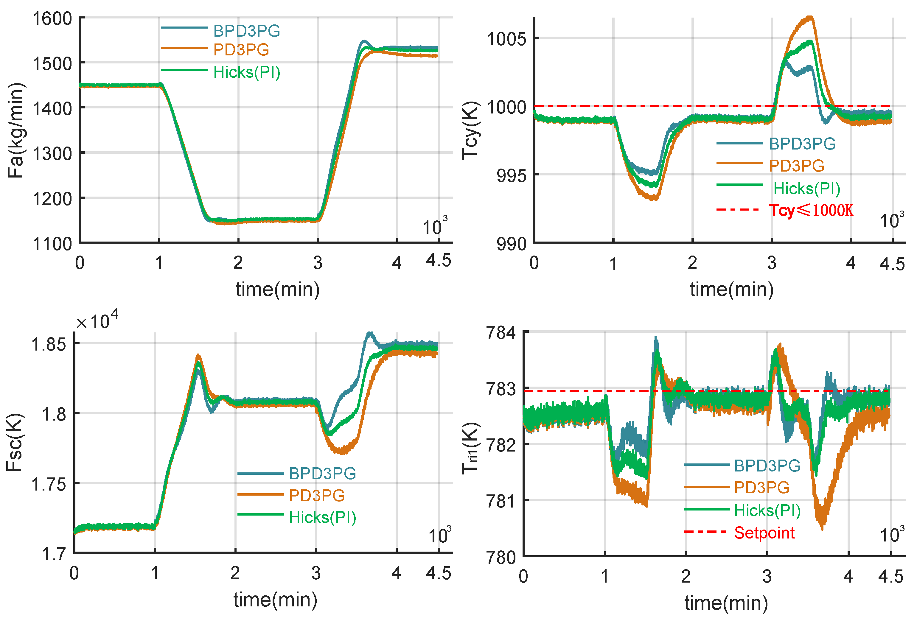
5.2. Experimental Results

As shown in Figure 3, the traditional control structure is based on the Hicks framework, which has pairing relationships of $F_{sc}\leftrightarrow T_{ri1}$ and $F_a\leftrightarrow T_{cy}$. According to the research by [13], this pairing relationship provides optimal controllability. In this study, the RL is additionally configured to optimize the control signals, as shown in Figure 3. As an active constraint variable, $T_{cy}$ requires special attention in both deep reinforcement learning control schemes.

The simulation experiments are arranged as follows: Initially, the FCC process operates under nominal conditions. To simulate the parameter fluctuations typically encountered in industrial processes, two disturbance scenarios, ${\mathbf{d}}_{\mathbf{1}}$ and ${\mathbf{d}}_{\mathbf{2}}$, are introduced, representing random variations in key model parameters within $\pm 20\%$ of their nominal values.

Specifically, the parameter vector ${[k_o,k_c,k_{com},{\sigma }_2,h_1,h_2,Ecb/R]}^T$ (refer to Table 1) under nominal conditions is

$${\mathbf{d}}_{\mathbf{0}}={[962000,0.01897,29.338,0.006244,521150,245,158.6]}^T$$

At $t=1000$ min, a disturbance scenario

$${\mathbf{d}}_{\mathbf{1}}={[743903.8231,0.01666,31.5,0.0070,497882,274.8,162.6]}^T$$

is introduced smoothly via a 500 min ramp function. At $t=3000$ min, the scenario switches to another value

$${\mathbf{d}}_{\mathbf{2}}={[995340.7075,0.01663,28.8,0.00665,537683,196.8,163.5]}^T$$

We compared the performance of two SRL-based control methods, BPD3PG and PD3PG, under both undisturbed and disturbed conditions:

• Undisturbed condition: The system operates in an ideal control environment. The manipulated variables $F_{sc}$ and $F_a$ are precisely regulated by the controller, while the key parameters change according to disturbance scenarios ${\mathbf{d}}_{\mathbf{1}}$ and ${\mathbf{d}}_{\mathbf{2}}$, but no random disturbances or measurement noises are introduced.
• Disturbed condition: In addition to the key parameter changes following disturbance scenarios ${\mathbf{d}}_{\mathbf{1}}$ and ${\mathbf{d}}_{\mathbf{2}}$, the system is also subject to random disturbances. Specifically, the manipulated variables become $F_{sc}+{\delta }_{sc}$ and $F_a+{\delta }_a$, and the measured variables become $T_{cy}+{\eta }_{cy}$ and $T_{ri1}+{\eta }_{ri1}$, where $\delta \sim \mathcal{N}(0,20)$ and the noise power $\eta =[0.1^2]\times 1$.

The dynamic tracking performances are shown in Figure 5 and Figure 6, respectively. Overall, both controllers track their respective control variables reasonably well under the influence of disturbances. Moreover, the practical constraint $T_{cy}$ remains close to 999.5 K for most of the time, efficiently meeting the requirement $T_{cy}\le 1000$ K. An exception occurs around 3000 min when the introduction of disturbance ${\mathbf{d}}_{\mathbf{2}}$ causes $T_{cy}$ to significantly exceed the limit. However, compared to PD3PG, BPD3PG exhibits greater robustness. Through continuous interaction with the environment, trial and error, and feedback learning, BPD3PG returns $T_{cy}$ within the feasible range after 3000 min. In another control loop, the reactor temperature $T_{ri1}$ is stabilized near the set-point of 782.8 K by manipulating $F_{sc}$.

In terms of economic performance, Figure 7 shows the profit function J under both disturbed and undisturbed conditions for the two methods using the Hicks control structure. The BPD3PG method usually achieves higher economic profits, especially when disturbances are present, highlighting its superior robustness. Under nominal conditions (0–1000), the economic profits of both methods are nearly identical (nominal optimum). This is expected because no particular adaptations are needed for both cases. However, in the ${\mathbf{d}}_{\mathbf{1}}$ scenario (1000–3000), the profit of BPD3PG ($J_{undisturbed}^{BPD3PG}=42.11$/$J_{disturbed}^{BPD3PG}=42.05$) is significantly higher than that of PD3PG ($J_{undisturbed}^{PD3PG}=41.87$/$J_{disturbed}^{PD3PG}=41.74$). For the ${\mathbf{d}}_{\mathbf{2}}$ scenario, the final settlement results for both methods show that the economic profit of BPD3PG ($J_{undisturbed}^{BPD3PG}=49.31$/$J_{disturbed}^{BPD3PG}=49.33$) consistently outperforms PD3PG ($J_{undisturbed}^{PD3PG}=48.94$/$J_{disturbed}^{PD3PG}=48.44$). Moreover, comparing with the Hicks control structure implemented with PI controllers, our BPD3PG method achieved notably higher profits ($J_{disturbed}^{Hicks}=48.96/J_{disturbed}^{BPD3PG}=49.33$), demonstrating the economic advantages of our approach.

In contrast, PD3PG shows a larger profit difference between disturbed and undisturbed conditions, indicating weaker robustness. In contrast, the profit difference for BPD3PG is smaller between noisy and undisturbed conditions, with some fluctuation, but, overall, it consistently outperforms both PD3PG and traditional control approaches (shown in

Table 6. Performance improvement of BPD3PG in the final settlement results.

Comparison	Condition	J (USD/min)	Improvement (%)
BPD3PG vs. Hicks	Undisturbed	49.31 vs. 49.11	0.41%↑
	Disturbed	49.33 vs. 48.96	0.76%↑
BPD3PG vs. PD3PG	Undisturbed	49.31 vs. 48.94	0.76%↑
	Disturbed	49.33 vs. 48.44	1.84%↑

).

6. Conclusions

This paper presented a Bayesian deep reinforcement learning method for the optimization of chemical processes, called the Bayesian Primal-Dual Deep Deterministic Policy Gradient (BPD3PG) method, which is successfully applied to a fluid catalytic cracking (FCC) unit. The BPD3PG employs Bayesian neural networks for value function approximation, which effectively captured the uncertainties in FCC processes and overcame the value function overestimation problem inherent in traditional deterministic deep reinforcement learning. Furthermore, by utilizing the primal-dual method to handle process constraints, this approach ensured the operational feasibility of the system.

The simulation experiments on the FCC unit validated the superior performance of the BPD3PG method. The BPD3PG significantly outperformed traditional PI controllers, as well as deterministic policy gradient methods, achieving higher economic profits (Table 6) and maintaining more stable process control performance, especially when facing significant disturbance scenarios that could potentially cause controller overreaction.

References

1. Bloor, M.; Ahmed, A.; Kotecha, N.; Mercangöz, M.; Tsay, C.; Chanona, E.A.D.R. Control-Informed Reinforcement Learning for Chemical Processes. Ind. Eng. Chem. Res. 2025, 64, 4966–4978. [Google Scholar] [CrossRef] [PubMed]
2. Karniadakis, G.E.; Kevrekidis, I.G.; Lu, L.; Perdikaris, P.; Wang, S.; Yang, L. Physics-informed Machine Learning. Nat. Rev. Phys. 2021, 3, 422–440. [Google Scholar] [CrossRef]
3. Byun, H.E.; Kim, B.; Lee, J.H. Embedding Active Learning in Batch-to-batch Optimization Using Reinforcement Learning. Automatica 2023, 157, 111260. [Google Scholar] [CrossRef]
4. Oh, T.H.; Park, H.M.; Kim, J.W.; Lee, J.M. Integration of reinforcement learning and model predictive control to optimize semi-batch bioreactor. AIChE J. 2022, 68, e17658. [Google Scholar] [CrossRef]
5. Syauqi, A.; Kim, H.; Lim, H. Optimizing Olefin Purification: An Artificial Intelligence-Based Process-Conscious PI Controller Tuning for Double Dividing Wall Column Distillation. Chem. Eng. J. 2024, 500, 156645. [Google Scholar] [CrossRef]
6. Petukhov, A.N.; Shablykin, D.N.; Trubyanov, M.M.; Atlaskin, A.A.; Zarubin, D.M.; Vorotyntsev, A.V.; Stepanova, E.A.; Smorodin, K.A.; Kazarina, O.V.; Petukhova, A.N.; et al. A hybrid batch distillation/membrane process for high purification part 2: Removing of heavy impurities from xenon extracted from natural gas. Sep. Purif. Technol. 2022, 294, 121230. [Google Scholar] [CrossRef]
7. Singh, V.; Kodamana, H. Reinforcement Learning Based Control of Batch Polymerisation Processes. IFAC-PapersOnLine 2020, 53, 667–672. [Google Scholar] [CrossRef]
8. Hartlieb, M. Photo-iniferter RAFT polymerization. Macromol. Rapid Commun. 2022, 43, 2100514. [Google Scholar] [CrossRef]
9. Chen, J.; Wang, F. Cost Reduction of CO2 Capture Processes Using Reinforcement Learning Based Iterative Design: A Pilot-Scale Absorption–stripping System. Sep. Purif. Technol. 2013, 122, 149–158. [Google Scholar] [CrossRef]
10. Perera, A.T.D.; Wickramasinghe, P.U.; Nik, V.M.; Scartezzini, J.L. Introducing Reinforcement Learning to the Energy System Design Process. Appl. Energy 2020, 262, 114580. [Google Scholar] [CrossRef]
11. Sachio, S.; Mowbray, M.; Papathanasiou, M.M.; del Rio-Chanona, E.A.; Petsagkourakis, P. Integrating Process Design and Control Using Reinforcement Learning. Chem. Eng. Res. Des. 2021, 183, 160–169. [Google Scholar] [CrossRef]
12. Kim, S.; Jang, M.G.; Kim, J.K. Process Design and Optimization of Single Mixed-Refrigerant Processes with the Application of Deep Reinforcement Learning. Appl. Therm. Eng. 2023, 223, 120038. [Google Scholar] [CrossRef]
13. Hicks, R.; Worrell, G.; Durney, R. Atlantic seeks improved control; studies analog-digital models. Oil Gas J. 1966, 24, 97. [Google Scholar]
14. Boum, A.T.; Latifi, A.; Corriou, J.P. Model predictive control of a fluid catalytic cracking unit. In Proceedings of the 2013 International Conference on Process Control (PC), Strbske Pleso, Slovakia, 18–21 June 2013; IEEE: Piscataway, NJ, USA, 2013; pp. 335–340. [Google Scholar]
15. Skogestad, S. Plantwide control: The search for the self-optimizing control structure. J. Process Control 2000, 10, 487–507. [Google Scholar] [CrossRef]
16. Ye, L.; Cao, Y.; Yuan, X. Global approximation of self-optimizing controlled variables with average loss minimization. Ind. Eng. Chem. Res. 2015, 54, 12040–12053. [Google Scholar] [CrossRef]
17. Altman, E. Constrained Markov Decision Processes; Chapman and Hall/CRC: Boca Raton, FL, USA, 1999. [Google Scholar]
18. Ji, J.; Zhou, J.; Zhang, B.; Dai, J.; Pan, X.; Sun, R.; Huang, W.; Geng, Y.; Liu, M.; Yang, Y. OmniSafe: An Infrastructure for Accelerating Safe Reinforcement Learning Research. J. Mach. Learn. Res. 2024, 25, 1–6. [Google Scholar]
19. Yoo, H.; Kim, B.; Kim, J.W.; Lee, J.H. Reinforcement Learning Based Optimal Control of Batch Processes Using Monte-Carlo Deep Deterministic Policy Gradient with Phase Segmentation. Comput. Chem. Eng. 2021, 144, 107133. [Google Scholar] [CrossRef]
20. Kaelbling, L.P.; Littman, M.L.; Moore, A.W. Reinforcement learning: A survey. J. Artif. Intell. Res. 1996, 4, 237–285. [Google Scholar] [CrossRef]
21. Neal, R.M. Bayesian Learning for Neural Networks; Springer Science & Business Media: Berlin/Heidelberg, Germany, 2012; Volume 118. [Google Scholar]
22. Graves, A. Practical variational inference for neural networks. Adv. Neural Inf. Process. Syst. 2011, 24, 2348–2356. [Google Scholar]
23. Minka, T.P. Expectation propagation for approximate Bayesian inference. arXiv 2013, arXiv:1301.2294. [Google Scholar]
24. Gal, Y.; McAllister, R.; Rasmussen, C.E. Improving PILCO with Bayesian neural network dynamics models. In Proceedings of the Data-Efficient Machine Learning Workshop, ICML, New York, NY, USA, 24 June 2016; Volume 4, p. 25. [Google Scholar]
25. Henderson, P.; Doan, T.; Islam, R.; Meger, D. Bayesian Policy Gradients via Alpha Divergence Dropout Inference. In Proceedings of the NIPS Bayesian Deep Learning Workshop, Long Beach, CA, USA, 4–9 December 2017. [Google Scholar]
26. Li, Y.; Gal, Y. Dropout Inference in Bayesian Neural Networks with Alpha-divergences. In Proceedings of the 34th International Conference on Machine Learning, Sydney, Australia, 6–11 August 2017; pp. 2052–2061. [Google Scholar]
27. Hernandez-Lobato, J.; Li, Y.; Rowland, M.; Bui, T.; Hernández-Lobato, D.; Turner, R. Black-box alpha divergence minimization. In Proceedings of the International Conference on Machine Learning, PMLR, New York, NY, USA, 19–24 June 2016; pp. 1511–1520. [Google Scholar]
28. LeCun, Y.; Chopra, S.; Hadsell, R.; Ranzato, M.; Huang, F. A tutorial on energy-based learning. In Predicting Structured Data; MIT Press: Cambridge, MA, USA, 2006; Volume 1. [Google Scholar]
29. Liu, X.; Sun, S. Alpha-divergence Minimization with Mixed Variational Posterior for Bayesian Neural Networks and Its Robustness Against Adversarial Examples. Neurocomputing 2020, 423, 427–434. [Google Scholar] [CrossRef]
30. Guan, H.; Ye, L.; Shen, F.; Song, Z. Economic Operation of a Fluid Catalytic Cracking Process Using Self-Optimizing Control and Reconfiguration. J. Taiwan Inst. Chem. Eng. 2019, 96, 104–113. [Google Scholar] [CrossRef]
31. Loeblein, C.; Perkins, J. Structural design for on-line process optimization: II. Application to a simulated FCC. AIChE J. 1999, 45, 1030–1040. [Google Scholar] [CrossRef]
32. Hovd, M.; Skogestad, S. Procedure for regulatory control structure selection with application to the FCC process. AIChE J. 1993, 39, 1938–1953. [Google Scholar] [CrossRef]
33. Lillicrap, T.P.; Hunt, J.J.; Pritzel, A.; Heess, N.; Erez, T.; Tassa, Y.; Silver, D.; Wierstra, D. Continuous control with deep reinforcement learning. arXiv 2015, arXiv:1509.02971. [Google Scholar]
34. Mnih, V.; Kavukcuoglu, K.; Silver, D.; Rusu, A.A.; Veness, J.; Bellemare, M.G.; Graves, A.; Riedmiller, M.; Fidjeland, A.K.; Ostrovski, G.; et al. Human-level control through deep reinforcement learning. Nature 2015, 518, 529–533. [Google Scholar] [CrossRef]
35. Silver, D.; Lever, G.; Heess, N.; Degris, T.; Wierstra, D.; Riedmiller, M. Deterministic policy gradient algorithms. In Proceedings of the International Conference on Machine Learning, PMLR, Beijing, China, 22–24 June 2014; pp. 387–395. [Google Scholar]
Figure 1. (1) Traditional neural network; (2) Bayesian neural network.
Processes 13 01352 g001
Figure 2. An illustration of approximating distributions by α -divergence minimization. Here, p and q shown in the graphs are un-normalized probability densities.
Processes 13 01352 g002
Figure 3. The fluid catalytic cracking unit with RL agent.
Processes 13 01352 g003
Figure 4. The shaded region represents half a standard deviation of the average evaluation over 5 trials. Curves are smoothed uniformly for visual clarity.
Processes 13 01352 g004
Figure 5. Optimal trajectories after RL training and dynamic simulation of the Hicks control structure: loop1( F a T c y ) and loop2( F s c T r i 1 ) (undisturbed).
Processes 13 01352 g005
Figure 6. Optimal trajectories after RL training and dynamic simulation of the Hicks control structure: loop1( F a T c y ) and loop2( F s c T r i 1 ) (disturbed).
Processes 13 01352 g006
Figure 7. Dynamic trajectories of the economic function J (disturbed and undisturbed).
Processes 13 01352 g007