
Total Model-Free Robust Control of Non-Affine Nonlinear Systems with Discontinuous Inputs


Abstract
1. Introduction
- (1)
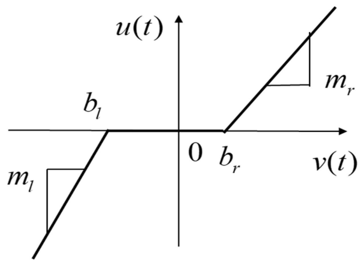
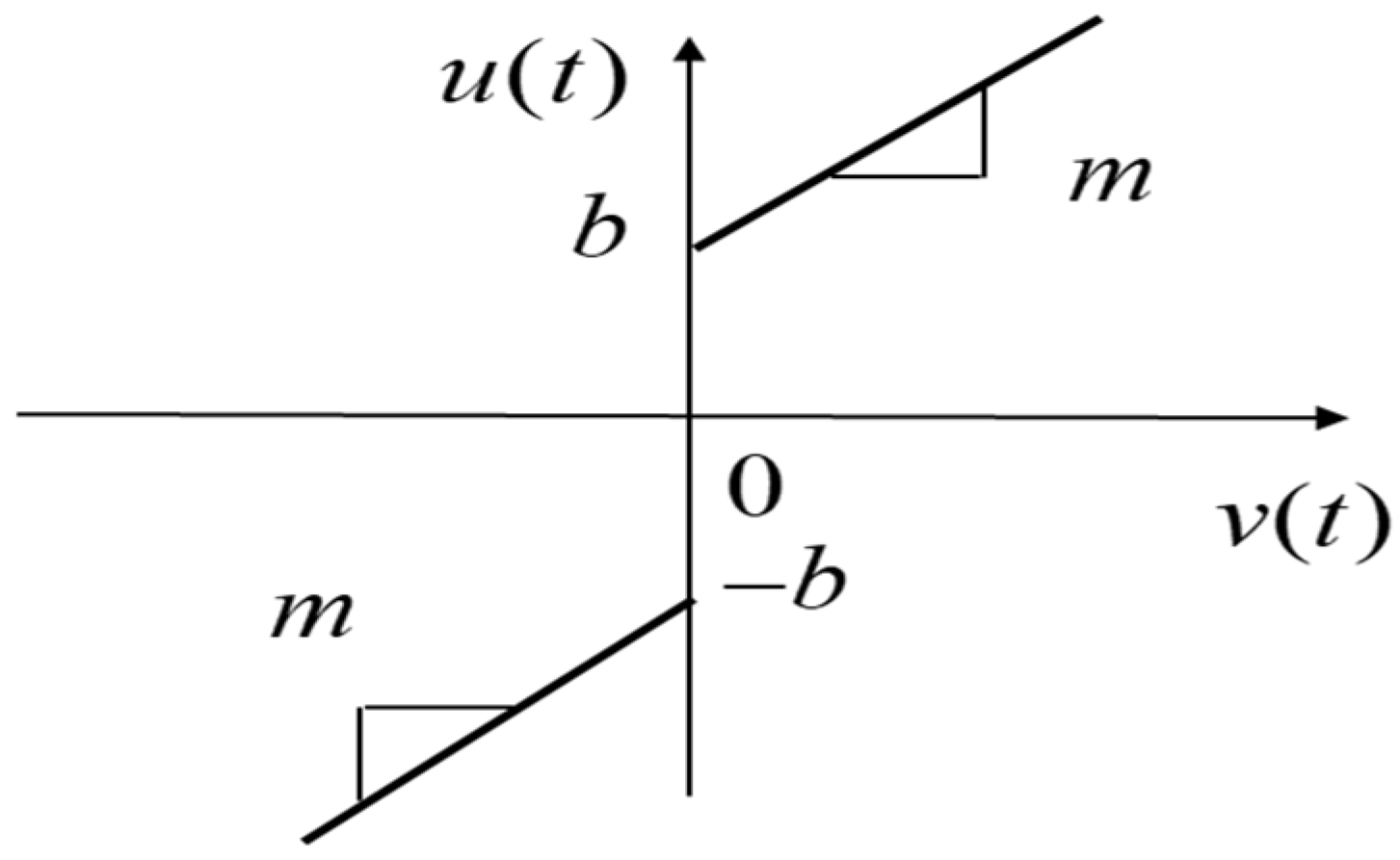
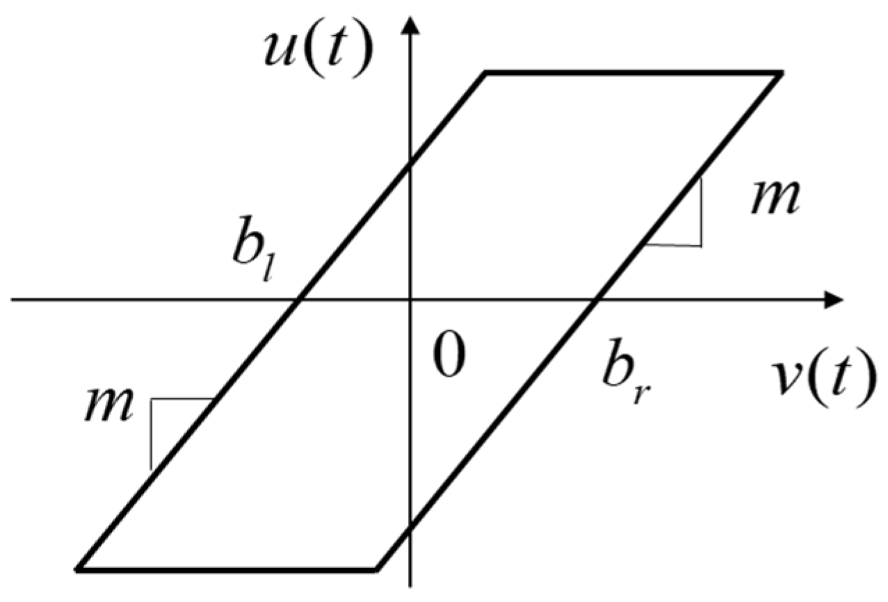
- Establishing a total model-free robust control by taking plant and discontinuous inputs as a whole uncertainty for the control. Therefore, the approach is applicable to many discontinuous inputs, e.g., dead zone, friction, or backlash, without knowing the nonlinear input function.
- (2)
- Extending the MFSMC to piecewise continuous system control. A control Lyapunov function (CLF) for non-affine control systems is created [32] using a sliding mode manifold (SMM) for an unknown model plant. Moreover, a sensitivity function is defined to address its robustness, which is a complement to the model-based sensitivity function.
- (3)
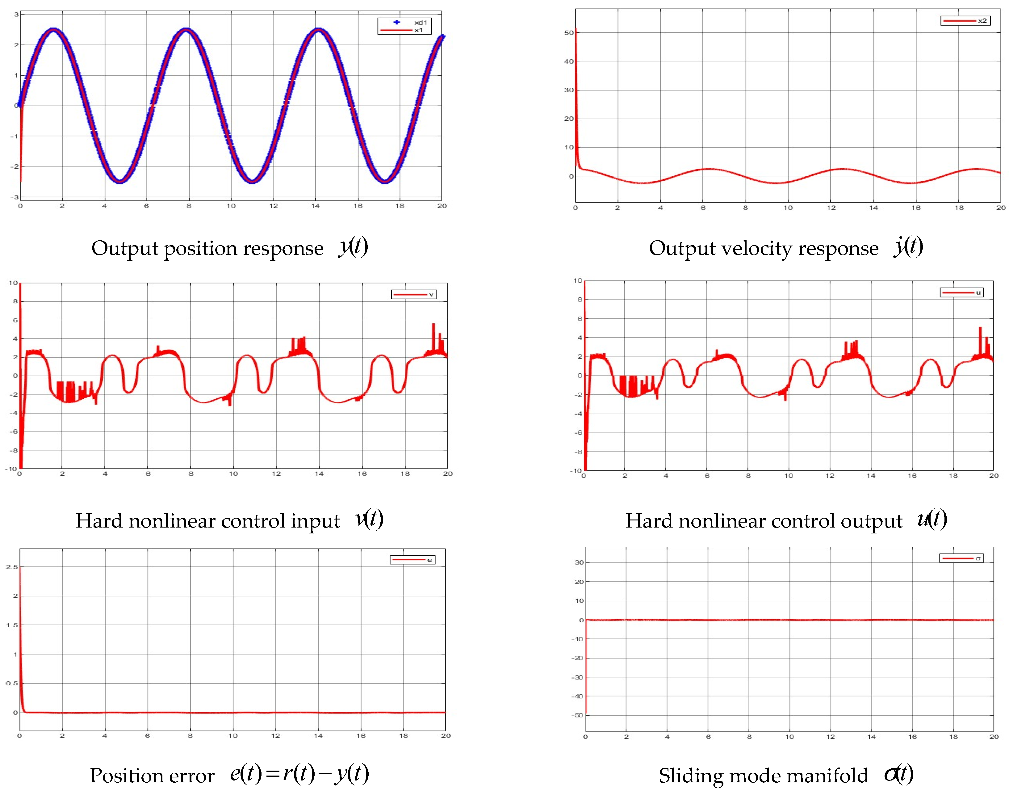
- Providing comprehensive simulation demonstrations and real lab tests to verify the feasibility and efficiency of the TMFRC in controlling unknown nonlinear plants with hard nonlinear inputs.
2. Problem Statement and Preliminaries
2.1. Dynamic System with Input Discontinuities
2.2. Control Problem Statement
3. TMFRC of Nonlinear Systems with Discontinuous Input
3.1. Sliding Mode Control (SMC) with Continuous Inputs
3.2. Model-Free Sliding Mode Control (MFSMC) with Discontinuous Inputs
- (1)
- Assign a linear sliding mode manifold as
- (2)
- The model-free equivalent controller is designed by
3.3. Existence of TMFRC
3.4. Implementation of Controller
3.4.1. Proportional (P) Function
3.4.2. Proportional and Integral (PI) Function
3.4.3. Monotone Bounded Logistic Function
3.5. Sensitivity Analysis
4. Simulation and Experimental Demonstrations
4.1. Simulations
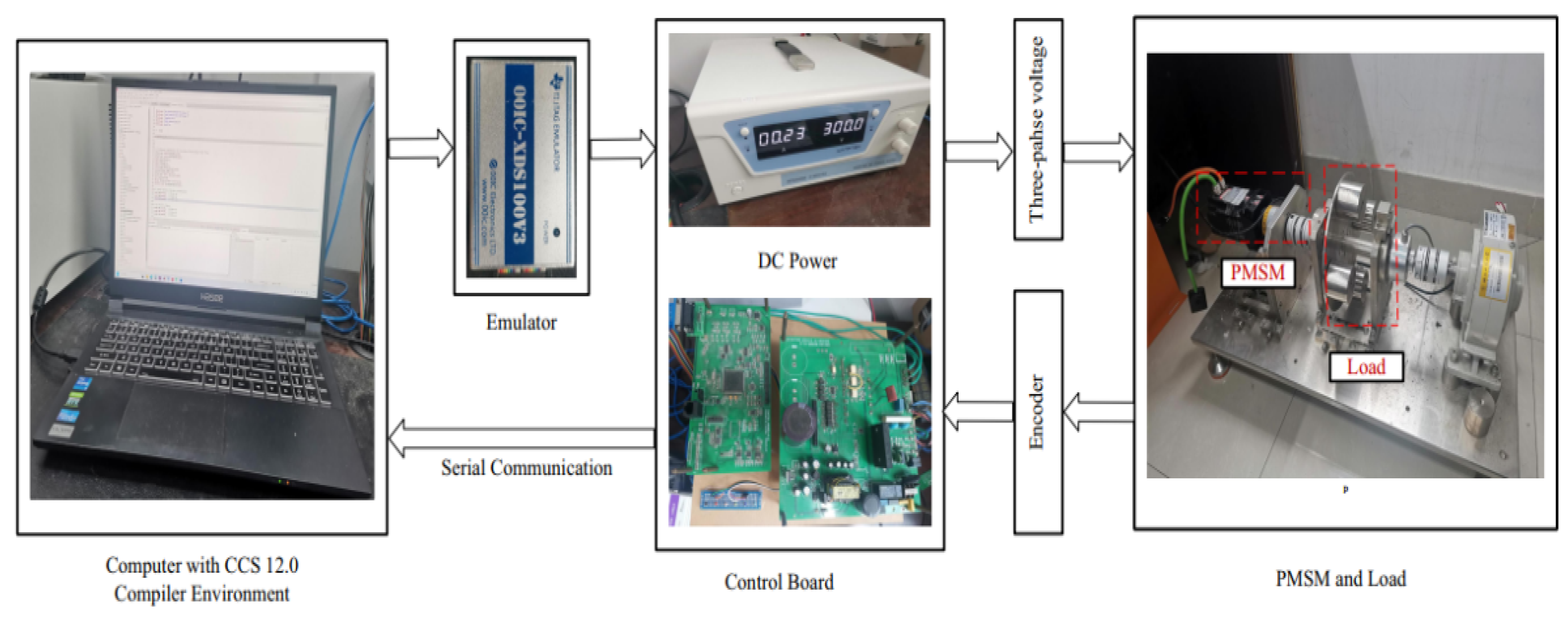
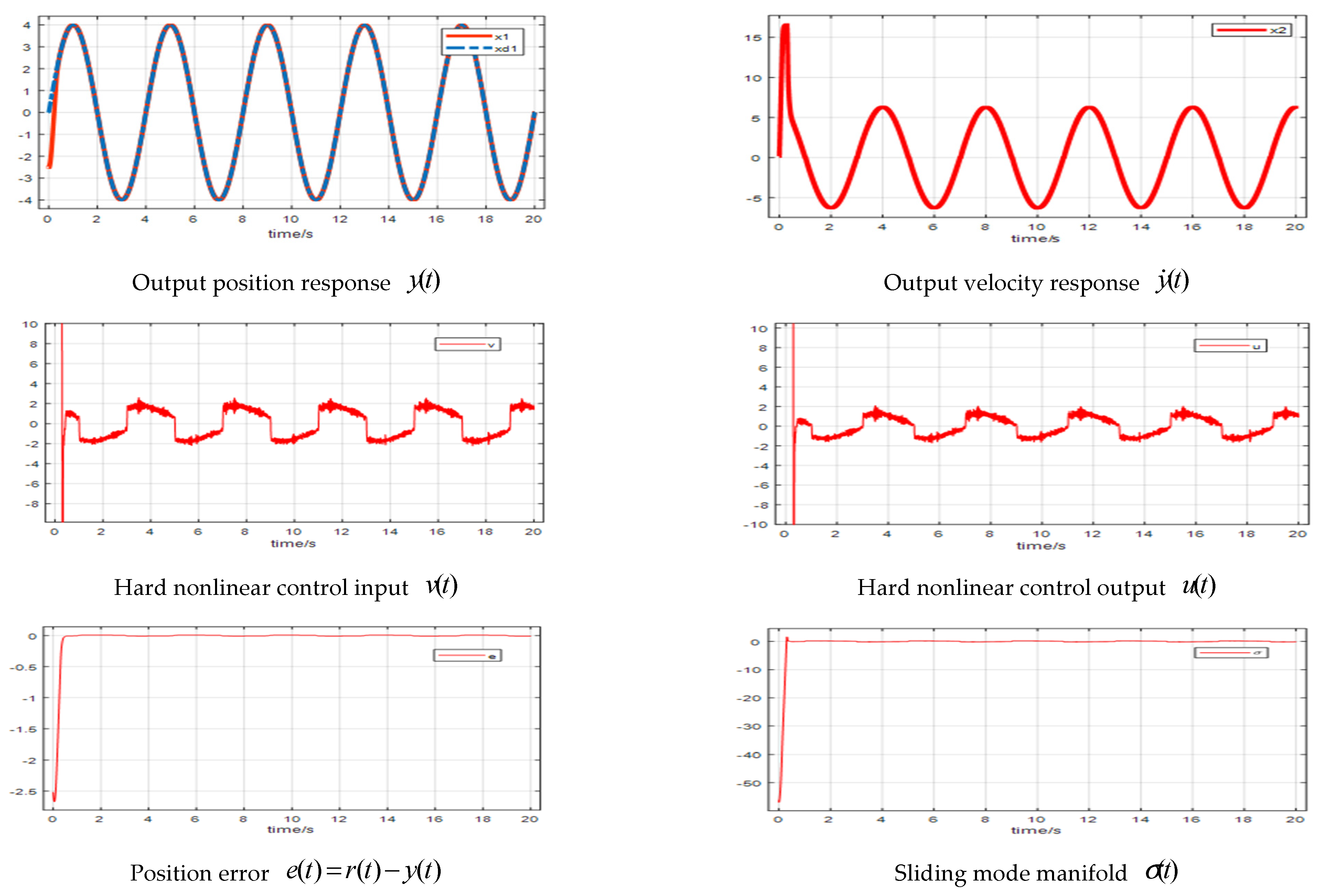
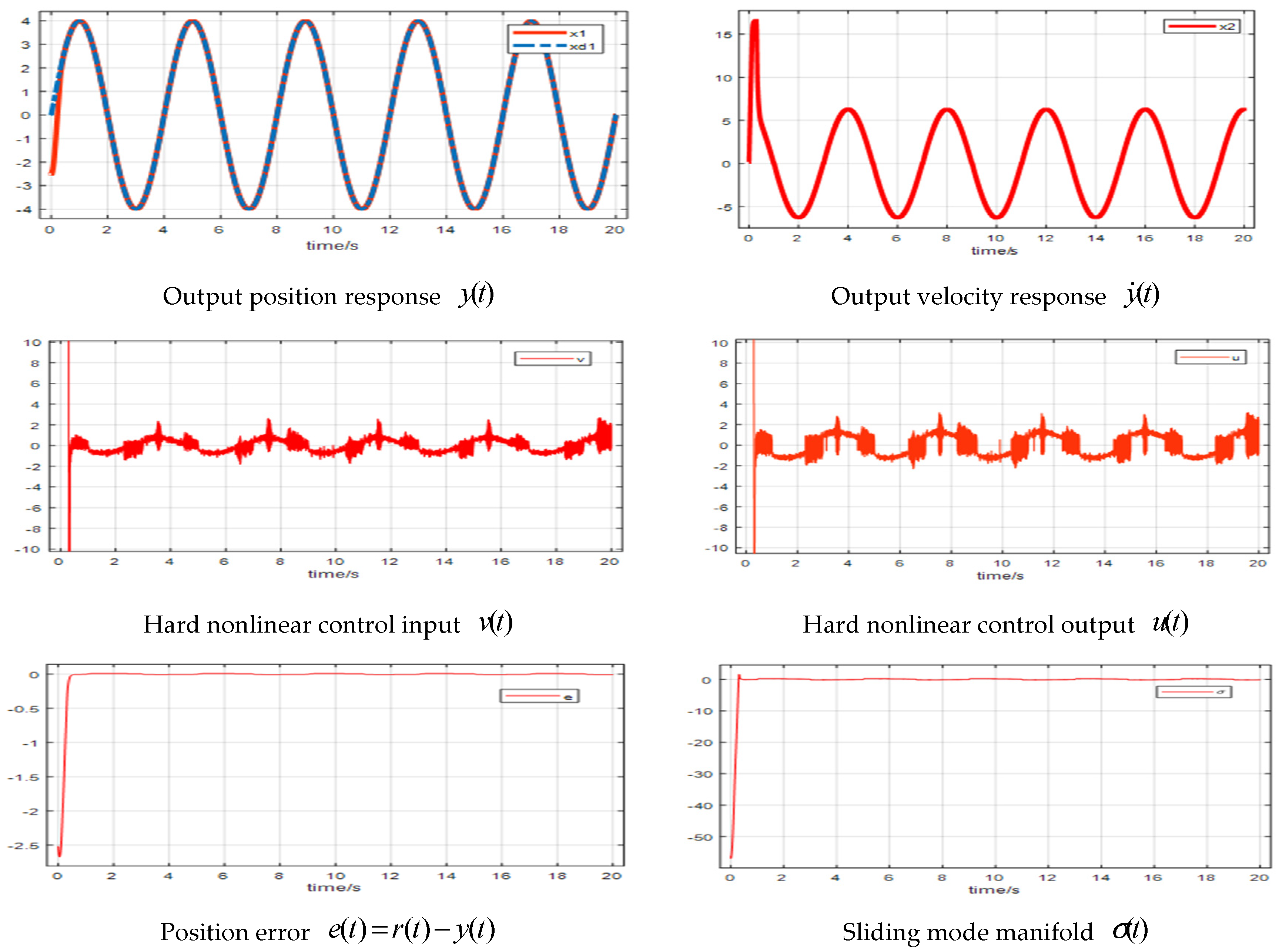
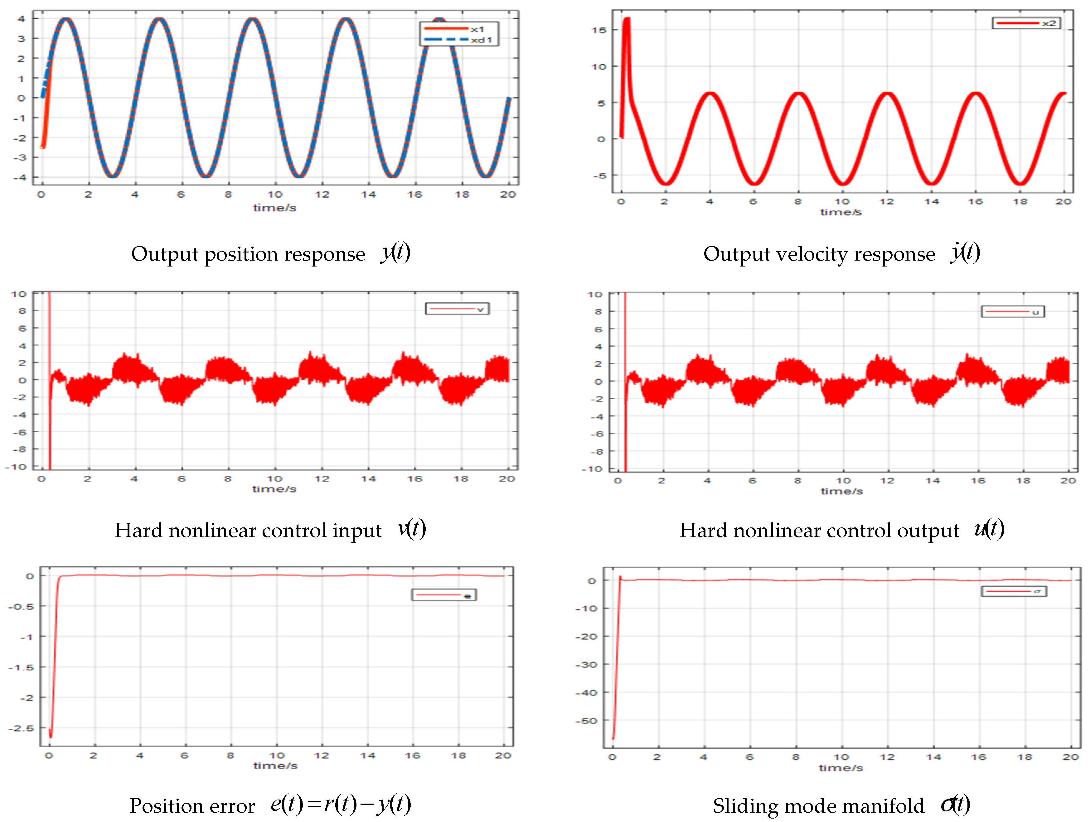
4.2. Experiments
5. Conclusions
Author Contributions
Funding
Data Availability Statement
Acknowledgments
Conflicts of Interest
References
- Na, J.; Chen, Q.; Ren, X. Adaptive Identification and Control of Uncertain Systems with Non-Smooth Dynamics; Academic Press: Cambridge, MA, USA, 2018; pp. xvii–xviii. [Google Scholar]
- Orlov, Y.V. Discontinuous Systems; Springer: London, UK, 2009. [Google Scholar]
- Kunze, M.; Küpper, T. Non-Smooth Dynamical Systems: An Overview. In Ergodic Theory, Analysis, and Efficient Simulation of Dynamical Systems; Springer: Berlin/Heidelberg, Germany, 2001; pp. 431–452. [Google Scholar]
- Sabarianand, D.V.; Karthikeyan, P.; Muthuramalingam, T. A review on control strategies for compensation of hysteresis and creep on piezoelectric actuators based micro systems. Mech. Syst. Signal Process. 2020, 140, 106634. [Google Scholar] [CrossRef]
- Gang, T.; Kokotovic, P.V. Adaptive control of plants with unknown dead-zones. IEEE Trans. Autom. Control 1994, 39, 59–68. [Google Scholar] [CrossRef]
- Tao, G.; Kokotović, P.V. Discrete-time adaptive control of plants with unknown output dead-zones. Automatica 1995, 31, 287–291. [Google Scholar] [CrossRef]
- Zhou, J.; Wen, C.; Zhang, Y. Adaptive output control of nonlinear systems with uncertain dead-zone nonlinearity. IEEE Trans. Autom. Control 2006, 51, 504–511. [Google Scholar] [CrossRef]
- Lai, G.; Tao, G.; Zhang, Y.; Liu, Z. Adaptive Control of Noncanonical Neural-Network Nonlinear Systems with Unknown Input Dead-Zone Characteristics. IEEE Trans. Neural Netw. Learn. Syst. 2020, 31, 3346–3360. [Google Scholar] [CrossRef]
- Wu, L.-B.; Yang, G.-H.; Wang, H.; Wang, F. Adaptive fuzzy asymptotic tracking control of uncertain nonaffine nonlinear systems with non-symmetric dead-zone nonlinearities. Inf. Sci. 2016, 348, 1–14. [Google Scholar] [CrossRef]
- Wang, X.-S.; Su, C.-Y.; Hong, H. Robust adaptive control of a class of nonlinear systems with unknown dead-zone. Automatica 2004, 40, 407–413. [Google Scholar] [CrossRef]
- Ma, H.-J.; Yang, G.-H. Adaptive output control of uncertain nonlinear systems with non-symmetric dead-zone input. Automatica 2010, 46, 413–420. [Google Scholar] [CrossRef]
- Hu, T.; Lin, Z. Control Systems with Actuator Saturation: Analysis and Design; Springer: Berlin/Heidelberg, Germany, 2001. [Google Scholar]
- Åström, K.J. Control of systems with friction. In Proceedings of the Fourth International Conference on Motion and Vibration Control, Zurich, Switzerland, 25–28 August 1998; pp. 25–32. [Google Scholar]
- Fang, S.; Hu, C.; Hu, X.; Zhang, Z. Switched sliding mode approach for motion control systems with friction. Proc. Inst. Mech. Eng. Part I J. Syst. Control Eng. 2017, 231, 513–526. [Google Scholar] [CrossRef]
- Khan, Z.A.; Chacko, V.; Nazir, H. A review of friction models in interacting joints for durability design. Friction 2017, 5, 1–22. [Google Scholar] [CrossRef]
- Zhou, J.; Zhang, C.; Wen, C. Robust Adaptive Output Control of Uncertain Nonlinear Plants with Unknown Backlash Nonlinearity. IEEE Trans. Autom. Control 2007, 52, 503–509. [Google Scholar] [CrossRef]
- Hassani, V.; Tjahjowidodo, T.; Do, T.N. A survey on hysteresis modeling, identification and control. Mech. Syst. Signal Process. 2014, 49, 209–233. [Google Scholar] [CrossRef]
- Lai, G.; Liu, Z.; Zhang, Y.; Chen, C.L.P.; Xie, S. Asymmetric Actuator Backlash Compensation in Quantized Adaptive Control of Uncertain Networked Nonlinear Systems. IEEE Trans. Neural Netw. Learn. Syst. 2017, 28, 294–307. [Google Scholar] [CrossRef]
- Phu, D.X.; Mien, V. Robust control for vibration control systems with dead-zone band and time delay under severe disturbance using adaptive fuzzy neural network. J. Frankl. Inst. 2020, 357, 12281–12307. [Google Scholar] [CrossRef]
- Tedone, F.; Palladino, M. Hamilton–Jacobi–Bellman Equation for Control Systems with Friction. IEEE Trans. Autom. Control 2021, 66, 5651–5664. [Google Scholar] [CrossRef]
- Zhao, Z.; Liu, Y.; Cai, S.; Li, Z.; Wang, Y.; Hong, K.-S. Adaptive Quantized Control of Flexible Manipulators Subject to Unknown Dead Zones. IEEE Trans. Syst. Man Cybern. Syst. 2023, 53, 6438–6447. [Google Scholar] [CrossRef]
- Tao, G. Multivariable adaptive control: A survey. Automatica 2014, 50, 2737–2764. [Google Scholar] [CrossRef]
- Chen, K.; Astolfi, A. Adaptive Control for Systems with Time-Varying Parameters—A Survey. In Trends in Nonlinear and Adaptive Control: A Tribute to Laurent Praly for His 65th Birthday; Jiang, Z.-P., Prieur, C., Astolfi, A., Eds.; Springer International Publishing: Cham, Switzerland, 2022; pp. 217–247. [Google Scholar]
- Huang, Y.; Xue, W. Active disturbance rejection control: Methodology and theoretical analysis. ISA Trans. 2014, 53, 963–976. [Google Scholar] [CrossRef]
- Feng, H.; Guo, B.-Z. Active disturbance rejection control: Old and new results. Annu. Rev. Control 2017, 44, 238–248. [Google Scholar] [CrossRef]
- Fareh, R.; Khadraoui, S.; Abdallah, M.Y.; Baziyad, M.; Bettayeb, M. Active disturbance rejection control for robotic systems: A review. Mechatronics 2021, 80, 102671. [Google Scholar] [CrossRef]
- Zhu, Q. Complete model-free sliding mode control (CMFSMC). Sci. Rep. 2021, 11, 22565. [Google Scholar] [CrossRef] [PubMed]
- Zhu, Q. Model-Free Sliding Mode Enhanced Proportional, Integral, and Derivative (SMPID) Control. Axioms 2023, 12, 721. [Google Scholar] [CrossRef]
- Zhu, Q.; Li, R.; Zhang, J. Model-free robust decoupling control of nonlinear nonaffine dynamic systems. Int. J. Syst. Sci. 2023, 54, 2590–2607. [Google Scholar] [CrossRef]
- Zhu, Q.; Mobayen, S.; Nemati, H.; Zhang, J.; Wei, W. A new configuration of composite nonlinear feedback control for nonlinear systems with input saturation. J. Vib. Control 2023, 29, 1417–1430. [Google Scholar] [CrossRef]
- Zhu, Q.; Zhang, W.; Li, S.; Chen, Q.; Na, J.; Ding, H. U-control—A universal platform for control system design with inversion/cancellation of nonlinearity, dynamic and coupling through model-based to model-free procedures. Int. J. Syst. Sci. 2025, 56, 484–501. [Google Scholar] [CrossRef]
- Bacciotti, A.; Ceragioli, F. Stability and Stabilization of Discontinuous Systems and Nonsmooth Lyapunov Functions. ESAIM COCV 1999, 4, 361–376. [Google Scholar] [CrossRef]
- Slotine, J.-J.E.; Li, W. Applied Nonlinear Control (No. 1); Prentice Hall: Englewood Cliffs, NJ, USA, 1991. [Google Scholar]
- Turner, M.C. Actuator deadzone compensation: Theoretical verification of an intuitive control strategy. Control Theory Appl. IEE Proc. 2006, 153, 59–68. [Google Scholar] [CrossRef]
- West, C.; Monk, S.D.; Montazeri, A.; Taylor, C.J. A Vision-Based Positioning System with Inverse Dead-Zone Control for Dual-Hydraulic Manipulators. In Proceedings of the 2018 UKACC 12th International Conference on Control (CONTROL), Sheffield, UK, 5–7 September 2018; pp. 379–384. [Google Scholar]
- Patton, R.J.; Putra, D.; Klinkhieo, S. Friction compensation as a fault-tolerant control problem. Int. J. Syst. Sci. 2010, 41, 987–1001. [Google Scholar] [CrossRef]
- Wang, J.; Ge, S.S.; Lee, T.H. Adaptive Friction Compensation for Servo Mechanisms. In Adaptive Control of Nonsmooth Dynamic Systems; Tao, G., Lewis, F.L., Eds.; Springer: London, UK, 2001; pp. 211–248. [Google Scholar]
- Acho, L.; Iurian, C.; Ikhouane, F.; Rodellar, J. Robust-Adaptive Control of Mechanical Systems with Friction: Application to an Industrial Emulator. In Proceedings of the 2007 American Control Conference, New York, NY, USA, 9–13 July 2007; pp. 5970–5974. [Google Scholar]
- Iyer, R.V.; Tan, X. Control of hysteretic systems through inverse compensation. IEEE Control Syst. Mag. 2009, 29, 83–99. [Google Scholar] [CrossRef]
- Guo, B.-Z.; Zhao, Z.-L. On the convergence of an extended state observer for nonlinear systems with uncertainty. Syst. Control Lett. 2011, 60, 420–430. [Google Scholar] [CrossRef]
- Molnár, T.; Cosner, R.; Singletary, A.; Ubellacker, W.; Ames, A. Model-Free Safety-Critical Control for Robotic Systems. IEEE Robot. Autom. Lett. 2022, 7, 944–951. [Google Scholar] [CrossRef]
- Wang, S.; Liu, Y.; Yu, H.; Chen, Q. Approximation-Free Control for Nonaffine Nonlinear Systems with Prescribed Performance. In Proceedings of the 2022 41st Chinese Control Conference (CCC), Hefei, China, 25–27 July 2022; pp. 2277–2282. [Google Scholar] [CrossRef]
- Eslami, M. Theory of Sensitivity in Dynamic Systems: An Introduction; Springer Science & Business Media: Berlin/Heidelberg, Germany, 2013. [Google Scholar]
- Iqbal, K. Introduction to Control Systems. 2021. Available online: https://eng.libretexts.org/Bookshelves/Industrial_and_Systems_Engineering/Introduction_to_Control_Systems_(Iqbal) (accessed on 6 April 2025).
- Jiang, C.; Sui, S.; Li, Y.; Tong, S. Adaptive NN Output Feedback Control of Electro-hydraulic System. Int. J. Control Autom. Syst. 2023, 21, 2739–2747. [Google Scholar] [CrossRef]


| Controller | Parameters |
|---|---|
| Names | Parameters | Values |
|---|---|---|
| Moment of Inertia | J (kg ) | 0.000275 |
| Flux Linkage | (Wb) | 0.109 |
| Pole Pairs | 4 | |
| Force Coefficient | B | 0.0012 |
Disclaimer/Publisher’s Note: The statements, opinions and data contained in all publications are solely those of the individual author(s) and contributor(s) and not of MDPI and/or the editor(s). MDPI and/or the editor(s) disclaim responsibility for any injury to people or property resulting from any ideas, methods, instructions or products referred to in the content. |
© 2025 by the authors. Licensee MDPI, Basel, Switzerland. This article is an open access article distributed under the terms and conditions of the Creative Commons Attribution (CC BY) license (https://creativecommons.org/licenses/by/4.0/).
Share and Cite
Zhu, Q.; Na, J.; Zhang, W.; Chen, Q. Total Model-Free Robust Control of Non-Affine Nonlinear Systems with Discontinuous Inputs. Processes 2025, 13, 1315. https://doi.org/10.3390/pr13051315
Zhu Q, Na J, Zhang W, Chen Q. Total Model-Free Robust Control of Non-Affine Nonlinear Systems with Discontinuous Inputs. Processes. 2025; 13(5):1315. https://doi.org/10.3390/pr13051315
Chicago/Turabian StyleZhu, Quanmin, Jing Na, Weicun Zhang, and Qiang Chen. 2025. "Total Model-Free Robust Control of Non-Affine Nonlinear Systems with Discontinuous Inputs" Processes 13, no. 5: 1315. https://doi.org/10.3390/pr13051315
APA StyleZhu, Q., Na, J., Zhang, W., & Chen, Q. (2025). Total Model-Free Robust Control of Non-Affine Nonlinear Systems with Discontinuous Inputs. Processes, 13(5), 1315. https://doi.org/10.3390/pr13051315