Ensemble Learning-Based Approach for Forecasting Inventory Data in Prefabricated Component Warehousing

Abstract

Accurately predicting the storage area of prefabricated components facilitates transshipment scheduling and prevents the waste of storage space. Due to the influence of numerous factors, precise prediction remains challenging. Currently, limited research has addressed the prediction of storage areas for prefabricated components, and effective solutions are lacking. To address this issue, a GRU model with an attention mechanism based on ensemble learning was proposed. The model employed the Bo-Bi-ATT-GRU approach to address the time series prediction of storage areas. A Bayesian optimization algorithm was utilized to enhance parameter tuning and training efficiency, while an ensemble learning framework improved model stability. In this study, a port container dataset was used for experimentation, with root mean square error (RMSE) and mean absolute percentage error (MAPE) as evaluation metrics. Compared with the GM model, the R² of the proposed model improved by 3.38%. Experimental results demonstrated that the ensemble learning-based prediction model offered superior performance in forecasting the storage area of prefabricated components.

1. Introduction

Prefabricated construction—a modern building technique involving the factory production of components followed by on-site assembly—is now widely adopted in the construction industry. Prefabricated components represent a critical element of such construction [1,2,3,4].

Unlike traditional warehousing, the storage of prefabricated components is more time-consuming, labor-intensive, and prone to error. Due to their large size and heavy weight, these components require careful handling during transportation to avoid damage. If damaged, an entire component must be reconstructed, necessitating stricter environmental conditions during storage. Prefabricated components are typically stacked, with their production progressing in line with project schedules. The improper allocation of storage space may result in newly produced components being stacked atop earlier ones, complicating retrieval and hindering project execution. Therefore, accurately forecasting the storage area required for prefabricated components is essential to mitigate the complexity of transportation and scheduling caused by disorganized stacking. Given the numerous dynamic factors influencing storage area adjustments, real-time area allocation necessitates the application of deep learning models [5].

In recent years, the exponential growth of data and rapid advances in artificial intelligence (AI) and computing technologies have enabled their application across various domains. These developments support a more refined analysis of prefabricated components, enhancing predictive accuracy and aligning better with the demands of prefabricated construction. Deep learning models excel at processing complex data and extracting key features from diverse characteristics through training, although they require more computational resources than traditional intelligent algorithms. Neural network models can predict fluctuations in storage area needs by analyzing various influencing factors, such as production scheduling, weather conditions, and raw material availability. Consequently, deep learning models demand substantial datasets to accurately forecast warehouse storage areas and improve prediction precision.

Common deep learning approaches for prediction include Convolutional Neural Networks (CNNs) [6,7], which perform predictive analysis through feature extraction, as well as the integration of deep learning with intelligent optimization algorithms to improve predictive accuracy. Long Short-Term Memory (LSTM) networks are particularly effective in time series analysis. However, optimizing their hyperparameters is essential to enhance predictive accuracy and training efficiency, thereby reducing the discrepancy between predicted outputs and actual targets [8,9,10]. A single LSTM model generally offers slightly lower accuracy than ensemble learning models. Ensemble learning combines multiple base models to analyze data from different perspectives and make joint predictions, thus improving precision. Most current predictive studies employ machine learning models such as Random Forest (RF), Support Vector Machine (SVM), and LSTM, often in hybrid forms. The selection of base models can be tailored to the specific requirements of the prediction task.

Given the limited research on dynamic prediction and adjustment of prefabricated component storage areas, this study analyzed fluctuations in inventory data. A novel approach was proposed to improve the reliability of time series data processing by leveraging the enhanced learning capabilities of LSTM networks and the robustness of ensemble learning. The model incorporated an attention mechanism into bidirectional LSTM networks and used Bayesian algorithms for hyperparameter optimization, thereby increasing the network’s sensitivity to data features and accelerating training. The ensemble model used this network as the base learner, with linear regression as the meta-learner. To further enhance training speed without compromising predictive accuracy, the bidirectional LSTM networks in the base learner were replaced with bidirectional Gated Recurrent Units (GRUs).

The major contributions of this paper are as follows:

(1)

A novel ensemble learning model based on the Stacking framework was proposed. This model predicted fluctuations in the quantity of prefabricated components, thereby enabling dynamic adjustments in the allocated storage area.

(2)

The K-means algorithm was applied for data preprocessing, reducing complexity and accelerating model training. To handle time-series data, the ATT-Bo-Bi-LSTM (ABL) model was introduced, which integrated an attention mechanism into Bi-LSTM to enhance the model’s focus on relevant features. Bayesian optimization was used to tune numerous hyperparameters efficiently. Subsequently, Bi-LSTM was replaced with Bi-GRU to further improve training speed, resulting in the ATT-Bo-Bi-GRU (ABG) model.

(3)

A predictive ensemble learning model based on ABG was developed. By aggregating multiple models, the ensemble improved prediction accuracy and model stability. Evaluation using port container data—possessing attributes analogous to prefabricated component warehousing data—demonstrated that the ensemble model outperformed both the single ABG model and classical predictive models. Furthermore, compared to the Stack-XGBoost model, it achieved faster training.

(4)

A series of benchmark tests based on various sensitivity indicators confirmed the superior robustness and effectiveness of the proposed ensemble model.

The structure of this paper is organized as follows: Section 2 details the components and architecture of the ensemble learning model; Section 3 explains the mathematical models optimized for constructing the proposed model; Section 4 presents experimental comparisons between the proposed model and alternative models; and Section 5 concludes the study by summarizing key findings and contributions.

2. Related Work

In recent years, an increasing number of scholars have focused on issues related to the inventory management and production of prefabricated components. For example, Xin et al. [11] adopted a dual-layer LSTM prediction method combined with Random Forest and Recursive Feature Elimination for feature selection, enhancing data relevance. This approach achieved a mean absolute percentage error (MAPE) of just 1.38%, outperforming traditional LSTM algorithms. Peixiao et al. [12] integrated VMD and CNNs into the LSTM framework to improve forecasting accuracy. VMD helped reduce load fluctuations, while CNNs extracted key data features, resulting in superior short-term load prediction performance compared to conventional LSTM models.

Due to the limited literature on predictive modeling specific to prefabricated component warehousing—which involves challenges similar to those encountered in large-volume storage and transportation—analogous research in port forecasting has been referenced. Xiaocong et al. [13] proposed a prediction model based on a Random Forest and bidirectional LSTM architecture for container data, demonstrating improvements across multiple evaluation metrics compared to backpropagation neural network models. Fengwu et al. [14] developed an LSTM-based model for throughput forecasting that exhibited higher accuracy than the Autoregressive Integrated Moving Average (ARIMA) method. Xia et al. [15] introduced a fusion-attention Bi-LSTM network that enhanced LSTM’s feature learning capacity by focusing on features at different time intervals, outperforming traditional attention-based models. Dang et al. [16] combined CNN with LSTM to improve deep-level data representation and optimize network structure, achieving reductions of 9.43% in MAPE and 23.81% in mean square error (MSE) compared to standard LSTM networks. Yiqin et al. [17] employed Bayesian optimization to simplify the tuning of LSTM hyperparameters for time-series forecasting. Similarly, Chun’an et al. [18] and Liangjun et al. [19] applied Bayesian algorithms to anticipate the next stage of significant growth in predictive quantities using LSTM networks. Yanyan et al. [20] incorporated dropout technology into LSTM models to mitigate neuron co-adaptation, thereby enhancing generalization and predictive performance. Lin et al. [21] proposed a Bayesian-optimized VMD-LSTM model, which demonstrated higher precision in handling time-series problems and improved adaptability.

Research has also explored the application of ensemble learning models in data prediction. Jianji et al. [22] integrated various neural network models, significantly improving both the generalizability and accuracy of the predictions. Liu et al. [23] and Lin et al. [24] employed ensemble learning techniques for time-series forecasting, achieving favorable results. Shafqat and colleagues [25] demonstrated that ensemble models outperformed single-model approaches in terms of prediction accuracy. Wang et al. [26] conducted predictive analysis on multi-feature data using an enhanced boosting ensemble model, resulting in RMSE improvements ranging from 0.75% to 11.54%. Furthermore, Baihai et al. [27] integrated attention mechanisms into both GRU and LSTM models, combining them through linear weighting to enhance prediction performance. Huiqing et al. [28] proposed a composite model of LSTM and GRU, which outperformed either model alone in terms of prediction accuracy. Mubarak et al. [29] introduced a novel ensemble learning model that aggregated multiple diverse base learners, demonstrating strong predictive capability. Choi et al. [30] confirmed the superior efficiency of ensemble learning models in predictive tasks. Wang et al. [31] developed an LSTM-Informer model based on ensemble learning for long-term forecasting, where LSTM captured sequential correlations and the Informer mitigated gradient vanishing issues, thereby improving long-range forecasting accuracy.

These studies collectively indicate that while LSTM is well-suited for time-series prediction tasks, ensemble learning enhances model robustness and predictive precision. In this study, we adopt a hybrid approach that combines LSTM with ensemble learning strategies to achieve superior forecasting outcomes.

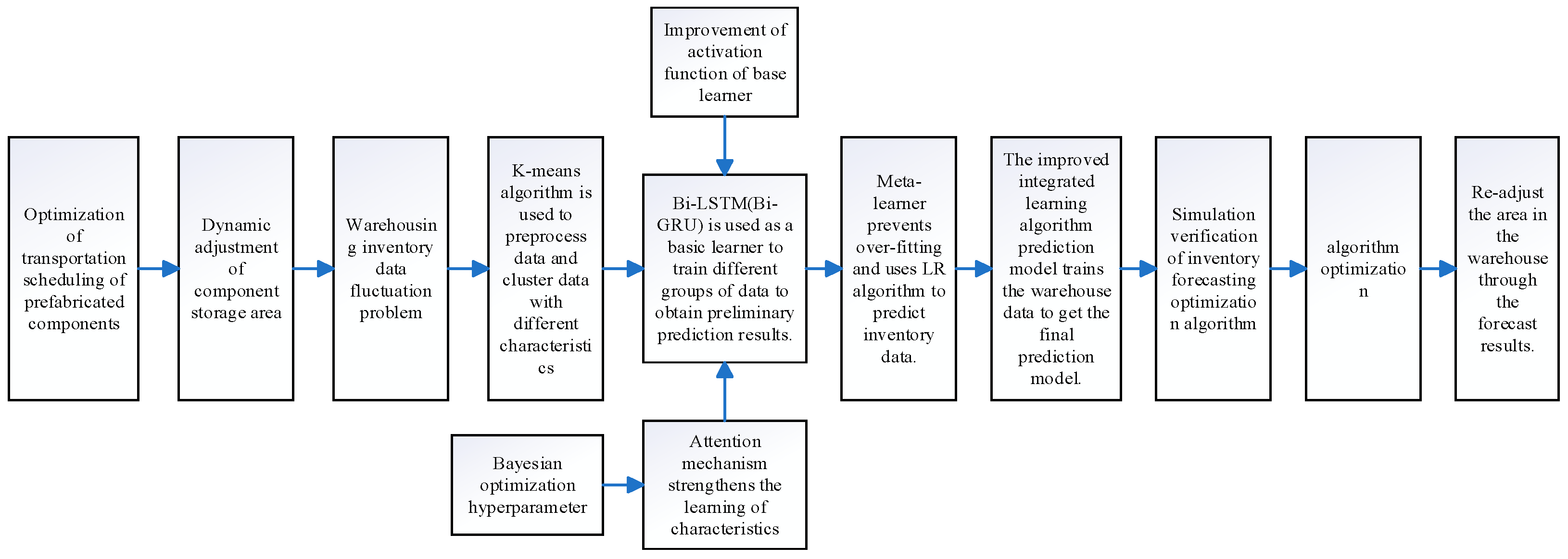
3. The Construction of an Ensemble Learning Model

The types of prefabricated components correspond directly to their respective storage areas. Therefore, by predicting the quantity of prefabricated components, necessary adjustments to the allocated storage area can be determined. To this end, we proposed a Stacking-based ensemble learning model for forecasting the number of prefabricated components, selecting an appropriate number of base learners based on data partitioning. Unlike traditional Stacking ensemble models—which utilize various base learners with different architectures to make predictions on the same dataset before combining outputs via a meta-learner—our approach adopts identical base learners but trains each on distinct subsets of the same dataset. This strategy enables the model to capture diverse feature sensitivities, allowing each base learner to specialize in specific feature patterns. As a result, these base learners can predict similar-feature data with improved efficiency compared to conventionally trained learners.

In our framework, Bi-LSTM with an integrated attention mechanism was initially selected as the base learner. Bayesian optimization was applied to fine-tune its hyperparameters, enhancing the model’s focus on salient data features and reducing training time. Given the large number of hyperparameters in the base learners, logistic regression (LR) was employed as the meta-learner in the second layer of the Stacking framework to prevent overfitting.

To further reduce computational time during training, Bi-LSTM was subsequently replaced by Bi-GRU. This modification led to a modest reduction in training duration without a significant compromise in predictive accuracy. Accordingly, the final ensemble learning model adopted Bi-GRU as the base learner. Technical roadmap is presented in Figure 1.

3.1. Long Short-Term Memory (LSTM) Network

As inventory fluctuation prediction is inherently a time series forecasting task, an LSTM network was employed for data analysis. Compared to classical Recurrent Neural Networks (RNNs), LSTM networks incorporate forget gates, input gates, and output gates, which collectively address the limitations associated with long-term information transmission—specifically, the loss of relevant historical data. Among these components, the forget gate plays a particularly critical role. It processes both the current input and the hidden state from the previous time step, outputting a value between 0 and 1 to determine the extent to which past information should be retained or discarded. This mechanism effectively mitigates issues related to vanishing and exploding gradients, enabling more stable and reliable training over long sequences. Figure 2 shows the LSTM structure diagram.

$$mis{h}^{*}=ax\times \tanh (\log {(1+e^x)}^r)$$

(1)

Replacing the traditional activation function with the improved Mish function yields a smoother activation curve, helping to alleviate issues such as gradient explosion and vanishing gradients. This enables the Mish function to better capture complex data patterns and relationships. Comparison between the improved Mish function and other activation functions can be observed in Figure 3.

3.2. Bidirectional Long Short-Term Memory (Bi-LSTM) Model

To address the limitations of traditional LSTM in inventory forecasting, particularly its inability to incorporate future information, a Bi-LSTM model was employed. By processing input sequences in both forward and backward directions, Bi-LSTM can capture contextual information from both past and future time steps. This bidirectional memory structure has demonstrated high predictive accuracy, especially when applied to highly stochastic and intermittent inventory data, making it well-suited for inventory stock forecasting tasks.

3.3. Bayesian Optimization

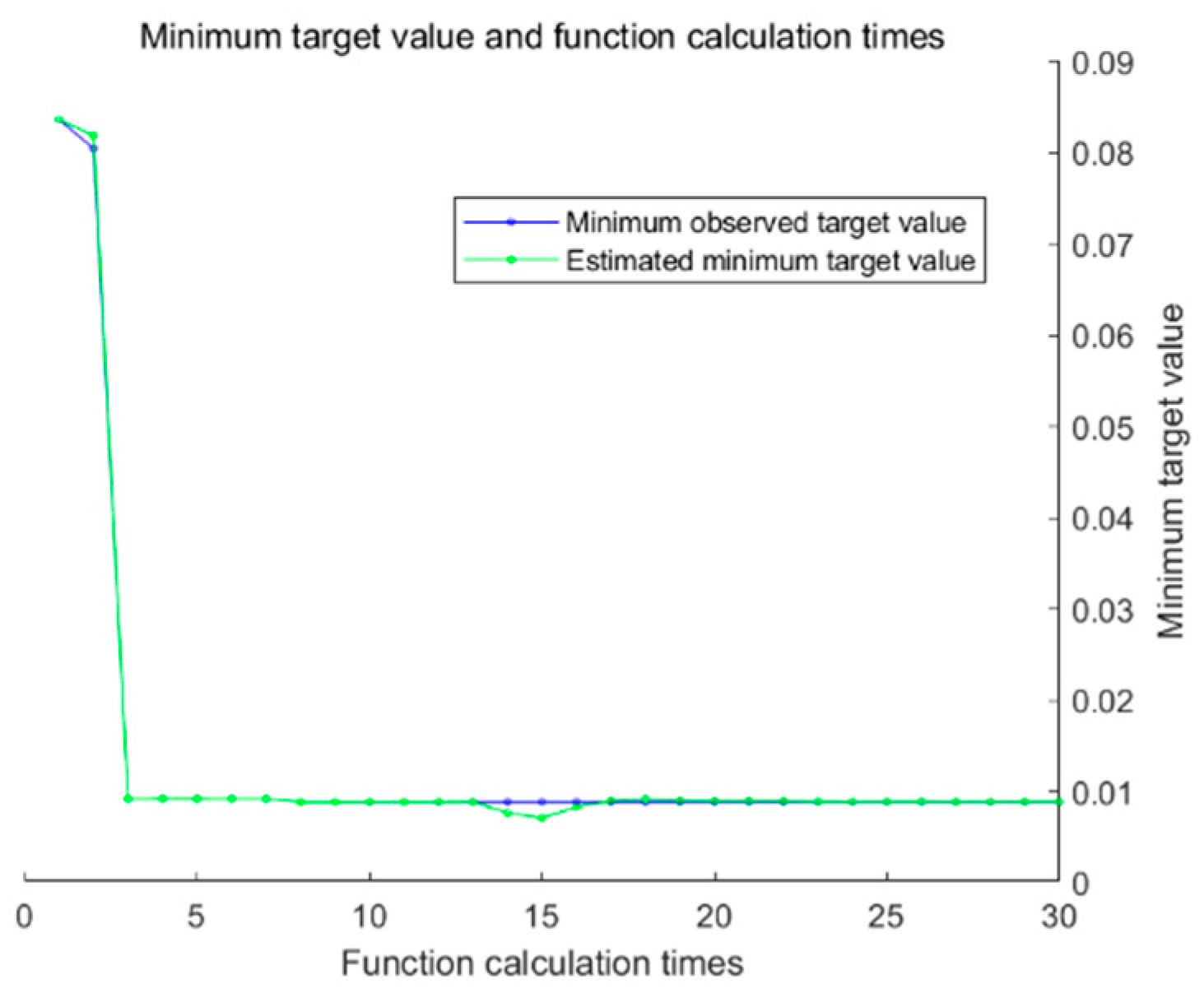
Bayesian optimization is a sequential optimization method based on probabilistic models, with its core principle centered on the “exploration-exploitation trade-off”. It constructs a probabilistic surrogate model of the objective function and strategically selects the next set of hyperparameters to evaluate by leveraging both the model and prior evaluation results. This approach allows for efficient convergence toward optimal solutions with minimal experimental runs, substantially reducing computational overhead. Compared to grid search and random search methods, Bayesian optimization minimizes inefficient sampling and typically identifies better-performing hyperparameters in fewer iterations—making it particularly suitable for deep learning models with long training times and large hyperparameter spaces. Given the numerous hyperparameters involved in our model, Bayesian optimization was employed to accelerate the training process and efficiently identify a well-performing network configuration. Bayes optimization flow chart can be observed in Figure 4.

3.4. K-Means Clustering

The fluctuation in inventory levels of prefabricated components is influenced by several factors, including the progress of component production and construction activities, which directly impact the quantity of inventory in storage. By employing the K-means clustering method, data points with similar influencing factors can be grouped, enabling more accurate predictions when training the model on clustered data.

Integrating K-means clustering with LSTM enhances the model’s effectiveness by exploring data from multiple dimensions. K-means categorizes data based on the similarity of influencing factors, while LSTM captures the correlation between these factors and the target variable, leading to improved prediction accuracy.

3.5. ABL Model

The improved LSTM algorithms, specifically the ATT-Bo-Bi-LSTM (ABL) model, were primarily used to extract information from input feature data. The attention mechanism aids in efficiently selecting key information from a vast array of features, focusing the model on the most relevant data for the task at hand. After passing through the Bi-LSTM, optimized through Bayesian methods and linked to the attention mechanism layer, the model filters out less impactful features. The refined feature information is then passed into a fully connected layer, where the results from the attention mechanism are aggregated to generate the final prediction.

3.6. ABG Model

The ABL model was replaced with the ATT-Bo-Bi-GRU (ABG) model to improve training speed. Bi-GRU, a variant of Bi-LSTM, simplifies the internal structure while retaining the effectiveness of Bi-LSTM in addressing time series problems. With fewer hyperparameters, Bi-GRU offers faster training compared to Bi-LSTM. Using ABG as the base learner in the ensemble learning model results in a significant increase in training speed, thus reducing the overall model training time.

3.7. Ensemble Learning Model

The effectiveness of a single model in inventory prediction is often limited, as it tends to focus on only one aspect of the data, frequently overlooking other important influencing factors. This can lead to inaccurate predictions or suboptimal model performance. To address these limitations, this paper proposes a multi-model overlay inventory prediction model based on ensemble learning. By employing the Stacking algorithm, various models’ predictions are combined, and predictions from single models serve as new training set data for secondary training, thereby enhancing the overall predictive capability of the model.

The Stacking prediction model is composed of two layers. The first layer consists of base learners, determined by clustering results. After training, the different prediction results from the base learners undergo weighted analysis and are input into a second-layer meta-learner, which generates the final prediction. This multi-model overlay inventory prediction model using the Stacking algorithm overcomes the bias and limitations associated with single models, improving overall predictive performance and robustness across various scenarios.

The ensemble learning model presented in this paper (LSTM–ensemble learning (LEL)) uses the ATT-Bo-Bi-LSTM (ABL) model as its base learner. The original data are clustered, and the resulting data groups are input separately into the base learners, ensuring their diversity and independence. Since using deep learning algorithms in the first layer may lead to overfitting, a simpler linear regression algorithm is chosen as the meta-learner in the second layer. This approach helps to minimize overfitting while controlling the overall complexity of the model. Striking a balance between avoiding overfitting and managing the model’s complexity is crucial. General flow chart can be observed in Figure 5.

In this study, the ABL model was replaced with the ATT-Bo-Bi-GRU (ABG), followed by retraining. Comparative experiments demonstrated that both ensemble learning models achieved comparable predictive accuracy. However, the ensemble learning model using ABG as its base learner (GRU–ensemble learning (GEL)) exhibited shorter training times than LEL. As a result, GEL is better suited for the real-time dynamic adjustments required in prefabricated component warehousing. Improved overall process flowchart can be observed in Figure 6.

4. Mathematical Model for Predicting Prefabricated Component Data

In the practical scheduling of prefabricated component warehousing, minimizing the time required for adjustments in the storage area is crucial for enhancing operational efficiency. Therefore, a mathematical model was developed to optimize the time needed for scheduling adjustments in prefabricated component warehousing.

The optimization model for precast component storage scheduling focuses on the prefabricated components that need to be adjusted, represented mathematically as follows:

$$\mathit{min}(\mathit{Mo}1-\mathit{Mo}2-\mathit{Mo}3)$$

(2)

Symbol and explanation can be observed in

Table 1. Symbol and explanation.

Symbol	Explanation
$\mathrm{Mo}1$	The sum of the maximum times for precast components during the storage scheduling process
$\mathrm{Mo}2$	The sum of the additional time incurred due to disordered component placement during precast component storage scheduling
$\mathrm{Mo}3$	The sum of the time spent on redividing areas during precast component storage scheduling
$M_i$	The average daily production quantity for each type of precast component by the manufacturing company
$N_i$	The daily average construction consumption quantity for each type of precast component
$T_k$	The current project’s storage area for precast components
$S_i$	The area occupied by each type of precast component
$T_{k+1}$	The new area
$S_{next}$	The adjusted area

. To optimize and adjust the current precast component storage area, the following steps were applied: the current working time period, denoted as $k$, was determined, and the in-stock and out-stock status of precast components for the next time period, $k+1$, were assessed.

$$S_{next}=T_{k+1}-T_k={\displaystyle \sum _{i\in (1,2\dots n)}^i(M_i-N_i)}\times S_i$$

(3)

Various influencing factors were set as follows: $C_q$, $q$$\in$(1, 2 …n).

Let us assume there are n types of prefabricated components transported to m different project storage areas. $O$ is the set of prefabricated components, $O\in \left(1,2\dots n\right)$, where $\mathrm{i}$ is the index of the type of prefabricated component, $\mathrm{i}\in O$, and $j$ is the storage area number for storing these prefabricated components, $j\in (1,2\dots m)$. If prefabricated component $\mathrm{i}$ is stored in area $j$, then $x_{ij}$ is 1; otherwise, it is 0. For the prefabricated component i, the scheduling time for warehousing transfer to area $j$ is represented as $r_{ij}$, and the time consumed for warehousing search in the area is represented as $c_{ij}$. $w$ represents the influencing factor that leads to the number of prefabricated components in the warehouse. $d_i$ represents the time required for re-planning the consumption of prefabricated component $\mathrm{i}$ in the warehouse.

Based on the information provided above, the problem of dynamic adjustment of prefabricated component storage area can be described as follows $\mathit{min}(\mathit{Mo}1-\mathit{Mo}2-\mathit{Mo}3)$; the specific objective function can be formulated as follows:

$$Min({\lambda }_1{\displaystyle \sum _{i=1}^n{\displaystyle \sum _{j=1}^m{x}_{ij}{r}_{ij}-}}{\lambda }_2{\displaystyle \sum _{i=1}^n{\displaystyle \sum _{j=1}^m{x}_{ij}{c}_{ij}-{\lambda }_3{\displaystyle \sum w{d}_i}}})$$

(4)

In the objective function model, the first term ${\lambda }_1{\displaystyle \sum _{i=1}^n{\displaystyle \sum _{j=1}^m{x}_{ij}{r}_{ij}}}$ ensures the total time spent on the storage scheduling of each prefabricated component in the warehouse, aiming to maximize the rational utilization of each project area. The second term ${\lambda }_2{\displaystyle \sum _{i=1}^n{\displaystyle \sum _{j=1}^m{x}_{ij}{c}_{ij}}}$ represents the total time spent on searching for storage areas for prefabricated components, aiming to minimize search time operations. The third term ${\lambda }_3{\displaystyle \sum w{d}_i}$ accounts for the time spent on reassigning storage areas during the transportation process, ensuring that the scheduling proceeds according to the plan, where ${\lambda }_i,i\in (1,2\dots n)$ represents the weights of the objective function terms, ${\displaystyle {\sum }_i{\lambda }_i}$. The constraints are as follows:

(1)

The constraints ensure that each prefabricated component is stored in its corresponding project area, and each project area has one and only one:

$${\displaystyle \sum _{j=1}^m{x}_{ij}}\le 1,i=1,2\dots n,j=1,2\dots m$$

(5)

(2)

Ensure that the production rate is more than the consumption rate when the decrease in the number of prefabricated components is caused by external factors:

$${\displaystyle \sum _{i=1}{d}_i{N}_i}<{\displaystyle \sum _{i=1}{d}_i{M}_i},i=1,2\dots n$$

(6)

(3)

Ensure that the adjusted storage area for prefabricated components is more than the sum of the areas of all prefabricated components within the region:

$${\displaystyle \sum _{i=1}^n{\displaystyle \sum _{j=1}^m{x}_{ij}{S}_i\le {\displaystyle \sum _{j=1}^m{\displaystyle \sum _{k=1}{T}_{k+1}{x}_{ij},i=1,2\dots n,j=1,2\dots m}}}}$$

(7)

(4)

Ensure that the total time during the dynamic partitioning of storage areas is more than the optimization time:

$${\displaystyle \sum _{i=1}^n{\displaystyle \sum _{j=1}^m{x}_{ij}{r}_{ij}\ge }}{\displaystyle \sum _{i=1}^n{\displaystyle \sum _{j=1}^m{x}_{ij}{c}_{ij}}}+{\displaystyle \sum w{d}_i}$$

(8)

Use the K-means algorithm to cluster the original data into groups, resulting in $G_1,G_2\dots G_n$. Split the clustered data into a 70% training set $D_{train}$ and a 30% test set $D_{test}$. Input $G_1,G_2\dots G_n$ to the ATT-Bo-Bi-LSTM model separately for training, resulting in n base learners. To improve the model’s generalization ability and avoid the situation where the model performs well on known data but poorly on unknown data, 5-fold cross-validation is used during training. The training set is divided into $D_{train}^1$, $D_{train}^2$, $D_{train}^3$, $D_{train}^4$, and $D_{train}^5$. In sequence, with each portion serving as the validation set for five iterations of training. The trained model equation is as follows:

$$M_i^k=N_i(D_{train}-D_{train}^k)$$

(9)

where $M_i^k$ represents the model obtained by the i-th algorithm in the k-th cross-validation training, and $N_i$ represents the i-th algorithm:

$${\stackrel{\wedge }{Y}}_i^k=M_i^k(D_{train}^k)$$

(10)

$${\stackrel{\wedge }{Y}}_i=({\stackrel{\wedge }{Y}}_k^1,{\stackrel{\wedge }{Y}}_k^2,{\stackrel{\wedge }{Y}}_k^3,{\stackrel{\wedge }{Y}}_k^4,{\stackrel{\wedge }{Y}}_k^5)$$

(11)

where ${\stackrel{\wedge }{Y}}_i^k$ represents the predictions made by the i-th base learner on the validation set $D_{train}^k$ during the k-th cross-validation iteration, and ${\stackrel{\wedge }{Y}}_i$ represents the predictions made by the i-th base regressor on the n samples from all the validation sets $D_{train}^k$ after the 5-fold cross-validation.

$${\stackrel{\wedge }{Z}}_k^i=M_i^k(D_{test})$$

(12)

$${\stackrel{\wedge }{Z}}_i={\displaystyle \frac{1}{5}}{\displaystyle \sum _{k=1}^5{\stackrel{\wedge }{Z}}_k^i}$$

(13)

where ${\stackrel{\wedge }{Z}}_k^i$ represents the predictions made by the i-th base learner on the test set $D_{test}$ using the base learner $M_i^k$ during the k-th cross-validation iteration, and ${\stackrel{\wedge }{Z}}_i$ represents the average of all the predictions made by the i-th base learner during cross-validation.

In the second-layer linear regression model, a new training set $S_{train}$ and a new testing set $S_{test}$ are constructed using the results from the first-layer base learners. The predictions are then made based on these new sets:

$$M_{stacking}=LR(S_{train})$$

(14)

$$\mathit{Pre}Sets=M_{stacking}(S_{test})$$

(15)

$$\mathit{Pre}Se{t}_D=M_{stacking}(D_{test})$$

(16)

where $D_{test}$ is input into the $M_{stacking}$ model to validate the accuracy of the model.

The initial area for component storage is $S_{origin}$, and the number of components in the current stage in the area is $N_{origin}$. The area for the next stage is adjusted to $S_{next}$.

$$S_{next}={\displaystyle \frac{S_{origin}}{N_{origin}}}\mathit{Pre}Se{t}_D$$

(17)

5. Experimental Simulation Comparison

The previous management and information system for stacking prefabricated components was inadequate, resulting in incomplete historical data. In recent years, with the advancement of informatization, the information system has been better managed. However, the dataset for prefabricated components remains relatively small. To validate the effectiveness of our method, we selected the Chinese port container throughput dataset, as it shares similarities with our prefabricated component data. Both involve large-volume items, making the port dataset suitable for our validation purposes.

Therefore, transportation scheduling data from port container logistics, which closely resembles the structure of prefabricated component transportation and scheduling, was utilized for training. Over time, the scheduling data will be enhanced in collaboration with prefabricated component production companies. The proposed model will then be retrained using the prefabricated component dataset. To demonstrate the effectiveness of the proposed dynamic prediction method for prefabricated component storage, a simulation experiment environment was set up for validation. The validation was conducted on a system with an Intel Core i5-8300H processor, Windows 10 OS, and 16 GB of memory. All experiments in this study were carried out using Python 3.8, with analyses performed on PyCharm 2019.

5.1. Data Preprocessing

This paper utilized the Chinese port container throughput data for model training. Seven factors influencing container storage fluctuations—container outbound volume, berth capacity, container inbound volume, current container storage volume, container cargo type, vessel transport time to the site, and container inspection results—were used as inputs. These factors were grouped using the K-means algorithm. As shown in Figure 7, the initial K value is randomly defined, and the variance ratio criterion (Calinski-Harabasz, CH) is used to assess the reasonableness of the K value. The K value is adjusted until the CH index approximates 1. The K value closest to 1 is then determined as the optimal number of clusters.

The CH evaluation index concludes that the optimal number of clusters is 3, with the CH index being closest to 1. Therefore, the current influencing factors are categorized into three groups according to the CH index, and the clustering results are visualized as shown in Figure 8. As a result, the overall data are divided into three clusters.

5.2. Comparison Between ABL and Unimproved LSTM Prediction

A Bo-Bi-LSTM neural network prediction algorithm was developed, incorporating an attention mechanism. The overall model consists of an input layer, a Bi-LSTM layer, an attention mechanism layer, a fully connected layer, and an output layer. Bayesian optimization is used as the learning algorithm for the Bi-LSTM network. Unlike traditional hyperparameter optimization methods, Bayesian optimization can automatically adjust the learning rate for weights. Compared to the classic LSTM network, this approach allows for the quicker identification of suitable hyperparameters, facilitating the convergence of the short-term prediction model. Additionally, it helps avoid the issue of the model getting stuck in local optima during training. The model was trained for a total of 1000 iterations.

Based on the Bayesian optimization algorithm for hyperparameter tuning, and after iterative evaluations of the objective function,

Table 2. Optimized hyperparameter values of LSTM neural network.

Parameter	Value	Parameter	Value
LSTM layer	2	Error parameter	MSE
LSTM layer Number of neurons	128	L2 regularization parameter	0.0001
Probability of discarding neurons	0.3	Learning rate	0.016
Ergodic times	1000	Time step	15
Standardization rule	Minimization–maximization (0,1)	Training time window	24

presents the hyperparameter combination that resulted in the minimum loss of the objective function. The optimized hyperparameter values are as follows (see Table 2): number of neurons = 128; learning rate = 0.016; dropout probability = 0.3; L2 regularization = 0.0001; training time window = 24. To balance convergence speed and computational efficiency, the maximum number of iterations is set at 1000, a value that has been experimentally validated in the previous literature for effective error convergence.

Figure 9 and Figure 10 show the comparison of the prediction curves between the ABL model proposed in this paper and the classic LSTM using the same dataset. From the comparison of these two sets of images, it can be observed that the predicted values from the ABL model align more closely with the actual values, indicating that the ABL model performs better than the LSTM model in predicting time series data. Bayesian optimization process chart is shown as Figure 11.

5.3. Comparison Between the LEL Model and Single ABL Model

This paper uses the Stacking ensemble learning model. During training, each base learner was trained using a 5-fold cross-validation method. This approach divides the training set into five equal parts, iteratively using each part as the validation set across five iterations. The predictions from these five iterations on the validation set are used as the training set for the second layer, while the test set results from the base learners are used as the test set for the second layer. Finally, a logistic regression (LR) algorithm serves as the meta-learner to train and obtain the final prediction results.

Figure 12 and Figure 13 show the comparison of the prediction curves between the LEL ensemble learning model proposed in this paper and the single ABL model using the same dataset. From the figures, it is evident that the ensemble learning model offers better prediction accuracy than the single model.

5.4. Indicators for the Evaluation of Predictive Models

To evaluate the performance of the models, this study employs several evaluation metrics to assess the effectiveness of the short-term prediction model. These metrics include the mean absolute error (MAE), coefficient of determination (R²), root mean square error (RMSE), and mean absolute percentage error (MAPE). The mathematical expressions for these metrics are shown in Equations (15)–(18).

$$MAE={\displaystyle \frac{{\displaystyle \sum _{g=1}^{n_0}|{\stackrel{\wedge }{y}}_g-y_g|}}{n_0}}$$

(18)

$$R^2=1-{\displaystyle \frac{{\displaystyle \sum _i{({\stackrel{\wedge }{y}}_i-y_i)}^2}}{{\displaystyle \sum _i{({\stackrel{=}{y}}_i-y_i)}^2}}}$$

(19)

$$RMES=\sqrt{{\displaystyle \frac{{\displaystyle \sum _{g=1}^{n_0}{({\stackrel{\wedge }{y}}_i-y_i)}^2}}{n_0}}}$$

(20)

$$MAPE={\displaystyle \frac{1}{n_0}}{\displaystyle \sum _{g=1}^{n_0}\frac{|{\stackrel{\wedge }{y}}_g-y_g|}{{\stackrel{\wedge }{y}}_g}}$$

(21)

5.5. Experimental Comparison

To evaluate the short-term prediction performance and robustness of the model, an experiment was conducted comparing various models, including the classical LSTM network, bidirectional LSTM network, BP neural network, gray prediction model, and ABL. To demonstrate the effectiveness of the ensemble learning model, comparisons were made between the model without ensemble learning (ABL) and the ensemble learning model proposed in this paper (LSTM–ensemble learning (LEL)). The evaluation metrics are presented in

Table 3. Comparison diagram of methods.

Method	RMES	MAE	MAPE	R2	Growth Rate
BP	2.4965	2.1654	0.1751	0.9537	+0.26%
GM	2.2507	1.7198	0.1396	0.9512	0%
LSTM	2.5897	2.1833	0.1851	0.9572	+0.63%
Bi-LSTM	1.5852	1.3759	0.1083	0.9608	+1.01%
ABL	1.1323	0.9924	0.0769	0.9626	+1.20%
LEL	1.0773	0.6245	0.0443	0.9834	+3.38%

. The graph illustrates the mean absolute percentage error results from the table, providing a more intuitive comparison.

When comparing the predictive accuracy of different models, the R² value of the poorest-performing GM model was used as a benchmark. The improvement percentage of other models was calculated by subtracting the benchmark value from the evaluated value, obtaining the absolute difference, dividing this difference by the benchmark value, and then multiplying by 100% to express the result as a percentage. This percentage reflects the improvement of the evaluated model over the benchmark.

The results showed that the LEL model exhibited an improvement of 3.38%, significantly outperforming the other comparative models. This demonstrates that the LEL model is more effective and better suited for predicting the quantity of prefabricated components.

Ablation experiments were conducted on the ABL model to verify its superior predictive performance. Additionally, to validate the faster training speed of ABG, a comparative analysis of the training times between ABG and ABL was performed.

From

Table 4. Sensitivity analysis experiment.

Method	RMES	MAE	MAPE	R2	Training Time t/s
LSTM	2.5897	2.1833	0.1851	0.9572	133.65
Bi-LSTM	1.5852	1.3759	0.1083	0.9608	274.12
Bo-Bi-LSTM	1.4755	1.1294	0.0812	0.9614	243.25
ABL	1.1323	0.9924	0.0769	0.9626	302.46
ABG	1.1331	0.9875	0.0763	0.9640	298.45

, it can be concluded that both ABL and ABG perform better in forecasting time series data, with the evaluation index for ABL showing improvement compared to its original model. Compared to the ABL model, ABG reduced the training time by 1.3%, indicating that ABG offers faster training speed.

Figure 14 illustrates the forecast results from traditional models, such as BP neural networks, alongside the proposed ensemble learning model applied to the same dataset.

The x-axis represents months, while the y-axis represents the number of containers. The green curve in Figure 14 represents the LEL ensemble learning model proposed in this paper, and the red curve represents the true values from the dataset.

Other curves represent predicted values from various models. As seen in the figure, the green LEL curve exhibits the highest degree of alignment with the true value curve, while the other curves show considerable deviations at different time points. This demonstrates that the LEL model proposed in this study achieves higher accuracy.

5.6. Algorithm Improvement Based on Training Time

During the experimentation, it was observed that LSTM requires a longer training time due to the large number of hyperparameters. To expedite the process and obtain predictions more rapidly, LSTM was replaced with GRU. Unlike LSTM, GRU maintains similar functionality but has a simpler structure and fewer hyperparameters.

The ABG model proposed in this paper is compared with the Stack-XGBoost ensemble learning model introduced in reference [29]. Optimized hyperparameter values for GRU neural network is shown as

Table 5. Optimized hyperparameter values for GRU neural network.

Parameter	Value	Parameter	Value
GRU layer	2	Error parameter	MSE
GRU layer number of neurons	256	L2 regularization parameter	0.0001
Probability of discarding neurons	0.25	Learning rate	0.005
Ergodic times	1000	Time step	15
Standardization rule	Minimization–maximization (0,1)	Training time window	24

.

From

Table 6. Evaluation index of different ensemble learning models.

Method	Ensemble Models	Base Learners	MAPE	R2	RMES	MAE
1	AdaBoost	ABL	0.0984	0.9696	1.1033	0.8575
2	Stack-XGBoost	ETR and RFR AdaBoost	0.0422	0.9845	1.0765	0.6134
3	LEL	ABL	0.0443	0.9834	1.0773	0.6345
4	GEL	ABG	0.0436	0.9836	1.0769	0.6179

and

Table 7. Training data and memory occupation of different ensemble learning models.

Method	Ensemble Models	Base Learners	Training Time t/s	Memory Usage/MB
1	AdaBoost	ABL	643.44	657
2	Stack-XGBoost	ETR and RFR AdaBoost	610.56	1045
3	LEL	ABL	601.25	564
4	GEL	ABG	587.58	529

, it can be observed that LEL and GRU–ensemble learning (GEL) exhibit similar performance across various evaluation metrics. However, GEL shows a 2.32% faster training time than LEL and a reduction in memory usage by 6.61%. Compared to the Stack-XGBoost ensemble learning model, although GEL’s performance on some evaluation metrics is slightly inferior, it excels in training time and memory utilization.

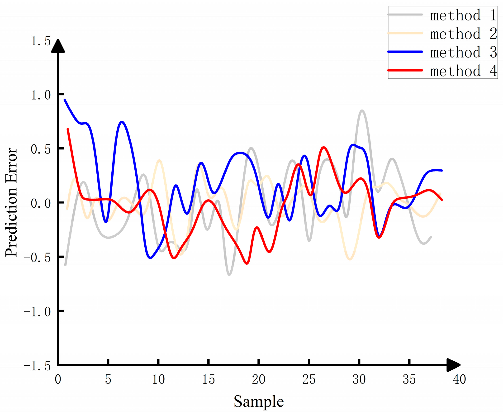
As shown in Figure 15, Methods 3 and 4 exhibit more stable errors compared to the ensemble learning model of Method 1. Method 3 shows 14 instances with absolute errors exceeding 5%, constituting 7% of the total samples, while Method 4 exhibits 12 instances with absolute errors exceeding 5%, accounting for 6% of the total samples. Only one instance in Method 4 exceeds 10% in absolute error. Method 1 shows a quantity of errors exceeding 10%, which is 1.42 times greater than Methods 3 and 4. Therefore, it can be concluded that Methods 3 and 4 demonstrate better data analysis and prediction capabilities than Method 1, showcasing higher stability.

Method 2 outperforms the proposed method in various prediction indicators and performs better in predicting data than Methods 3 and 4. However, according to Table 7, Methods 3 and 4 excel in terms of model training time and memory usage. In particular, Method 4 shows advantages in training time and memory utilization. In summary, the proposed dynamic prediction method for prefabricated component storage areas applies to various samples, providing more accurate predictions than typical ensemble learning models, demonstrating smoother prediction errors, and showcasing higher reliability and stability.

In conclusion, by designing comparative experiments, it can be observed that the ensemble model proposed in this paper has stronger general applicability, certain advantages in various indicators, and high reliability and stability. Due to the limited data on prefabricated component storage currently available, this paper uses similar datasets for training. The model’s performance would improve with more comprehensive long-term data. Additionally, better hardware configurations would also enhance the results.

6. Conclusions

Planning prefabricated component storage areas is crucial for component production planning and construction schedule management. This paper focuses on the dynamic adjustment of prefabricated component inventory storage areas. The comparison of the improved ensemble learning model’s prediction curve with other classic prediction models demonstrates a higher degree of overlap between the improved ensemble learning model and the real value curve. The GEL model is proposed to enhance model training speed, showing a 2.32% improvement in training speed compared to the LEL model. Compared to LEL, AdaBoost, and Stack-XGBoost algorithms or models, GEL exhibits reduced error fluctuations and improved prediction accuracy. Notably, GEL also shows more efficient training time and memory usage than Stack-XGBoost.

This study is particularly suited for real-time adjustments in prefabricated component storage areas. It confirms that the improved ensemble learning model is more accurate in forecasting than single models. This approach can be applied to real-time inventory management systems in enterprises, integrated with other management systems to optimize production plans. Ultimately, we aim to build an Internet-plus-cloud platform for the industrial Internet, deeply integrating production and management processes. This platform will enhance coordination between inventory forecasting models and the entire enterprise production control system. In the future, it could be combined with large language models to further improve adaptability to production and operational changes and enhance the ability to handle unexpected situations, thereby improving prediction accuracy.