
Solar Radiation Prediction Based on the Sparrow Search Algorithm, Convolutional Neural Networks, and Long Short-Term Memory Networks


Abstract
1. Introduction
2. Methodology
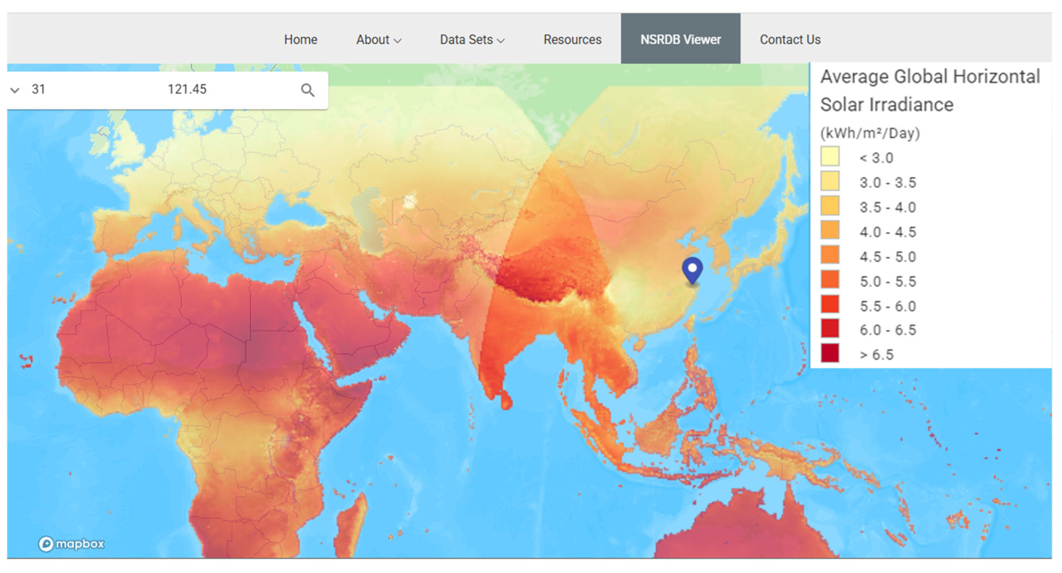
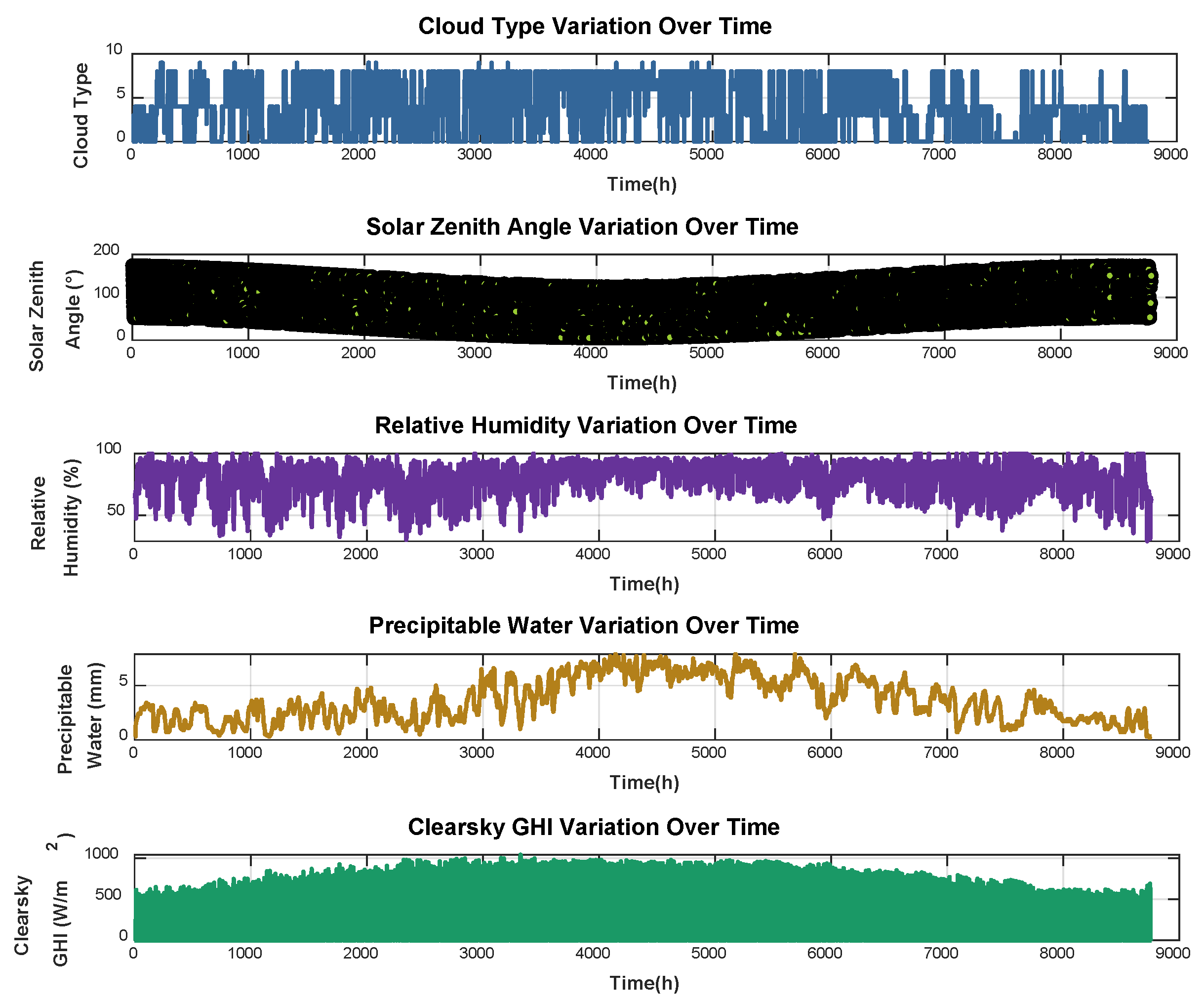
2.1. Data Collection
2.2. Data Preprocessing
2.3. Deep Learning Models
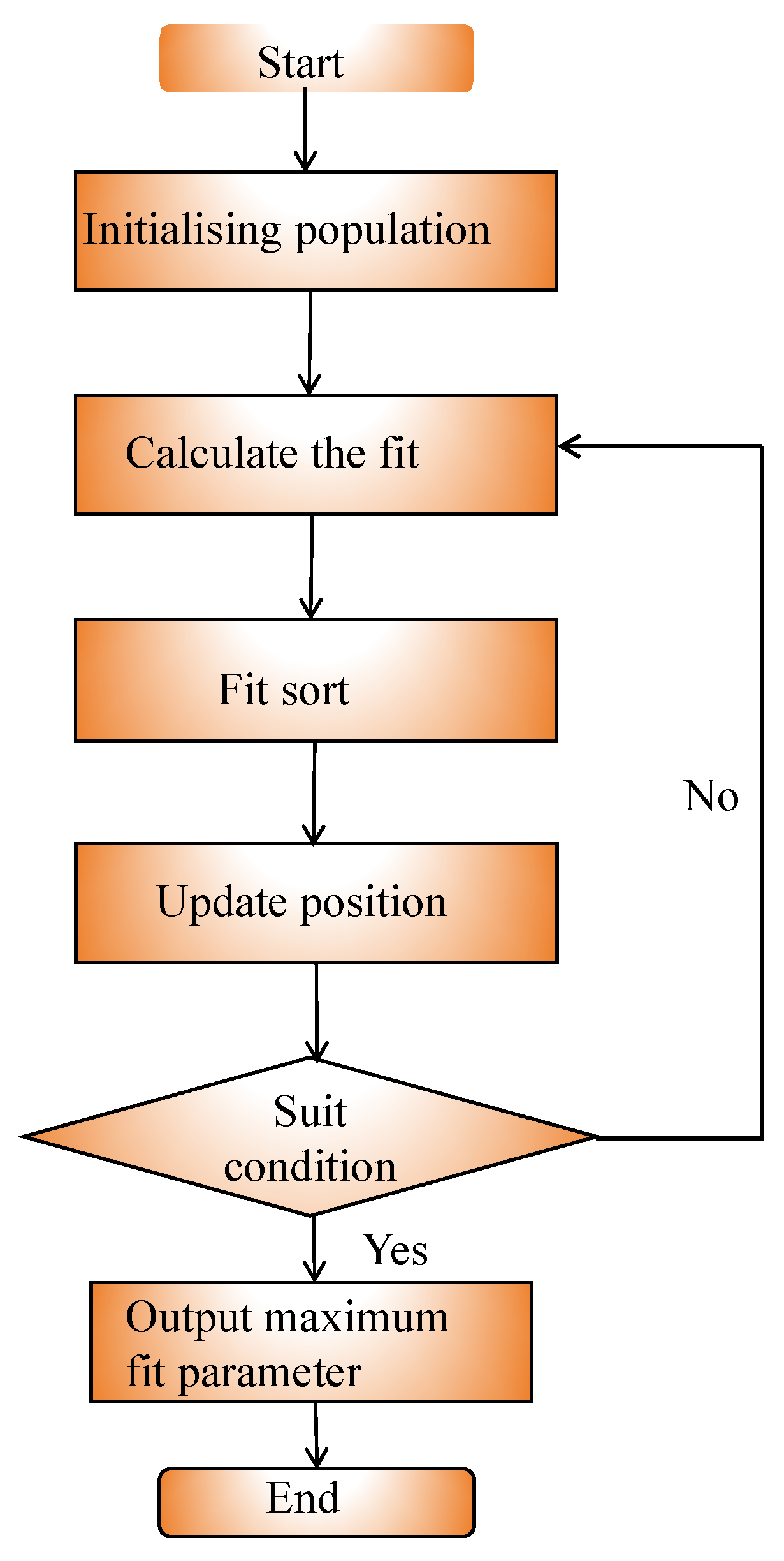
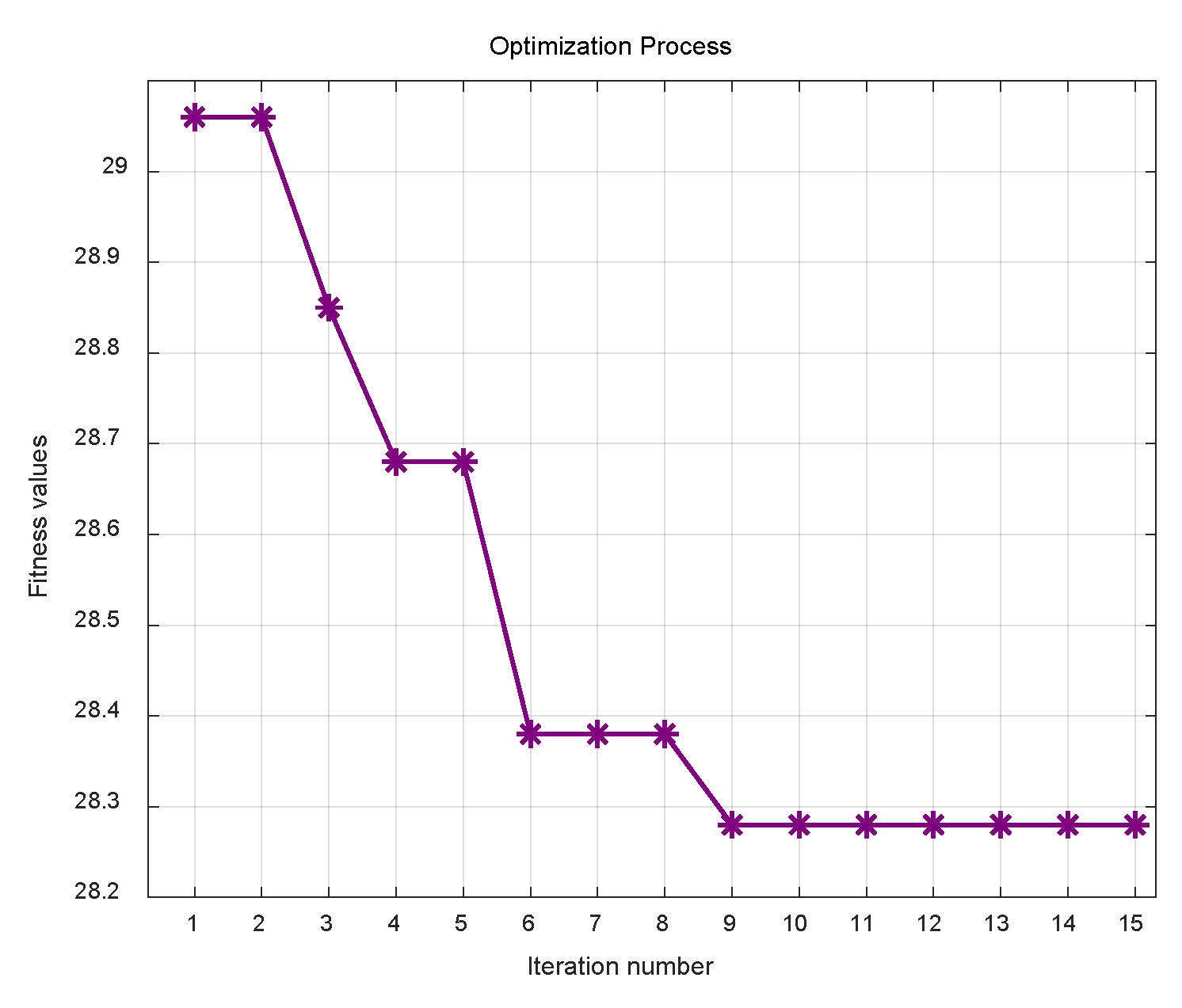
2.3.1. Sparrow Search Algorithm (SSA)
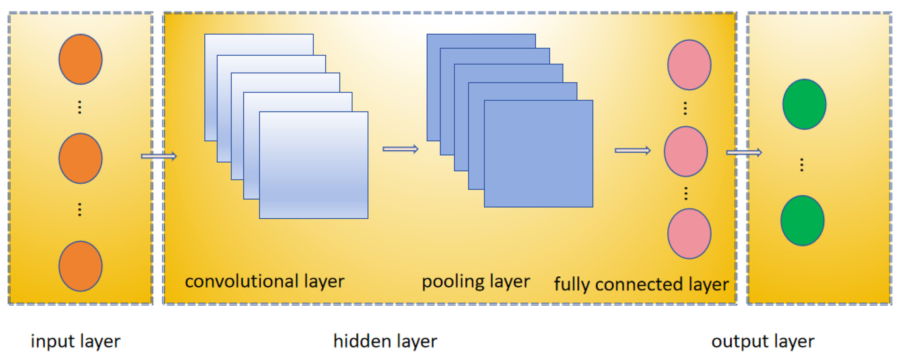
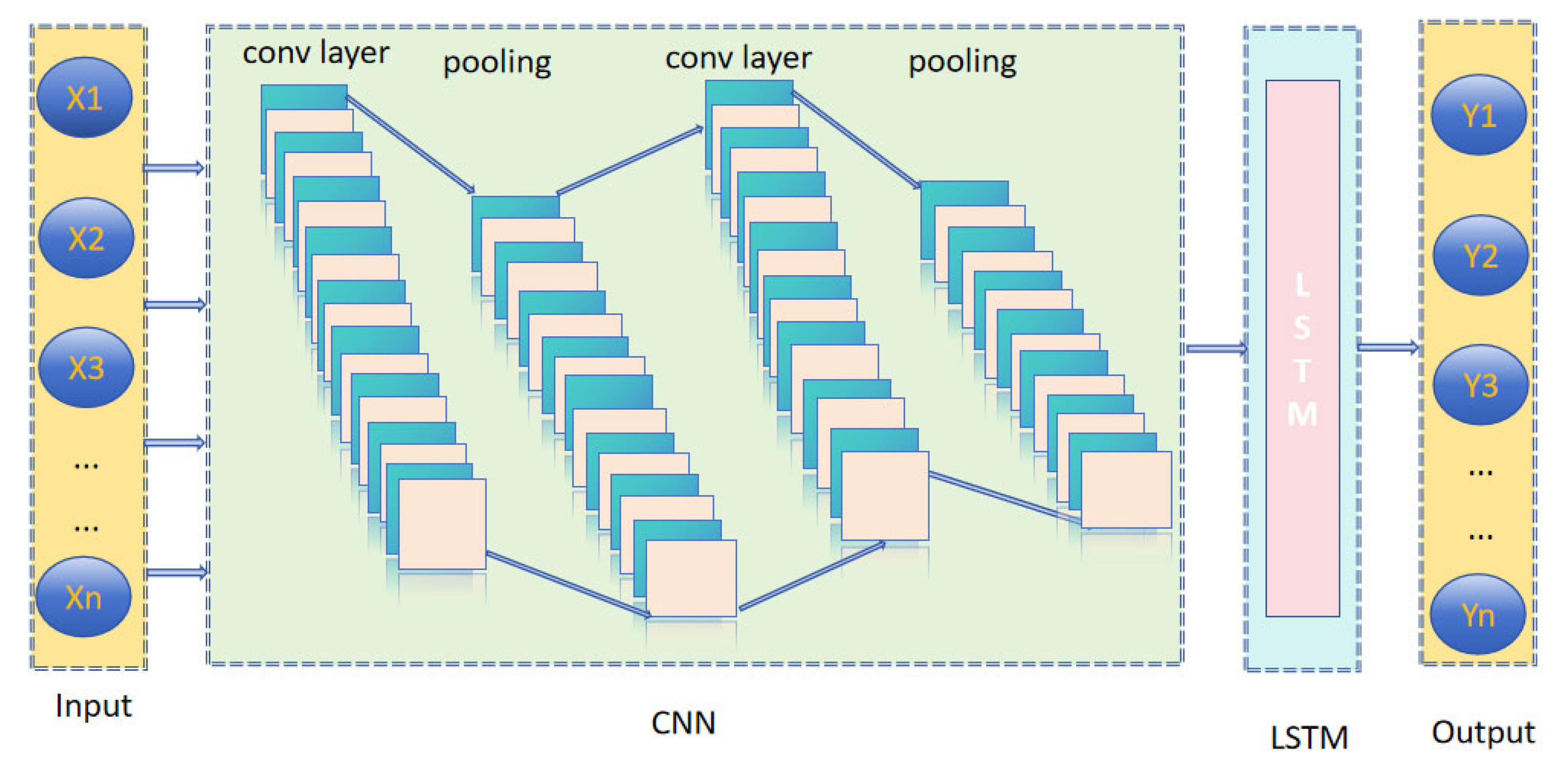
2.3.2. Convolutional Neural Network (CNN)
2.3.3. Long- and Short-Term Memory (LSTM)
2.3.4. CNN-LSTM
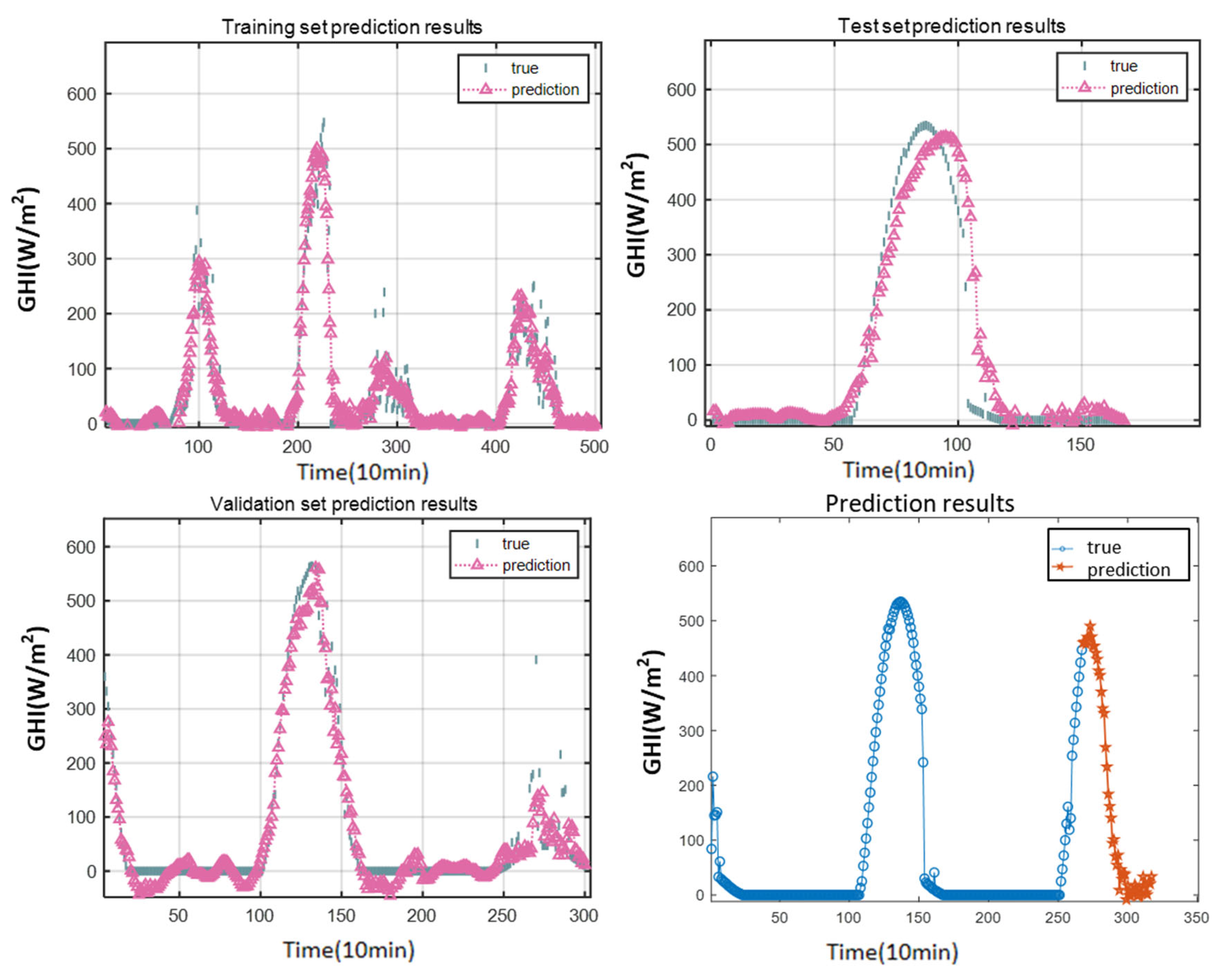
2.3.5. SSA-CNN-LSTM
2.4. Model Evaluation
2.4.1. Mean Absolute Error (MAE)
2.4.2. Root Mean Square Error (RMSE)
2.4.3. Coefficient of Determination
3. Results and Discussion
3.1. Results
3.1.1. Model Parametric and Experimental Environment
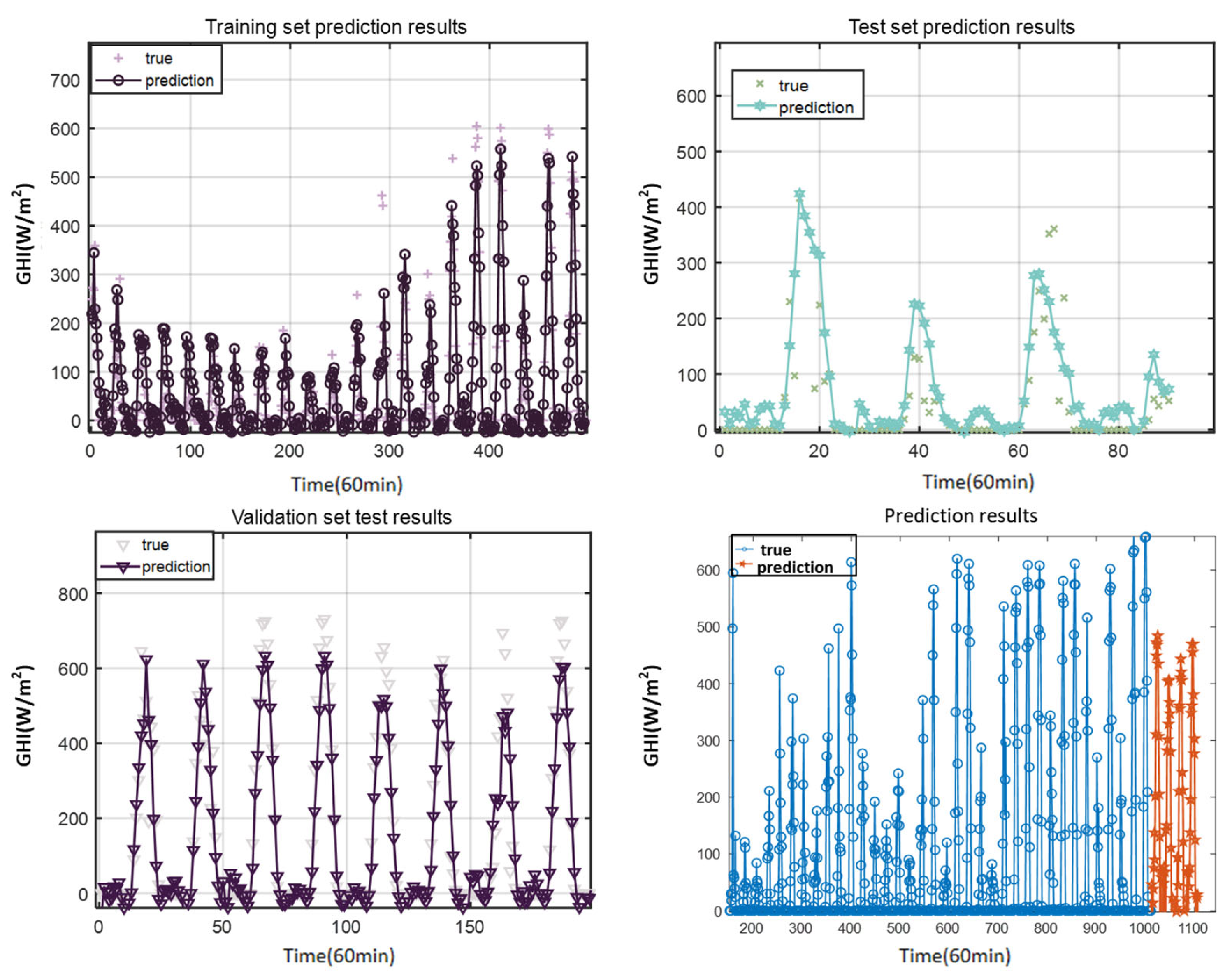
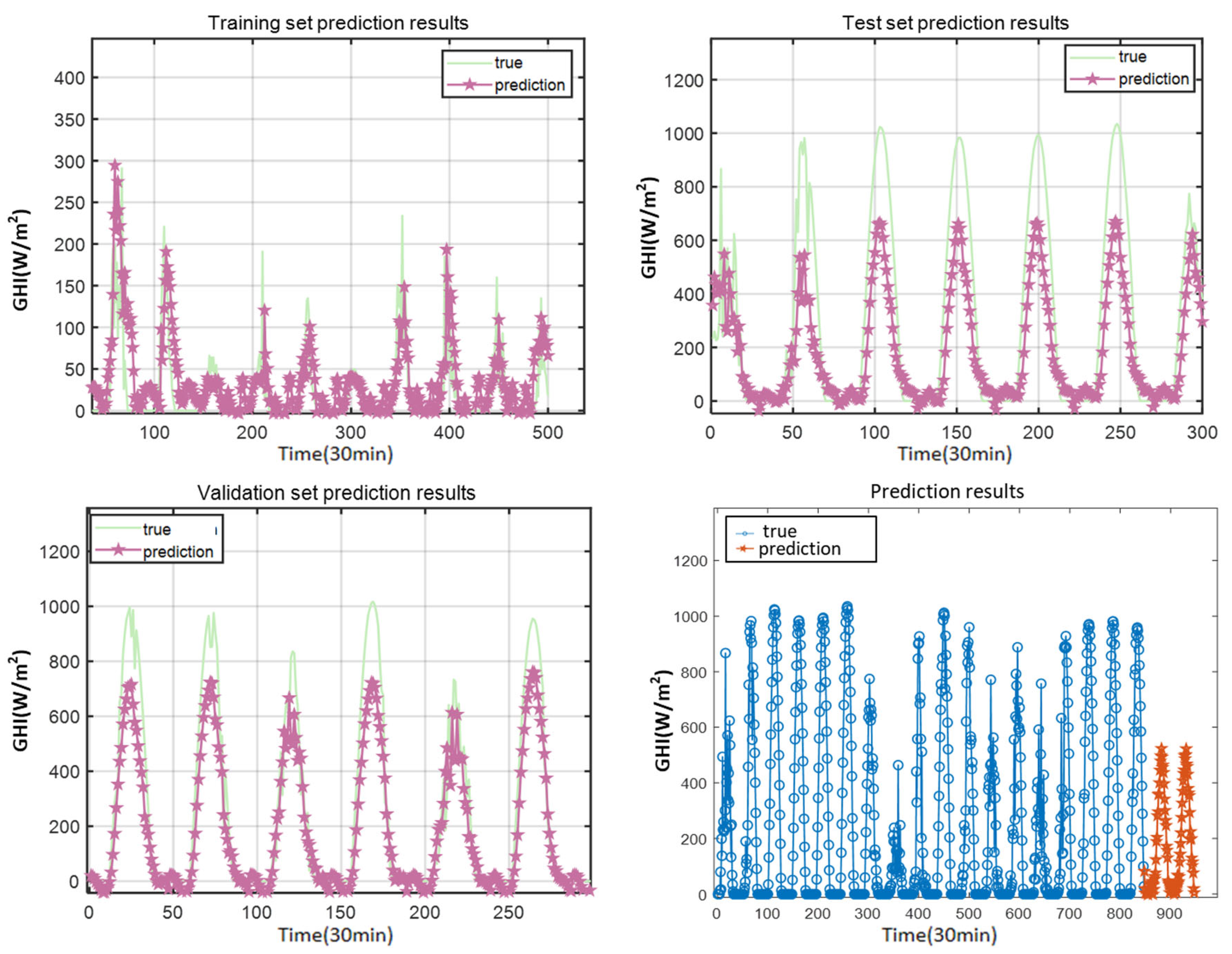
3.1.2. Results of the Experiment
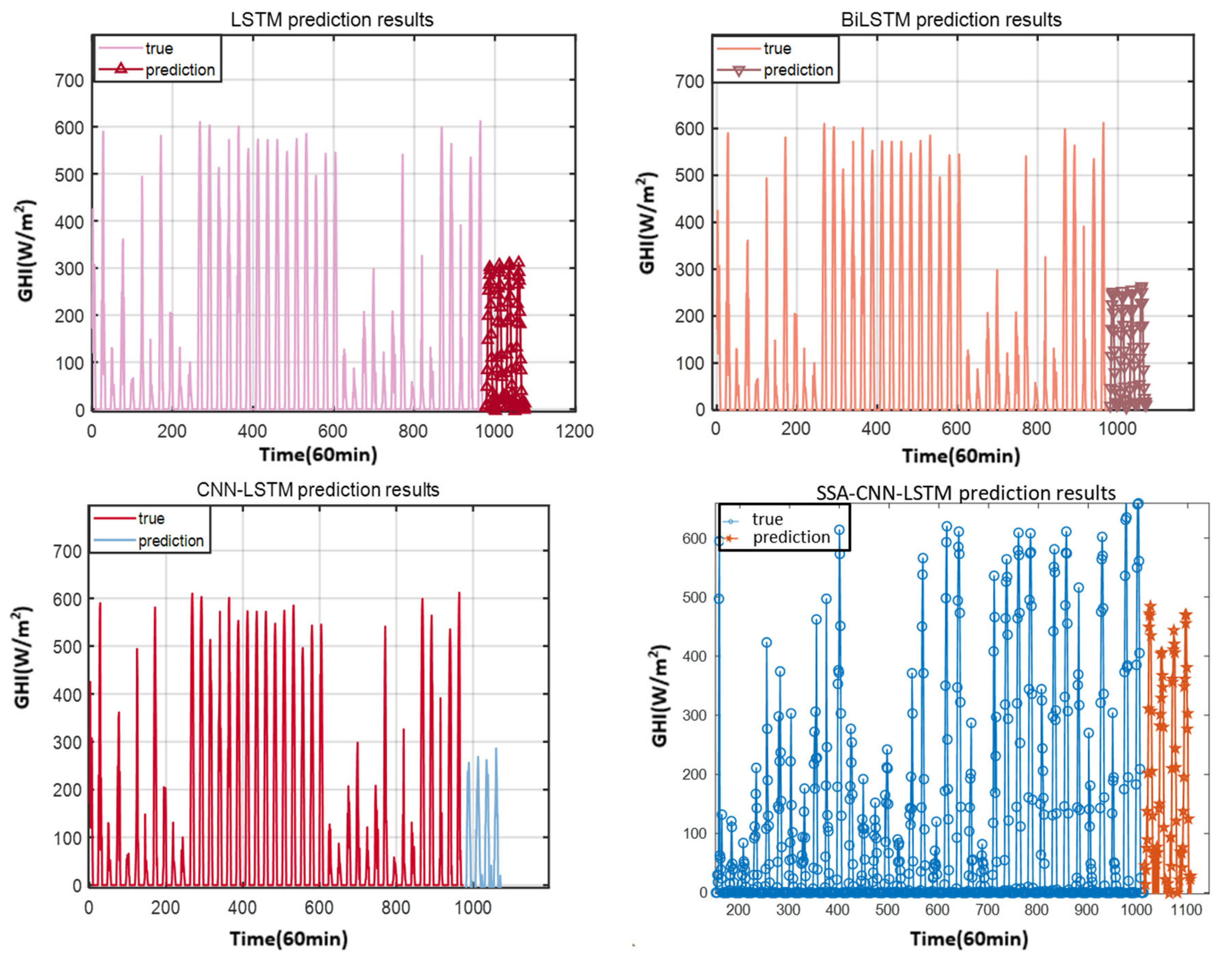
3.1.3. Comparison Experiment
3.2. Discussion
4. Conclusions
Author Contributions
Funding
Data Availability Statement
Conflicts of Interest
Nomenclature
| SSA | Sparrow Search Algorithm |
| CNN | Convolutional Neural Networks |
| LSTM | Long Short-Term Memory Networks |
| NSRDB | National Solar Radiation Database |
| GHI | Global Horizontal Irradiance |
| EM | Expectation Maximization |
| ARIMA | Auto-Regressive Integrated Moving Average |
| AGA | Adaptive Genetic Algorithm |
| RF | Random Forest |
| SVR | Support Vector Regression |
| GBM | Gradient Boosting Machine |
| ANN | Artificial Neural Network |
| SOM-OPEM | Self-Organizing Map-Optimal Path Extraction Method |
| MAE | Mean Absolute Error |
| RMSE | Root Mean Square Error |
References
- International Energy Agency. CO2 Emissions in 2023. 2023. Available online: https://www.iea.org/reports/co2-emissions-in-2023 (accessed on 5 December 2024).
- Herrando, M.; Markides, C.N.; Hellgardt, K. A UK-based assessment of hybrid PV and solar-thermal systems for domestic heating and power: System performance. Appl. Energy 2014, 122, 288–309. [Google Scholar] [CrossRef]
- Röhrig, P.M.; Martens, J.; Körber, N.; Kurth, M.; Ulbig, A. Analysis of PVT hybrid roof-top systems for the energy supply of electricity and heat for buildings. In Proceedings of the IEEE PES Innovative Smart Grid Technologies Conference Europe, Grenoble, France, 23–26 October 2023; p. 10407104. [Google Scholar]
- Naghdbishi, A.; Yazdi, M.E.; Akbari, G. Experimental investigation of the effect of multi-wall carbon nanotube–Water/glycol based nanofluids on a PVT system integrated with PCM-covered collector. Appl. Therm. Eng. 2020, 178, 115556. [Google Scholar] [CrossRef]
- Voyant, C.; Notton, G.; Kalogirou, S.; Nivet, M.-L.; Paoli, C.; Motte, F.; Fouilloy, A. Machine learning methods for solar radiation forecasting: A review. Renew. Energy 2017, 105, 569–582. [Google Scholar] [CrossRef]
- Aslam, M.; Lee, J.-M.; Kim, H.-S.; Lee, S.-J.; Hong, S. Deep learning models for long-term solar radiation forecasting considering microgrid installation: A comparative study. Energies 2019, 13, 147. [Google Scholar] [CrossRef]
- Solano, E.S.; Dehghanian, P.; Affonso, C.M. Solar Radiation Forecasting Using Machine Learning and Ensemble Feature Selection. Energies 2022, 15, 7049. [Google Scholar] [CrossRef]
- Mengaldo, G.; Wyszogrodzki, A.; Diamantakis, M.; Lock, S.-J.; Giraldo, F.X.; Wedi, N.P. Current and Emerging Time-Integration Strategies in Global Numerical Weather and Climate Prediction. Arch. Comput. Methods Eng. 2018, 26, 663–684. [Google Scholar] [CrossRef]
- Pope, J.; Brown, K.; Fung, F.; Hanlon, H.; Neal, R.; Palin, E.; Reid, A. Investigation of future climate change over the British Isles using weather patterns. Clim. Dyn. 2022, 58, 2405–2419. [Google Scholar] [CrossRef]
- Aleksandar, J.; Branislava, L. Analysis of statistical methods for estimating solar radiation. Geogr. Pannonica 2014, 18, 1–5. [Google Scholar]
- Nikseresht, A.; Amindavar, H. Hourly solar irradiance forecasting based on statistical methods and a stochastic modeling approach for residual error compensation. Stoch. Environ. Res. Risk Assess. 2023, 37, 4857–4892. [Google Scholar] [CrossRef]
- Ueyama, H. Development of statistical methods for estimating hourly direct and diffuse solar radiation using public data for precise cultivation management. J. Agric. Meteorol. 2018, 74, 29–39. [Google Scholar] [CrossRef]
- Lai, C.S.; Zhong, C.; Pan, K.; Ng, W.W.; Lai, L.L. A deep learning based hybrid method for hourly solar radiation forecasting. Expert Syst. Appl. 2021, 177, 114941. [Google Scholar] [CrossRef]
- Haider, S.A.; Sajid, M.; Sajid, H.; Uddin, E.; Ayaz, Y. Deep learning and statistical methods for short- and long-term solar irradiance forecasting for Islamabad. Renew. Energy 2022, 198, 51–60. [Google Scholar] [CrossRef]
- Kim, H.; Park, S.; Park, H.-J.; Son, H.-G.; Kim, S. Solar Radiation Forecasting Based on the Hybrid CNN-CatBoost Model. IEEE Access 2023, 11, 13492–13500. [Google Scholar] [CrossRef]
- Hassan, J. ARIMA and regression models for prediction of daily and monthly clearness index. Renew. Energy 2014, 68, 421–427. [Google Scholar] [CrossRef]
- Chodakowska, E.; Nazarko, J.; Nazarko, Ł.; Rabayah, H.S.; Abendeh, R.M.; Alawneh, R. ARIMA Models in Solar Radiation Forecasting in Different Geographic Locations. Energies 2023, 16, 5029. [Google Scholar] [CrossRef]
- Zhu, T.; Li, Y.; Li, Z.; Guo, Y.; Ni, C. Inter-Hour Forecast of Solar Radiation Based on Long Short-Term Memory with Attention Mechanism and Genetic Algorithm. Energies 2022, 15, 1062. [Google Scholar] [CrossRef]
- Wang, H.; Lin, Q.; Wei, H.; Du, J.; Wang, W.; Luo, Z. Different-resolution solar radiation prediction with accompanying microclimate data and long-term monitoring experiment by LSTM, RF, and SVR: A case of campus area. J. Asian Arch. Build. Eng. 2023, 23, 1677–1698. [Google Scholar] [CrossRef]
- Krishnan, N.; Kumar, K.R.; Sripathi Anirudh, R. Solar radiation forecasting using gradient boosting based ensemble learning model for various climatic zones. Sustain. Energy Grids Networks 2024, 38. [Google Scholar] [CrossRef]
- Hu, K.; Wang, L.; Li, W.; Cao, S.; Shen, Y. Forecasting of solar radiation in photovoltaic power station based on ground-based cloud images and BP neural network. IET Gener. Transm. Distrib. 2021, 16, 333–350. [Google Scholar] [CrossRef]
- Ruan, Z.; Sun, W.; Yuan, Y.; Tan, H. Accurately forecasting solar radiation distribution at both spatial and temporal dimensions simultaneously with fully-convolutional deep neural network model. Renew. Sustain. Energy Rev. 2023, 184, 113528. [Google Scholar] [CrossRef]
- Kuhe, A.; Achirgbenda, V.T.; Agada, M. Global solar radiation prediction for Makurdi, Nigeria, using neural networks ensemble. Energy Sources Part A Recovery Util. Environ. Eff. 2021, 43, 1373–1385. [Google Scholar] [CrossRef]
- Wu, Y.; Wang, J. A novel hybrid model based on artificial neural networks for solar radiation prediction. Renew. Energy 2016, 89, 268–284. [Google Scholar] [CrossRef]
- Ghimire, S.; Deo, R.C.; Casillas-Pérez, D.; Salcedo-Sanz, S.; Sharma, E.; Ali, M. Deep learning CNN-LSTM-MLP hybrid fusion model for feature optimizations and daily solar radiation prediction. Measurement 2022, 202, 111759. [Google Scholar] [CrossRef]
- Park, C. A quantile variant of the expectation–maximization algorithm and its application to parameter estimation with interval data. J. Algorithms Comput. Technol. 2018, 12, 253–272. [Google Scholar] [CrossRef]
- Lee Rodgers, J.; Alan Nice Wander, W. Thirteen ways to look at the correlation coefficient. Am. Stat. 1988, 42, 59–66. [Google Scholar] [CrossRef]
- Xue, J.; Shen, B. A novel swarm intelligence optimization approach: Sparrow search algorithm. Syst. Sci. Control. Eng. 2020, 8, 22–34. [Google Scholar] [CrossRef]
- Krizhevsky, A.; Sutskever, I.; Hinton, G.E. Imagenet classification with deep convolutional neural networks. Commun. ACM 2017, 60, 84–90. [Google Scholar] [CrossRef]
- Xu, L.; Yan, Y.-H.; Yu, X.-X.; Zhang, W.-Q.; Chen, J.; Duan, L.-Y. LSTM neural network for solar radio spectrum classification. Res. Astron. Astrophys. 2019, 19, 135. [Google Scholar] [CrossRef]
- Venkateswaran, D.; Cho, Y. Efficient solar power generation forecasting for greenhouses: A hybrid deep learning approach. Alex. Eng. J. 2024, 91, 222–236. [Google Scholar] [CrossRef]
- Lim, S.-C.; Huh, J.-H.; Hong, S.-H.; Park, C.-Y.; Kim, J.-C. Solar Power Forecasting Using CNN-LSTM Hybrid Model. Energies 2022, 15, 8233. [Google Scholar] [CrossRef]
- Nash, J.E.; Sutcliffe, J.V. River flow forecasting through conceptual models part I—A discussion of principles. J. Hydrol. 1970, 10, 282–290. [Google Scholar] [CrossRef]
- Obiora, C.N.; Hasan, A.N.; Ali, A. Predicting Solar Irradiance at Several Time Horizons Using Machine Learning Algorithms. Sustainability 2023, 15, 8927. [Google Scholar] [CrossRef]
- El Bourakadi, D.; Ramadan, H.; Yahyaouy, A.; Boumhidi, J. A novel solar power prediction model based on stacked BiLSTM deep learning and improved extreme learning machine. Int. J. Inf. Technol. 2022, 15, 587–594. [Google Scholar] [CrossRef]


| Method | Application | Results | Accurate |
|---|---|---|---|
| Regression, ARIMA [16] | Analyzes solar radiation data in Mosul, Iraq | The study develops empirical equations for estimating solar radiation and successfully applies the ARIMA(2,1,1) model for predicting daily clearness indices, which can also be used for estimating monthly solar radiation values. | ARIMA(2,1,1): RMSE = 0.2714 |
| ARIMA [17] | For solar radiation forecasting in Amman, Jordan, and Warsaw, Poland | The research finds that ARIMA models are suitable for solar radiation forecasting in different climatic conditions, with high predictive accuracy for both locations. The models performed better for hourly data during summer months and can support the planning and operation of energy systems. However, the study emphasizes the need to develop lo-cation-specific ARIMA models. | Amman: February: MSE = 2456.48, RMSE = 49.56, R2 = 98.3% August: MSE = 183.18, RMSE = 13.53, R2 = 99.9% Warsaw: February: MSE = 381.09, RMSE = 19.52, R2 = 82.2%. August: MSE = 2508.97, RMSE = 50.09, R2 = 97.9% |
| AGA-LSTM [18] | Forecasting GHI and DNI with forecast time steps of 5, 10, and 15 min | The experimental results show that under the three prediction scales, the prediction performance of the AGA-LSTM model is below 20%, which effectively improves the prediction accuracy compared with the continuous model and some public methods. | GHI prediction accuracy: 5 min: nRMSE = 6.35%, r = 0.9735 10 min: nRMSE = 8.99%, r = 0.9558 15 min: nRMSE = 11.28%, r = 0.9416 DNI prediction accuracy: 5 min: nRMSE = 12.68%, r = 0.9526 10 min: nRMSE = 11.63%, r = 0.9573 15 min: nRMSE = 16.57%, r = 9337 |
| LSTM, RF, and SVR [19] | Predicting solar radiation using machine learning models, LSTM, RF, and SVR | The model outperforms ARIMA and LSTM, with better mean absolute error and mean square error, making it suitable for real-time solar power prediction and aiding the integration of solar energy into the grid. | LSTM: RMSE = 14.298, MAPE = 16.6% RF: RMSE = 16.840, MAPE = 20.1%; SVR: RMSE = 15.410, MAPE = 18.1%. |
| GBM [20] | An ensemble model using gradient boosting and developed for hourly global horizontal irradiance forecasting is proposed for the various climatic zones of India | The model outperforms ARIMA and LSTM, with better mean absolute error and mean square error, making it suitable for real-time solar power prediction and aiding the inte-gration of solar energy into the grid. | MSE = 1357.05 MAE = 20.97 R2 = 98.47 |
| GA-BP [21] | An ultra-short-term solar radiation forecasting model for photovoltaic power stations | Experimental results show that the model’s prediction accuracy reaches 96%, which is a 5% improvement over models without cloud image feature information, particularly in cloudy weather conditions. | Accuracy: 96% |
| MRE-UNet [22] | Accurately forecasting solar radiation | The MRE-UNet model proposed in the article significantly improves the spatial-temporal prediction performance of solar radiation by combining 3D convolution, multi-scale feature convolution module and ConvLSTM. The model performs well in 1 h, 3 h, and 6 h ahead predictions with high mobility and robustness for solar radiation prediction in different regions. | 1 h: MSE = 6.47 × 10⁻⁴ 3 h: MSE = 1.38 × 10⁻³ 6 h: MSE = 2.69 × 10⁻³ |
| ANN [23] | Prediction of average monthly global solar radiation of Makurdi in order to improve the prediction accuracy | The ANN ensemble provided the most accurate predictions, with an R2 of 1.0 and MSE of 0.0139. | R2 = 1.0, MSE = 0.0139 |
| SOM-OPEM [24] | Predicting global solar radiation | It employs three-time series strategies for multi-step-ahead forecasting and demonstrates improved accuracy over conventional methods like BP and ARIMA, making it significant for solar energy system design and management. | Rec-SOMOPELM: R2 = 0.960 Rir-SOMOPELM: R2 = 0.963 Mismo-SOMOPELM: R2 = 0.984 |
| Structure | Parametric |
|---|---|
| Iterations | 100 |
| CNN | Conv, Maxpooling, Relu |
| CNN kernel size | 3 × 3 |
| LSTM layers | 2 |
| Batch size | 64 |
| Initial learning rate | 0.001 |
| Model | RMSE | MAE | R2 |
|---|---|---|---|
| LSTM | 88.1974 | 56.4279 | 0.94766 |
| BiLSTM | 81.2398 | 43.8849 | 0.95687 |
| CNN-LSTM | 78.6865 | 39.9251 | 0.95265 |
| SSA-CNN-LSTM | 65.9691 | 37.9306 | 0.96221 |
Disclaimer/Publisher’s Note: The statements, opinions and data contained in all publications are solely those of the individual author(s) and contributor(s) and not of MDPI and/or the editor(s). MDPI and/or the editor(s) disclaim responsibility for any injury to people or property resulting from any ideas, methods, instructions or products referred to in the content. |
© 2025 by the authors. Licensee MDPI, Basel, Switzerland. This article is an open access article distributed under the terms and conditions of the Creative Commons Attribution (CC BY) license (https://creativecommons.org/licenses/by/4.0/).
Share and Cite
Du, S.; Zou, J.; Zheng, X.; Zhong, P. Solar Radiation Prediction Based on the Sparrow Search Algorithm, Convolutional Neural Networks, and Long Short-Term Memory Networks. Processes 2025, 13, 1308. https://doi.org/10.3390/pr13051308
Du S, Zou J, Zheng X, Zhong P. Solar Radiation Prediction Based on the Sparrow Search Algorithm, Convolutional Neural Networks, and Long Short-Term Memory Networks. Processes. 2025; 13(5):1308. https://doi.org/10.3390/pr13051308
Chicago/Turabian StyleDu, Shuai, Jianxin Zou, Xinli Zheng, and Ping Zhong. 2025. "Solar Radiation Prediction Based on the Sparrow Search Algorithm, Convolutional Neural Networks, and Long Short-Term Memory Networks" Processes 13, no. 5: 1308. https://doi.org/10.3390/pr13051308
APA StyleDu, S., Zou, J., Zheng, X., & Zhong, P. (2025). Solar Radiation Prediction Based on the Sparrow Search Algorithm, Convolutional Neural Networks, and Long Short-Term Memory Networks. Processes, 13(5), 1308. https://doi.org/10.3390/pr13051308