Abstract
This paper presents experimental results on unsteady turbulent flow in a low-pressure turbine blade cascade, specifically exploring the effects of blade vibrations on wake topology and turbulence structure. The study focused on comparing the flow patterns of a stationary blade to those observed during its bending and torsion vibrations. Hot-wire anemometry was used for the experimental analysis. The flow velocity was characterized by a chord-based Reynolds number of approximately , with the excitation frequency set at . The findings reveal a strong effect of the bending mode on the wake topology, resulting in a 5% reduction in the streamwise velocity deficit compared to the stationary and torsional modes. Additionally, the bending mode encourages the active formation of large vortices in the wake region, which leads to a fivefold increase in the integral length scale. In contrast, the Kolmogorov microscale remains consistent across all scenarios, exhibiting a minimum in the wake region and a maximum in the inter-blade space. The paper also discusses the impact of blade oscillations on the energy dissipation rate. Various calculation methods yield consistent results, indicating that the lowest dissipation rate occurs during the bending mode. Furthermore, the paper emphasizes the spectral analysis of turbulent flow and provides a comprehensive assessment of the Taylor microscale under different experimental censorious.
1. Introduction
Blade aeroelastic instability, commonly known as “blade flutter”, presents a significant challenge for high-power turbomachines. This phenomenon results in blade oscillations caused by aerodynamic forces, which can ultimately lead to complete blade failure. Despite the importance of this issue, a comprehensive solution has not been developed yet. The current standard approach restricts the machine’s operating range to specific areas known as “flutter-free” zones [1,2]. However, determining safe operating conditions for steam turbines, especially in low-pressure configurations, is often complex. The main challenge is the dual effect of long blades, which enhance the efficiency of residual steam energy utilization and significantly increase the risk of aeroelastic instability primarily attributed to the complex transient flow regimes.
Over the past decades, flutter instability in turbine blade cascades has become a primary focus for numerous researchers. Most studies have relied on numerical fluid dynamics simulations due to the significant financial costs and operational challenges associated with experimental approaches. In recent years, considerable progress has been made in developing practical numerical methods for aeromechanical analysis [3]. However, methods initially developed for industrial applications may fail to simulate complex flow behaviors in advanced low-pressure turbines with flow separation. High-fidelity models are thus crucial for better understanding these dynamics. Tucker [4] expressed a similar viewpoint, emphasizing the limitations of numerical methods in fully capturing transient flow structures and instabilities, especially in the separated regions. Rahmati et al. validated the effectiveness of a nonlinear frequency-domain technique in predicting pressure coefficients and aero-damping in multistage turbine blades, showing strong agreement with results obtained from the time-domain method [5]. Yang and He conducted an experimental study on a linear compressor cascade, focusing on blade vibrations [6]. Their findings revealed fully three-dimensional and unsteady flow characteristics, highlighting transient flow simulations’ necessity to identify flow instabilities accurately. Later, Nakhchi and Rahmati contributed significantly to understanding fluid-structure interactions during blade flutter [7]. Their simulations, employing direct numerical methods and the spectral/hp element approach, revealed that blade vibrations enhance vortex generation, intensify recirculation zones, and accelerate flow separation on the suction side. These effects driven by additional flow disturbances caused by the blade vibrations and their interaction with shear layers, particularly near the trailing edge. The findings emphasize the importance of vibration frequency and amplitude in aerodynamic behavior. Whereas Peters et al. focused on the nonstacionary flow phenomena responsible for damping blade vibrations using numerical fluid-structure interaction simulations [8]. Their study identified key flow mechanisms, including forming and shedding leading-edge vortices, downwash, tip vortices, and the added mass effect. Among these, leading-edge vortices were highlighted as the primary contributors to damping, with their effectiveness strongly influenced by the blade’s effective angle of attack.
Numerical simulation results show significant changes in turbulent flow topology caused by blade aeroelastic instability. Particle, this phenomenon leads to the formation of multiscale coherent structures that greatly affect turbomachinery’s overall performance and efficiency. However, despite these insights, accurately characterizing such structures and the associated physical processes, such as energy dissipation rate, remains challenging for numerical methods. To overcome these limitations, the turbulent flow structure is determined experimentally using hot wire anemometry.
One of the pioneering studies on turbulence in turbomachinery was conducted by Camp [9], who employed hot-wire anemometry to measure turbulence intensity and integral length scales in a low-speed multistage compressor. Oro et al. further examined the hlturbulence structure in a single-stage, low-speed axial fan [10]. They conducted hot-wire measurements at three axial stations: upstream of the stage, at the rotor and at the stator exit. These measurements offered valuable insights into the spatial evolution of turbulence intensity and length scales throughout the stage. Maunus et al. investigated the evolution of turbulence in a scaled-geared turbofan using a dataset provided by NASA [11]. Their study focused on turbulent kinetic energy, dissipation rates, and length scales, and they validated their results through computational fluid dynamics models. The simulations demonstrated a reasonable ability to predict turbulent kinetic energy, length scales, and the general trend of mean dissipation. However, significant differences were observed in the computed mean dissipation rates, which varied by nearly two orders of magnitude. These discrepancies were attributed to differences between the classical definition of dissipation and the interpretation used in CFD approaches. Odier et al. examined turbulence intensity, spectral characteristics, and integral length scales across the fan stage of a small geared turbofan [12]. The numerical predictions agreed well with the turbulence spectra and integral turbulence time scale. However, turbulence intensity values were overestimated in the region downstream of the stator. Bauinger et al. used both hot-wire anemometry and fast-response pressure probes to measure turbulence downstream of the low-pressure turbine rotor in a two-stage, two-spool turbine test rig [13]. Their comparative analysis revealed discrepancies and similarities between the two techniques in assessing turbulence intensity. Additionally, Schwarzbach et al. investigated the impact of turbulence scales on the transition of a separation-induced boundary layer on the suction side of low-pressure turbine blades [14]. Their simulations, validated against experimental turbulent spectrum data, systematically varied the turbulent length scale while maintaining consistent turbulence intensity at the blade’s leading edge. The study revealed that the turbulent spectrum is critical in boundary layer transition. Specifically, integral length scales associated with frequencies near the Kelvin-Helmholtz instability amplify the separated shear layer, influencing turbulent mixing and leading to hlthe transition point and length variations.
Thus, despite substantial advancements in numerical modeling methods outlined in the literature, accurately predicting the flutter phenomenon remains challenging. A primary barrier in this field is the lack of reliable experimental data on flow-blade interactions, which is crucial for validating and refining numerical models. Addressing this data gap is essential for improving our understanding and preventing aeroelastic instability in turbine blades. Therefore, this paper focuses on the experimental investigation of turbulent flow behind a vibrating blade employing hot-wire anemometry. In addition to the conventional analysis of turbulence structure, this study employs various analytical approaches to investigate the evolution of the energy dissipation rate across different experimental scenarios. Given its fundamental role in characterizing flow behavior, this parameter is essential for achieving accurate numerical modeling of the flow topology around a vibrating blade.
The structure of the paper is organized as follows: Section 2 describes the materials and methods used in the experimental investigations. This section outlines the wind tunnel’s structural design, details the geometry of the turbine blade cascade, and specifies the parameters for the experimental investigations. Section 3 presents the experimental results obtained from hot-wire anemometry. This section provides an in-depth analysis of the wake topology formation across various operational regimes. It focuses on the distribution of normalized velocity profiles, turbulent kinetic energy, and turbulence intensity. Additionally, the analysis includes an evaluation of Reynolds stress components, and the power spectral distributions are explored for specific measurement points. Section 4 examines the impact of blade oscillation on the turbulence structure. Specifically, the analysis addresses the integral length scale, the Taylor and Kolmogorov microscales and estimates the energy dissipation rate. Finally, Section 5 presents the conclusions drawn from the study.
2. Materials and Methods of Research
2.1. The Wind Tunnel and Auxiliary Equipment
Experimental studies were conducted in a blowdown wind tunnel with an atmospheric inlet and a Roots blower located at the outlet [15]. The blower-induced vacuum draws airflow into the tunnel through a filter and turbulence-reducing mesh. Then, it accelerates in a converging nozzle, discharges in the drum chamber with a test section, and passes through the outlet channel toward the blower vacuum inlet. Flow velocity is controlled by a variable speed drive and control valves, with the maximum velocity dependent on blade cascade geometry and angle of incidence. The system can achieve up to Mach 0.8 at zero angle of attack.
Figure 1 illustrates the overall arrangement of the components in the test section. The test section design features a rotating frame that supports electromagnetic shakers equipped with flexibly mounted blades. This specialized mounting system includes primary and auxiliary elastic components, enabling the moving blades to perform bending, torsion, or combined movements. The frame is suspended by steel cables and springs, allowing for the installation of up to four blades within an eight-blade cascade. Notably, the blades’ natural frequency is approximately four times greater than the frequency of the controlled vibration excitation. This allows for achieving nearly uniform displacement amplitudes along the blade’s height. A linear stepper motor is connected to the rotating frame via a lever system to correct any blade displacement caused by aerostatic loads. This mechanism ensures the flexibly mounted blades remain aligned with the rigid blades. The rotation of the frame and disks can also modify the angle of incidence for the blade cascade, affecting the dimensions of the test channel’s side walls. The adjustable side walls near the inlet nozzle design to accommodate these changes. Furthermore, the side walls adjacent to the blade cascade connect to chambers filled with porous material, which helps suppress acoustic resonance. The end sections of these side walls, known as directional flaps, can be adjusted using a stepper motor.
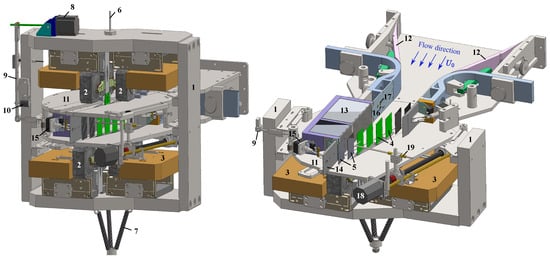
Figure 1.
Configuration of the test section. The blue arrows represent the flow direction. The components are designated as follows: 1—frame body; 2—electromagnetic shakers; 3—damper mass of electromagnetic shaker; 4—flexibly mounted blade (marked in green); 5—rigid blade (marked in gray); 6—steel rope; 7—frame spring; 8—frameshift stepper motor; 9—frame lever; 10—lever spring; 11—rotating disk; 12—adjustable inlet nozzle walls; 13—muffler; 14—directional flaps; 15—stepper motor of directional flap; 16—flush-mounted static port; 17—Pitot probe; 18—traversing system; 19—probe support.
Instrumentation consists of a flush-mounted static port, a Pitot probe, and a thermocouple upstream of the blade cascade to measure the inlet flow velocity. A traversing system with a probe holder is also positioned downstream for further measurements. The blades’ bending y and torsional a motions were determined using signals from two Schenck IN-085 eddy (Schenck, Deer Park, NY, USA) current displacement sensors.
2.2. Blade Cascade and Experimental Setup
As previously mentioned, the blade cascade consists of eight blades, four of which are movable. A schematic representation of the vibrating blade cascade is shown in Figure 2. The blades under investigation are made from metal and represent a scaled-down model of the tip profile of a steam turbine rotor’s last-stage blade. The blade geometry is defined by a chord length of , a span of , and a maximum thickness of . The incidence angle of the blades within the cascade is set at , with a pitch of and a cascade stagger angle of . The height and width of the inlet flow channel were and , respectively.
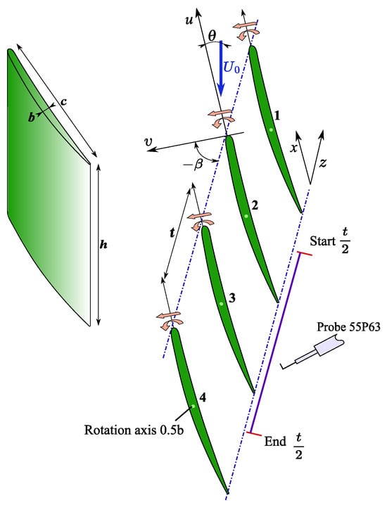
Figure 2.
Geometry of the turbine blade cascade end experimental setup. The blue arrow indicates the flow direction, while the blue line represents the hot-wire measurement cross-section. Here, and correspond to the cascade stagger angle and incidence angle of the blades, respectively.
The study investigated flow patterns under three distinct modes: stationary blade, bending vibrations, and torsional vibrations. Moreover, in the first scenario (ES.I), the study focused on the motion of an individual blade. In contrast, the second scenario (ES.II) examined the bending motion of the entire blade cascade with inter-blade phase angle variation. The experiments conducted at the flow velocity corresponding to a chord-based Reynolds number of , calculated based on the inlet flow velocity and the chord length of the blade, applying the relation (). The turbulence intensity of the inflow was less than 0.2%, and the excitation frequency of the vibrating blades was 72.8 Hz. The oscillation amplitudes for torsion and bending modes were and . Measurements were conducted at a cross-section 3 mm downstream of the trailing edge, at mid-blade height, corresponding to . The measurement region covered two pitch periods, including blades 2 and 3, with a step of 1 mm between measurement points.
The experimental study employed a constant temperature anemometer (hot-wire anemometer) with a miniature X-wire probe (Type 55P63). This configuration facilitated a detailed two-dimensional turbulent flow structure analysis, encompassing the streamwise u and spanwise v components, as described by [16,17]. The wire probes, coated with tungsten and platinum, feature a diameter of 5 μm and an active length of 1.25 mm, with gilded wire ends. Hot-wire signals in all experiments were sampled at a frequency of 250 kHz and signal filtering was applied. The high-pass and low-pass filter cut-off frequencies were set at 10 Hz and 60 kHz, respectively. Each single-point measurement lasted 10 s.
2.3. Calibration Principle of and Uncertainty Analysis
The fundamental principle of the constant temperature anemometer is to maintain the thermal state of the hot wire by compensating for heat loss [16,17]. When exposed to fluid flow, the anemometer’s wire loses heat to the surrounding medium, with convective heat transfer mainly determined by the fluid’s velocity. As a result, the wire’s temperature and electrical resistance vary. A Wheatstone bridge circuit measures these resistance changes in response to temperature fluctuations. The system continuously supplies additional energy to counteract the cooling of the wire, ensuring it remains at a constant temperature. Therefore, the power required for this stabilization is directly related to the fluid flow rate detected by the sensor.
The Collis-Williams law was applied for the calibration and estimation of instantaneous flow velocity [18,19]. In this framework, the behavior of the wire during cooling in the flow can be described by the Equation (1). The left part of the equation represents the heat transfer process, while the right one corresponds to the formulation of King’s law [20].
where the A, B, M, N are calibration constants. Notably, the values of A and B depend on the wire’s temperature and dimensions [21]. The Nusselt number and the wire Reynolds number can be calculated following the methodology outlined by Bruun [22]. Wheres, the effective temperature is defined by the following equation:
here T and represent the ambient and hot-wire temperatures, respectively, measured in Kelvin.
To determine the parameters in Equation (1), experimental measurements were performed within a test velocity range of 33 to 75 m · s−1. The collected data were applied to construct calibration curves of and (Figure 3), which were subsequently fitted to King’s law This process enabled the determination of the calibration constants A, B, M, and N. With their help, it is easy to find the wire Reynolds number, which corresponds to the characteristic Nusselt number obtained from the hot-wire signal: This process determined the calibration constants A, B, M, and N, facilitating the calculation of the wire Reynolds number corresponding to the characteristic Nusselt number from the hot-wire signal.
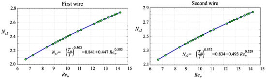
Figure 3.
Sample hot-wire blowdown calibration curve for first and second wire. Accordingly, the and are streamwise and span components. The blue line illustrates the calibration curve, while the green dots represent the experimental data.
Finally, the instantaneous velocity can be easily calculated using the following equation:
where and are wire diameter and kinematic viscosity of air, respectively.
As observed in Figure 3, the obtained calibration curves exhibit good agreement with the experimental data. The precision uncertainty in velocity measurements was estimated using classical methodologies [23,24]. Analysis of the obtained data reveals that the overall uncertainty in converting the hot-wire electrical signal to velocity is approximately . This value remains nearly identical for measurements in streamwise and spanwise directions.
3. Results and Discussion
3.1. Wake Topology
Initially, the vibrating effect on the wake topology downstream of the blade cascade was evaluated. Figure 4 compares of the normalized streamwise and spanwise velocity component distributions under different experimental scenarios. For better visualization, the measurement positions of the collected data were normalized by the pitch. Consequently, the trailing edges of blades 2 and 3 were located at and , respectively.
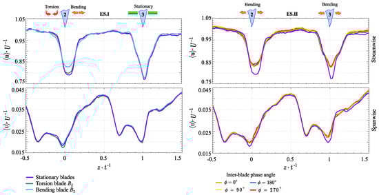
Figure 4.
Distribution of normalized streamwise and spanwise velocity components across experimental scenarios.
The findings demonstrate a strong effect of the bending mode on wake topology, resulting in a 5% reduction in the streamwise velocity deficit compared to the stationary and torsion modes. Additionally, obtained profiles of across both experimental scenarios show a consistent displacement of the wake center toward the suction side. This behavior is attributed to the expansion of the boundary layer on the suction side, driven by the blade’s asymmetric geometry and angle of attack [25]. Unexpectedly, the data also highlight deviations in the wake shapes behind different blades, which persist even under stationary conditions. Specifically, blade 3 exhibits a slightly higher velocity deficit and a broader wake in the streamwise direction compared to blade 2. These discrepancies are likely due to difficulties in achieving precise dynamic balance and positioning each blade within the cascade. However, the wake depth remains uniform across all blades under the bending motion of the entire blade cascade. Meanwhile, the spanwise velocity distribution remains largely unaffected across the different experimental scenarios.
The flow behavior around a vibrating blade is a complex phenomenon closely connected to turbulence [26]. Consequently, the analysis of turbulent kinetic energy (TKE) and turbulence intensity (TI) offers critical insights into understanding the impact of blade vibration on the wake topology. From a physical perspective, TKE quantifies the energy contained within the turbulent flow, while TI characterizes the level of its perturbation. For two-dimensional flow, they can be expressed by classical relation:
and
where and denote the time-averaged velocity fluctuations, while and represent the mean velocities in the streamwise and spanwise directions, respectively.
Figure 5 presents the normalized distribution of turbulent kinetic energy and turbulence intensity across various experimental scenarios. The results indicate a pronounced influence of the bending mode on the turbulent kinetic energy and intensity of turbulence in the wake region. In comparison to the stationary and torsional modes, the maximum value of TKE and TI increase 1.52 and 1.25 times, respectively. This effect is largely explained by the specific mechanism of vortex formation caused by the blade motion.
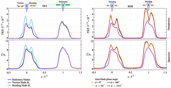
Figure 5.
Normalized turbulent kinetic energy and turbulence intensity distributions across experimental scenarios.
Flow separation occurs later in the stationary and torsional modes than in the bending mode. This process is followed by rolling up and recirculating the shear layer on the suction side. As a result, smaller vortex structures continuously form over time in stationary and torsional modes. In contrast, the bending mode alters this process, causing an earlier onset of flow separation and resulting in the formation of larger dynamic vortices [2,7]. These structures exhibit higher turbulent kinetic energy, contributing to increased flow instability compared to the stationary and torsion modes.
Furthermore, the comparative analysis highlighted differences in the shapes of the obtained distributions. Specifically, the stationary and torsion modes typically generate a single peak, whereas the bending mode leads to the formation of double peaks. The observed discrepancy is primarily attributed to the distinct characteristics of the vortex propagation mechanism. The formation of a single peak can be attributed to the amplification of vortices passing from the suction side by those from the pressure side [27]. This interaction leads to the formation of a dominant vortex within the overall flow. In contrast, a double peak indicates the simultaneous propagation of vortices from both sides of the blade.
Flatness, also known as kurtosis, is another crucial parameter for evaluating wake characteristics [28]. In turbulent flows, high flatness indicates strong bursts (or spikes) in velocity fluctuations, a key feature of intermittency [29]. Additionally, flatness provides important insights into the edge of the shear layer region, where large-scale coherent structures break down into smaller eddies. Mathematically, flatness can be expressed by the classical relation:
where is standard deviation of the streamwise velocity component.
Figure 6 shows a flatness distribution obtained across experimental scenarios. The results reveal that the highest flatness occurs during the bending mode, which is about 1.7 times greater than in the stationary mode. These observations indicate that blade vibration significantly increases flow instability. Notably, extreme values are consistently observed on both sides of the blade, appearing as distinct peaks.
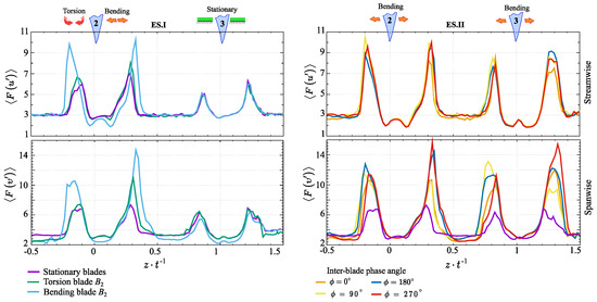
Figure 6.
Flatness distributions across experimental scenarios.
This regularity is consistently observed across all experimental modes and is equally evident in streamwise and spanwise directions. Furthermore, the analysis of the resulting distributions for various motion modes reveals that, in the case of bending, the distance from the trailing edge to the point of maximum flatness values increases. This pattern suggests a corresponding expansion of the shear layer width. The primary factor causing this phenomenon is the displacement of the separation point toward the leading edge. As a result, a shear layer forms earlier, characterized by higher levels of turbulence intensity.
A comparison of the collected data suggests that the bending motion leads to the formation of larger vortices, commonly referred to as “shear layer vortices”. These vortices are typically the most energetic structures within the flow. As they approach to the edge of the shear layer, they become unstable and eventually breakdown into the free stream. However, it should be noted that, the intensity of this process is strongly dependent on the blade’s motion. Figure 6 illustrates that, within the torsion mode, the maximum flatness values are predominantly concentrated on the suction side. This phenomenon is primarily attributed to the blade’s geometry and its angular motion around axis. Thus, a pronounced flow separation region develops on the suction side, accompanied by strong dynamic vortex disruptions. Whereas, on the pressure side, the bent configuration and angular oscillation of the blade contribute to the dissipation of flow energy.
3.2. Reynolds Stress Components
The complete description of the instantaneous state of an incompressible fluid field relies on a set of Navier-Stokes equations complemented by a continuity equation. However, implementing the solutions for these instantaneous states in practice applications is challenging due to various factors. Therefore, Reynolds suggested adjusting the mathematical model to estimate statistically averaged states. This interpretation was later named after him as the “Reynolds equations”:
where I is a part which represents stress caused by mean pressure, II is a stress tensor associated with mean viscosity, III is Reynolds stress tensor created through the fluctuation part of the flow.
The III term is usually called as “Reynolds stress tensor”, which is mathematically represented as a second-order symmetric semi-definite tensor (see Equation (9)). From a physical point of view, this tensor can be understood as the average transfer of momentum in the i direction due to fluctuating motion in the k direction, or conversely, the transfer of momentum in the k direction caused by fluctuations in the i direction. Thus the diagonal elements of are associated with normal stress , whereas non-diagonal elements , describe shear stress. Classically, the Reynolds stress tensor describes a three-dimensional flow (u, v, w), disregarding the density’s negative impact . However, in our case, a hot-wire anemometer with a 55P63 X-wire probe was applied for experiments, enabling the investigation of turbulent flow in the streamwise and spanwise directions. As a result, the Reynolds stress tensor was statistically two-dimensional.
Figure 7 presents the distributions of the normalized Reynolds stress components across the experimental scenarios. The obtained data reveals a pronounced impact of the blade modes on the streamwise Reynolds normal stress component. Namely, in the bending mode, the value of is nearly 3 times greater compared to the torsion and stationary modes. This pattern is primarily explained by the effective energy injection into the flow due to the active blade’s motion. Consequently, velocity fluctuations in the near-surface blade region are intensified, resulting in increased flow perturbations within the wake. However, this effect is absent in the torsion mode. It can be attributed to a higher vortex energy dissipation rate, which is potentially driven by the blade’s angular motion. In contrast, the spanwise direction demonstrates minimal variation in the value of across different experimental scenarios.
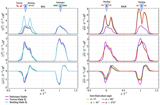
Figure 7.
Normalized distribution of Reynolds stress components across experimental scenarios.
The distribution of the Reynolds shear stress component is also shown in Figure 7. Physically, this component is associated with the diffusion mechanism for transport of fluid momentum. Graphically, it exhibits a characteristic asymmetric distribution, marked by a pattern of alternating positive and negative values along the wake centerline. The obtained distribution clearly delineates the region of flow instability, where the turbulence structure exhibits anisotropic characteristics. Namely, when the flow fluctuations are statistically uniform in all directions, the shear stresses goes to zero and the normal stresses become equal. Otherwise at and the turbulent flow is anisotropic [30,31,32]. It can be observed that the perturbation area with negative values is located directly on the pressure side. Usually, negative values are attributed to the progress of turbulent intensity, which increases frictional resistance in the average flow. As a result, energy is transferred to the turbulence, leading to a corresponding loss in the average flow.
The distributions shown in Figure 7 demonstrate that the bending mode exhibits the minimum values of , while the torsion and stationary modes are associated with the maximum values. These results are somewhat unexpected since although the Reynolds shear stress is higher in the last cases, the turbulent kinetic energy and turbulence intensity remain lower compared to the bending mode (see Figure 5). This is primarily due to the different mechanisms of turbulence generation associated with blade movement. Namely, in the bending mode, uniform blade vibrations generate large-scale coherent structures and an expanded shear layer, leading to elevated turbulence intensity and turbulent kinetic energy. However, energy dissipation is less provided, as the energy is distributed across larger-scale vortices. These vortices dominate in the flow, but their broad distribution results in weaker velocity gradients and reduced Reynolds shear stress component. In contrast, the blade’s angular motion in the torsion mode creates stronger velocity gradients, which improve turbulent momentum transport, thereby increasing the Reynolds shear stress component. The turbulence in this mode is characterized by small-scale structures, which lead to higher energy dissipation rates. Meanwhile, obtained data reveals that variations in the interblade phase angle during the bending mode have a minimal impact on the formation of Reynolds stress components.
3.3. The Spectral Analysis
Turbulent flows have a complex structure characterized by different spatial scales. Power spectral density (PSD) is widely employed to analyze the distribution of energy flux intensity across these scales. The Welch method, widely used for PSD estimation, improves accuracy by segmenting signals and averaging to reduce noise. This makes it practical for analyzing noisy signals with broad dynamic ranges.
Measurement points A and B were selected for the spectral analysis of turbulent flow around blade two under various experimental conditions. These points correspond to areas of maximum turbulent kinetic energy in the wake, specifically for the streamwise component (as depicted in Figure 5). The main difference between these two points lies in their locations: point A is on the pressure side, whereas point B is on the suction side.
Figure 8 illustrates the Welch power spectral densities of streamwise velocity fluctuations at measurement points A and B across different experimental scenarios. The obtained spectra exhibit a dynamic range spanning eight orders of magnitude (from 100 at low frequency to at high frequency before noise occurs at frequencies above ). The obtained distributions exhibit localized power bursts marked by distinct peaks. From a turbulence perspective, pronounced spikes in signal power typically indicate the presence of large-scale vortex structures. However, the mechanisms driving the formation of these structures differ.
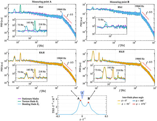
Figure 8.
Welch power spectral density distribution across experimental scenarios.
The peaks below 300 Hz are primarily associated with the blade’s vibratory motion, indicating active vortex breakdown propagation in the wake region. Specifically, the peaks at 73, 145, and 218 Hz correspond to the blade’s excitation frequency’s first, second, and third harmonics. In contrast, the spectral peak at 19,860 Hz is attributed to the vortex shedding frequency.
Under the first scenario, all three harmonics are distinctly identified on the pressure side at point A, while only the first harmonic is evident on the suction side at point B. This distribution underscores the substantial influence of the blade’s motion on the formation of large-scale vortex structures, particularly on the pressure side, where the highest power peaks are associated with the bending mode. In contrast, under the second scenario, the spectral distributions reveal that the simultaneous vibration of all cascade blades significantly enhances vortex generation on the suction side. Unlike the first scenario, all three harmonics are present in this case.
Furthermore, the spectral distributions measured at points A and B exhibit a curve segment in the 20 to 50 kHz frequency range, with a slope of . According to [33], this segment corresponds to the inertial range, where kinetic energy transfer across turbulence scales is governed solely by the energy dissipation rate. Moreover, this feature reflects the presence of statistically uniform turbulent fluctuations in streamwise and spanwise transverse directions.
4. Turbulence Structure Evaluation
From a physical standpoint, turbulence consists of discrete disturbances interacting and propagating within the flow. Hot-wire turbulence measurements are usually performed at fixed spatial points, producing time-series data from sequences of numerous disturbances or vortices. The dynamics of sufficiently separated vortices in space or time tend to exhibit statistical independence [34,35]. Therefore, the measured signal is treated as a random process and analyzed using statistical methods. This approach enables the determination of time-averaged properties of the entire vortex array.
In a turbulent flow, energy transfer is primarily provided by the most energetically dominant vortices, the average size of which is determined by the integral scale. Conversely, the smallest eddies play a crucial role in the process of energy dissipation and are associated with the Taylor and dissipation or Kolmogorov microscales [36,37,38]. It is essential to highlight that, despite their proximity, the Taylor and Kolmogorov microscales are fundamentally different. The Taylor microscale indicates the length scale at which energy dissipation starts to outweigh energy transfer, effectively marking the end of the integral scale. In contrast, the Kolmogorov microscale defines the dimensions of the smallest eddies, where significant energy dissipation occurs. Evaluating the integral scale can be accomplished using various methods based on different statistical approaches. These methods can be broadly categorized into two groups: those that utilize correlation analysis and those that rely on spectral density estimation.
This section presents the analysis of the turbulence structure under different blade motion modes, focusing on the dominant streamwise u-component of the flow.
4.1. Integral Length Scale
The initial step in analyzing turbulence structures typically involves determining the integral length scale. One commonly used method for estimating this scale is the correlation method [39]. Mathematically, the autocorrelation function measures the degree of correlation between velocity fluctuations as a function of the spatial gap between two data samples.
where represents the ensemble average, and is the spatial scale determined by Taylor’s classical “frozen turbulence” hypothesis. This approach converts a temporal increment from the recorded signal into a spatial increment, given . Meanwhile, denotes the variance of the streamwise velocity fluctuations.
The behavior of the autocorrelation function provides valuable insights into turbulent structures [40,41]. A smooth correlation curve indicates the presence of uniform vortices, while a distorted curve suggests multiple coexisting vortices. Most importantly, the point at which the autocorrelation function intersects the spatial axis corresponds to the size of the largest eddies. The autocorrelation function typically ranges between . However, in some cases, it stabilizes at a non-zero threshold. This phenomenon is particularly prominent in turbulent flows, where persistent large-scale vortices maintain non-zero mean values. Turbulent flow features a variety of large-scale structures, making cumulative integration a standard method for determining their average size .
where is the autocorrelation function of the streamwise component u in spatial domain .
The threshold value selection notably affects the integration region when calculating the integral length scale. While Kolmogorov et al. traditionally propose a zero threshold for the correlation coefficient, alternative values, such as 0.2 or , are also commonly used [42,43,44].
In addition to the correlation method for evaluating turbulent flow structures, the approaches proposed by Roach and von Kármán are also widely applied in engineering practice. While both methods rely on spectral flow analysis, they are grounded in fundamentally different physical principles. In Roach’s approach, the integral length scale is determined from the energy spectrum distribution of turbulent structures [45].
where denotes the average value calculated from the first 500 data points within the energy spectrum distribution .
In contrast, von Kármán proposed an alternative method for estimating the integral length scale based on identifying the maximum frequency corresponding to the dominant vortices [46].
where maximum frequency of the normalized power spectrum distribution .
Figure 9a,b present a comparative analysis of the integral length scale obtained through different methods for the stationary and bending modes of the blade, respectively. The distributions show strong agreement in the stationary mode, with the maximum integral length scale reaching 23 mm. However, significant differences emerge between the estimation methods in the bending mode, particularly in the wake region. Specifically, the correlation and von Kármán methods indicate integral length scales of approximately mm and mm, respectively. These values notably exceed the inter-blade spacing, which is only 23 mm. In contrast, the Roach approach suggests that the maximum vortex size is limited to the inter-blade space.
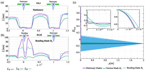
Figure 9.
(a,b) provides a comparative assessment of the integral length scale determined by different approaches for the stationary and bending modes, respectively. Here, corresponds to the autocorrelation approach, to the Roach method, and to the von Kármán method. (c) Autocorrelation function of streamwise velocity fluctuation at the measurement point N depending on the blade motion mode.
The discrepancy observed in the correlation method largely stems from the challenge of determining the threshold value, particularly during blade vibrations. This issue arises because the autocorrelation function exhibits periodic behavior, as illustrated in Figure 9c. In contrast, the von Kármán method is affected by the blade’s vibratory motion, which generates spikes in the spectral distribution, leading to significant estimation distortion. Therefore, Roach’s method was chosen for further evaluation of the integral length scale.
Figure 10 shows the distribution of the integral length scale across different experimental scenarios. The data indicate fivefold increases in the size of the largest vortices in the bending mode and twofold in the torsion mode compared to the stationary mode. This feature is due to the distinct characteristics of vortex formation under various blade modes. Additionally, variations in the inter-blade phase angle do not significantly affect the integral length scale.
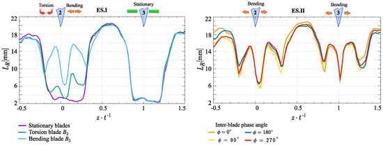
Figure 10.
Integral length scale distributions across various experimental scenarios.
4.2. Energy Dissipation Rate
The energy dissipation rate is a fundamental quantity that characterizes the rate at which turbulent kinetic energy dissipates into heat due to viscosity [47]. This rate can derive from various statistical quantities, ranging from the dissipative and inertial range to the energy injection sub-range [48].
In equilibrium turbulence, the rate of kinetic energy transfer across eddies of a particular size remains constant within the inertial range, assuming the Reynolds number is sufficiently high [49]. This transfer rate can be described through dimensional analysis as , where is the characteristic velocity scale of eddies with length L. By considering the integral scale L and its corresponding velocity scale , defined as the root-mean-square velocity fluctuation , the mean energy dissipation rate in the energy injection range can be calculated, as outlined by Taylor [50].
where denotes the dissipation constant, which ranges from 0.5 to 0.73 [51,52,53].
Kolmogorov’s second similarity hypothesis, proposed in 1941, offers an alternative approach for estimating the energy dissipation rate within the inertial range [54]. This method utilizes the scaling behavior of the second-order longitudinal structure function in the inertial range, allowing the calculation of the mean energy dissipation rate [32].
where C is a empirical constant [32], while is longitudinal second-order structure function.
In experiments, direct measurement of is often not feasible. Assuming statistically homogeneous and isotropic turbulence, the volume- and time-averaged energy dissipation rate in the dissipative sub-range can be estimated using a longitudinal velocity gradient [50,55,56,57,58].
where represents the kinematic viscosity, is the mean velocity, denotes spatial derivative of the velocity component , and indicates time averaging.
Moreover, suppose the spatial increment is smaller than the Kolmogorov microscale . The in the dissipative sub-range can also be determined using a longitudinal second-order structural function [59,60].
Figure 11 presents a comparative analysis of the energy dissipation rate calculated by various approaches for the stationary and bending modes. The results demonstrate a strong agreement between different methodologies, particularly in the bending mode. For further analysis, the energy dissipation rate, denoted as , was evaluated within the inertial subrange. As shown in Figure 12, the maximum value of 4200 occurs in the stationary mode, while the minimum value of 3400 is observed in the bending mode. Notably, the highest values consistently appear on the pressure side. Additionally, the obtained distributions reveal that the inter-blade phase angle does not affect the energy dissipation rate in the bending mode.
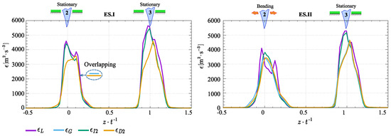
Figure 11.
Comparison of the energy dissipation rate calculated by different approaches. Here is the method based on a scaling argument (energy injection range), is the method based on second-order structure function (inertial sub-range), is the method based on longitudinal velocity gradient (dissipation sub-range), is the method based on second-order structure function (dissipative sub-range).
Figure 12.
Energy dissipation rate distributions across various experimental scenarios.
4.3. Kolmogorov and Taylor Microscale
Once the dissipation rate is known, Taylor and Kolmogorov microscales can be estimated from classical relations:
and
Figure 13 shows the Taylor microscale growth in the wake region under bending mode. Specifically, the value of nearly doubles when compared to the stationary and torsion modes. Additionally, variations in the inter-blade phase angle under collective blade motion further increase the value of . Notably, within the inter-blade space at , the Taylor microscale grows to 3 mm, whereas at other values, it remains around 2 mm.
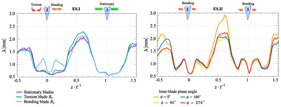
Figure 13.
Taylor microscale distributions across various experimental scenarios.
Unlike the Taylor microscale, the Kolmogorov microscale distributions remain nearly unchanged across different blade motion modes. As shown in Figure 14, the smallest eddies of are observed in the wake region, while in the inter-blade region, their size increases up to . As noted earlier, the Kolmogorov microscale characterizes the size of the eddies responsible for energy dissipation. This relationship is evident in the comparative analysis of Figure 12 and Figure 14, where a decrease in corresponds to an increase in .
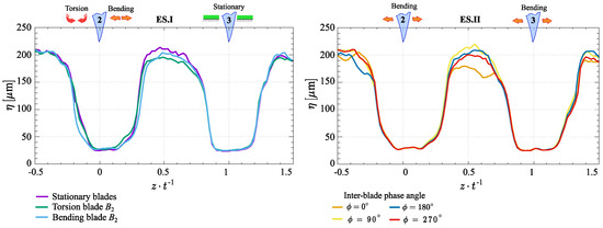
Figure 14.
Kolmogorov microscale distributions across various experimental scenarios.
Finally, the Reynolds number based on Taylor microscales , was calculated using Equation (21).
The data shown in Figure 15 illustrate the significant effect of bending motion on the Reynolds number based on Taylor microscales. Specifically, shows a sharp increase in the wake region, rising nearly 2.5 times compared to the stationary and torsion modes. This phenomenon arises from enhanced energy transfer from larger to smaller structures and intensified vortex formation driven by blade vibrations.
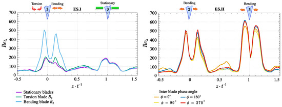
Figure 15.
Distributions of the Reynolds number based on the Taylor microscale across experimental scenarios.
5. Conclusions
The study investigated the impact of blade vibrations on the wake topology and turbulence structure downstream of a low-pressure turbine blade cascade. The experiments used hot-wire anemometry with an X-wire probe at a flow velocity corresponding to a chord-based Reynolds number of , where mm. A comparative analysis of flow patterns between a stationary blade and those during its bending and torsion vibrations was conducted. The excitation frequency of the vibration was , with oscillation amplitudes of for torsion and 0.7 mm for bending mode.
The findings demonstrate a significant effect of the bending mode on wake topology, leading to a 5% reduction in the streamwise velocity deficit compared to the stationary and torsion modes. Additionally, in the wake region, the bending mode increases turbulent kinetic energy and turbulence intensity 1.52 and 1.25 times, respectively. This effect is primarily attributed to the vortex generation mechanism caused by blade motion. Specifically, the bending mode causes an earlier onset of flow separation, expanding the shear layer where large-scale coherent structures actively form. These structures, commonly referred to as “shear layer vortices”, exhibit high turbulent kinetic energy and contribute to enhanced flow instability. Notably, flatness analyses across various blade modes confirm the greatest expansion of the shear layer and heightened vortex breakdown activity in the bending mode.
The Reynolds stress components were also employed to assess the flow pattern around the vibrating blade. The obtained data indicate a 1.25 times increase of the streamwise Reynolds normal stress component in the bending mode compared to the stationary and torsion modes. This phenomenon is primarily attributed to the efficient energy injection into the flow. As a result, velocity fluctuations in the near-surface blade region intensify, causing enhanced flow perturbations in the wake. In contrast, this effect does not occur in the torsion mode, likely due to the increased energy dissipation rate associated with the blade’s angular motion.
The power spectral density method evaluated the distribution of energy flux intensity across different spatial scales in turbulent flow. The findings emphasize the significant role of the bending mode in generating large-scale vortices. Vortex formation is more pronounced on the pressure side in the case of single-blade oscillation. However, the synchronized oscillation of all cascade blades significantly enhances vortex formation on the suction side.
Finally, the turbulence structure was estimated under different experimental conditions. The integral length scale, determined using the Roach method, shows that the size of the largest vortices increases fivefold in the bending mode and 2 times in the torsion mode compared to the stationary configuration. Additionally, in the bending mode, the Taylor microscale in the wake region increases twofold, while the Kolmogorov microscale distribution remains unchanged mainly across various scenarios. Furthermore, the findings indicate that bending vibrations reduce the energy dissipation rate by 20% and increase the Taylor-microscale Reynolds number 2.5 times relative to the stationary mode.
Author Contributions
Conceptualization, methodology, V.U., V.Y. and H.K.; validation, V.Y., D.D. and V.T.; formal analysis, V.Y. and H.K.; investigation, V.Y. and V.T.; writing—original draft preparation, writing—review and editing, V.Y. and V.U.; visualization, V.Y., D.D. and H.K.; supervision, V.U. All authors have read and agreed to the published version of the manuscript.
Funding
This research is supported by project “Investigation of 3D flow structures and their effects on aeroelastic stability of turbine-blade cascades using experiment and deep learning approach" GACR 24-12144S of the Grant Agency of the Czech Republic.
Data Availability Statement
Data are contained within the article.
Acknowledgments
This research is supported by project “Investigation of 3D flow structures and their effects on aeroelastic stability of turbine-blade cascades using experiment and deep learning approach” GACR 24-12144S of the Grant Agency of the Czech Republic.
Conflicts of Interest
The authors declare no conflict of interest.
References
- Srinivasan, A.V. Flutter and Resonant Vibration Characteristics of Engine Blades: An IGTI Scholar Paper. In International Gas Turbine and Aeroengine Congress and Exhibition; American Society of Mechanical Engineers: New York, NY, USA, 1997; p. No 97-GT-533. [Google Scholar] [CrossRef]
- Fürst, J.; Lasota, M.; Lepicovsky, J.; Musil, J.; Pech, J.; Šidlof, P.; Šimurda, D. Effects of a Single Blade Incidence Angle Offset on Adjacent Blades in a Linear Cascade. Processes 2021, 9, 1974. [Google Scholar] [CrossRef]
- Rahmati, M.; He, L.; Wells, R. Interface Treatment for Harmonic Solution in Multi-Row Aeromechanic Analysis. In Turbo Expo: Power for Land, Sea, and Air; American Society of Mechanical Engineers: Glasgow, UK, 2010; Volume 6, pp. 1253–1261. [Google Scholar] [CrossRef]
- Tucker, P. Computation of unsteady turbomachinery flows: Part 1—Progress and challenges. Prog. Aerosp. Sci. 2011, 47, 522–545. [Google Scholar] [CrossRef]
- Rahmati, M.; He, L.; Wang, D.; Li, Y.; Wells, R.; Krishnababu, S. Non-Linear Time and Frequency Domain Methods for Multi-Row Aeromechanical Analysis. In Turbo Expo: Power for Land, Sea, and Air; American Society of Mechanical Engineers: Copenhagen, Denmark, 2012; Volume 7, pp. 1473–1485. [Google Scholar] [CrossRef]
- Yang, H.; He, L. Experimental Study on Linear Compressor Cascade with Three-Dimensional Blade Oscillation. J. Propuls. Power 2004, 20, 180–188. [Google Scholar] [CrossRef]
- Nakhchi, M.; Rahmati, M. Direct numerical simulations of flutter instabilities over a vibrating turbine blade cascade. J. Fluids Struct. 2021, 104, 103324. [Google Scholar] [CrossRef]
- Peters, C.D.; van der Spuy, S.J.; Els, D.N.; Kuhnert, J. Aerodynamic damping of an oscillating fan blade: Mesh-based and meshless fluid structure interaction analysis. J. Fluids Struct. 2018, 82, 173–197. [Google Scholar] [CrossRef]
- Camp, T.R.; Shin, H.W. Turbulence Intensity and Length Scale Measurements in Multistage Compressors. J. Turbomach. 1995, 117, 38–46. [Google Scholar] [CrossRef]
- Oro, J.; Argüelles Díaz, K.; Santolaria, C.; Marigorta, E. On the structure of turbulence in a low-speed axial fan with inlet guide vanes. Exp. Therm. Fluid Sci. 2007, 32, 316–331. [Google Scholar] [CrossRef]
- Maunus, J.; Grace, S.; Sondak, D.; Yakhot, V. Characteristics of Turbulence in a Turbofan Stage. J. Turbomach. 2012, 135, 021024. [Google Scholar] [CrossRef]
- Odier, N.; Duchaine, F.; Gicquel, L.; Staffelbach, G.; Thacker, A.; García Rosa, N.; Dufour, G.; Muller, J.D. Evaluation of Integral Turbulence Scale Through the Fan Stage of a Turbofan Using Hot Wire Anemometry and Large Eddy Simulation. In Turbo Expo: Turbomachinery Technical Conference and Exposition; American Society of Mechanical Engineers: Oslo, Norway, 2018; Volume 2C, p. V02CT42A021. [Google Scholar] [CrossRef]
- Bauinger, S.; Behre, S.; Lengani, D.; Guendogdu, Y.; Heitmeir, F.; Göttlich, E. On Turbulence Measurements and Analyses in a Two-Stage Two-Spool Turbine Rig. J. Turbomach. 2016, 139, 071008. [Google Scholar] [CrossRef]
- Schwarzbach, F.; Müller-Schindewolffs, C.; Bode, C.; Herbst, F. The Effect of Turbulent Scales on Low-Pressure Turbine Aerodynamics: Part B—Scale Resolving Simulations. In Turbo Expo:Turbomachinery Technical Conference and Exposition; American Society of Mechanical Engineers: Oslo, Norway, 2018; Volume 2B, p. No V02BT41A005. [Google Scholar] [CrossRef]
- Eret, P.; Tsymbalyuk, V. Experimental Subsonic Flutter of a Linear Turbine Blade Cascade with Various Mode Shapes and Chordwise Torsion Axis Locations. J. Turbomach. 2022, 145, 061002. [Google Scholar] [CrossRef]
- Bruun, H. Interpretation of a hot wire signal using a universal calibration law. Phys. Sci. Instrum. 1971, 4, 225–231. [Google Scholar] [CrossRef]
- Bruun, H. Hot wire data corrections in low and in high turbulence intensity flows. J. Phys. Sci. Instrum. 1972, 5, 812–818. [Google Scholar] [CrossRef]
- Jonás, P. Rotary slanted single wire CTA—A useful tool for 3D flows investigations. EPJ Web Conf. 2013, 45, 01047. [Google Scholar] [CrossRef]
- Nix, A.; Smith, A.; Diller, T.; Ng, W.; Thole, K. High Intensity, Large Length-Scale Freestream Turbulence Generation in a Transonic Turbine Cascade. In Turbo Expo:Power for Land, Sea, and Air; American Society of Mechanical Engineers: Amsterdam, The Netherlands, 2002; Volume 3, pp. 961–968. [Google Scholar] [CrossRef]
- King, L.V.; Barnes, H.T. On the convection of heat from small cylinders in a stream of fluid: Determination of the convection constants of small platinum wires, with applications to hot-wire anemometry. Proc. R. Soc. Lond. Ser. A Contain. Pap. Math. Phys. Character 1914, 90, 563–570. [Google Scholar] [CrossRef]
- Andrews, G.E.; Bradley, D.; Hundy, G. Hot wire anemometer calibration for measurements of small gas velocities. Int. J. Heat Mass Transf. 1972, 15, 1765–1786. [Google Scholar] [CrossRef]
- Bruun, H.H. Hot-Wire Anemometry: Principles and Signal Analysis; Oxford University Press: Oxford, UK, 1995; p. 507. [Google Scholar] [CrossRef]
- Finn, E. How to Measure Turbulence with Hot-Wire Anemometers—A Practical Guide; Dantec Dynamics A/S: Skovlunde, Denmark, 2002; p. 54. [Google Scholar]
- Standard PTC 19.1-2018 (R2024); Test Uncertainty. American Society of Mechanical Engineers: New York, NY, USA, 2019.
- Duda, D.; Yanovych, V.; Tsymbalyuk, V.; Uruba, V. Effect of Manufacturing Inaccuracies on the Wake Past Asymmetric Airfoil by PIV. Energies 2022, 15, 1227. [Google Scholar] [CrossRef]
- Velarde-Suarez, S.; Ballesteros-Tajadura, R.; Santolaria, C.; Blanco-Marigorta, E. Total Unsteadiness Downstream of an Axial Flow Fan With Variable Pitch Blades. J. Fluids-Eng.-Trans. Asme—J. Fluids Eng. 2002, 124, 280–283. [Google Scholar] [CrossRef]
- Yanovych, V.; Duda, D.; Uruba, V.; Antoš, P. Anisotropy of turbulent flow behind an asymmetric airfoil. SN Appl. Sci. 2021, 3, 1–16. [Google Scholar] [CrossRef]
- Daniel, D.; Vaclav, U.; Yanovych, V. Wake Width: Discussion of Several Methods How to Estimate It by Using Measured Experimental Data. Energies 2021, 14, 4712. [Google Scholar] [CrossRef]
- Veerasamy, D.; Atkin, C. A rational method for determining intermittency in the transitional boundary layer. Exp. Fluids 2020, 61, 11. [Google Scholar] [CrossRef]
- Lumley, J.L.; Newman, G.R. The Return to Isotropy of Homogeneous Turbulence. J. Fluid Mech. 1977, 82, 161–178. [Google Scholar] [CrossRef]
- Choi, K.S.; Lumley, J. The return to isotropy of homogeneous turbulence. J. Fluid Mech. 2001, 436, 59–84. [Google Scholar] [CrossRef]
- Pope, S.B. Turbulent Flows, 1st ed.; Cambridge University Press: Cambridge, UK, 2000. [Google Scholar] [CrossRef]
- Kolmogorov, A. Dissipation of Energy in Locally Isotropic Turbulence. Proc. R. Soc. Lond. Ser. A Math. Phys. Sci. 1991, 1890, 15–17. [Google Scholar] [CrossRef]
- Davies, P. Structure of turbulence. J. Sound Vib. 1973, 28, 513–526. [Google Scholar] [CrossRef]
- Tropea, C.; Yarin, A.; Foss, J.F. Springer Handbook of Experimental Fluid Mechanics; Springer: Heidelberg, Germany, 2007; p. 1557. [Google Scholar]
- Pouransari, Z.; Vervisch, L.; Johansson, A. Reynolds Number Effects on Statistics and Structure of an Isothermal Reacting Turbulent Wall-Jet. Flow Turbul. Combust. 2014, 92, 931–945. [Google Scholar] [CrossRef]
- Tennekes, H.; Lumley, J. A First Course in Turbulence, 1st ed.; The MIT Press: Cambridge, MA, USA, 1972; p. 300. [Google Scholar]
- Corrsin, S. The Structure of Turbulent Shear Flow (A. A. Townsend). SIAM Rev. 1979, 21, 581–583. [Google Scholar] [CrossRef]
- Bourgoin, M.; Baudet, C.; Kharche, S.; Mordant, N.; Vandenberghe, T.; Sumbekova, S.; Stelzenmuller, N.; Aliseda, A.; Gibert, M.; Roche, P.E.; et al. Investigation of the small-scale statistics of turbulence in the Modane S1MA wind tunnel. CEAS Aeronaut. J. 2018, 9, 269–281. [Google Scholar] [CrossRef]
- Yanovych, V.; Duda, D.; Uruba, V. Structure turbulent flow behind a square cylinder with an angle of incidence. Eur. J. Mech.—B/Fluids 2021, 85, 110–123. [Google Scholar] [CrossRef]
- Batchelor, G.K. The Theory of Homogeneous Turbulence; Cambridge University Press: New York, NY, USA, 1982; p. 197. [Google Scholar]
- Katul, G.G.; Parlange, M.B. Analysis of Land Surface Heat Fluxes Using the Orthonormal Wavelet Approach. Water Resour. Res. 1995, 31, 2743–2749. [Google Scholar] [CrossRef]
- Hinze, J. Turbulence: McGraw-Hill Series in Mechanical Engineering; McGraw-Hill: New York, NY, USA, 1975; p. 790. [Google Scholar]
- Tritton, D. Physical Fluid Dynamics, 2nd ed.; Clarendon Press: Oxford, UK, 1988; p. 536. [Google Scholar]
- Roach, P. The generation of nearly isotropic turbulence by means of grids. Int. J. Heat Fluid Flow 1987, 8, 82–92. [Google Scholar] [CrossRef]
- Trush, A.; Pospisil, S.; Kozmar, H. Comparison of Turbulence Integral Length Scale Determination Methods. Adv. Fluid Mech. XIII 2020, 11, 113–123. [Google Scholar] [CrossRef]
- Wang, G.; Yang, F.; Wu, K.; Ma, Y.; Peng, C.; Liu, T.; Wang, L.P. Estimation of the dissipation rate of turbulent kinetic energy: A review. Chem. Eng. Sci. 2021, 229, 116133. [Google Scholar] [CrossRef]
- Schröder, M.; Bätge, T.; Bodenschatz, E.; Wilczek, M.; Bagheri, G. Estimating the turbulent kinetic energy dissipation rate from one-dimensional velocity measurements in time. Atmos. Meas. Tech. 2024, 17, 627–657. [Google Scholar] [CrossRef]
- Lumley, J. Some comments on turbulence. Phys. Fluids A Fluid Dyn. 1992, 4, 203–211. [Google Scholar] [CrossRef]
- Taylor, G. Statistical theory of turbulence. Proc. R. Soc. Lond. Ser. A Math. Phys. Sci. 1935, 151, 421–444. [Google Scholar] [CrossRef]
- Sreenivasan, K. On the universality of the Kolmogorov constant. Phys. Fluids 1995, 7, 2778–2784. [Google Scholar] [CrossRef]
- Sreenivasan, K. An update on the energy dissipation rate in isotropic turbulence. Phys. Fluids 1998, 10, 528–529. [Google Scholar] [CrossRef]
- Pearson, B.; Krogstad, P.Å.; Van De Water, W. Measurements of the turbulent energy dissipation rate. Phys. Fluids 2002, 14, 1288–1290. [Google Scholar] [CrossRef]
- Kolmogorov, A. The local structure of turbulence in incompressible viscous fluid for very large Reynolds numbers. Dokl. Akad. Nauk. SSSR 1941, 30, 301–305. [Google Scholar] [CrossRef]
- Davidson, P. Turbulence: An Introduction for Scientists and Engineers, 2nd ed.; Oxford University Press: Oxford, UK, 2015. [Google Scholar] [CrossRef]
- Elsner, J.; Elsner, W. On the measurement of turbulence energy dissipation. Meas. Sci. Technol. 1996, 7, 1334. [Google Scholar] [CrossRef]
- Almalkie, S.; de Bruyn Kops, S. Energy dissipation rate surrogates in incompressible Navier–Stokes turbulence. J. Fluid Mech. 2012, 697, 204–236. [Google Scholar] [CrossRef]
- Champagne, F. The fine-scale structure of the turbulent velocity field. J. Fluid Mech. 1978, 86, 67–108. [Google Scholar] [CrossRef]
- Siebert, H.; Lehmann, K.; Wendisch, M. Observations of small-scale turbulence and energy dissipation rates in the cloudy boundary layer. J. Atmos. Sci. 2006, 63, 1451–1466. [Google Scholar] [CrossRef]
- Muschinski, A.; Frehlich, R.; Balsley, B. Small-scale and large-scale intermittency in the nocturnal boundary layer and the residual layer. J. Fluid Mech. 2004, 515, 319–351. [Google Scholar] [CrossRef]
Disclaimer/Publisher’s Note: The statements, opinions and data contained in all publications are solely those of the individual author(s) and contributor(s) and not of MDPI and/or the editor(s). MDPI and/or the editor(s) disclaim responsibility for any injury to people or property resulting from any ideas, methods, instructions or products referred to in the content. |
© 2025 by the authors. Licensee MDPI, Basel, Switzerland. This article is an open access article distributed under the terms and conditions of the Creative Commons Attribution (CC BY) license (https://creativecommons.org/licenses/by/4.0/).