Improved Vehicle Object Detection Algorithm Based on Swin-YOLOv5s

Abstract

In response to the challenges of low detection accuracy, slow speed, and high rates of false positives and missed detections in existing YOLOv5s vehicle detection models under complex traffic scenarios, an improved Swin-YOLOv5s vehicle detection algorithm is proposed in this paper. By incorporating the Swin Transformer attention mechanism to replace the original C3-1 network, the computational load is reduced and the capability of capturing global features is enhanced. The Self-Concat feature fusion method is enhanced to enable adaptive adjustment of the feature map weights, thereby enhancing positive features. The results of experiments conducted on the KITTI dataset and tests with the Tesla V100 indicate that the proposed improved Swin-YOLOv5s algorithm achieves a mean average precision (mAP) of 95.7% and an F1 score of 93.01%. These metrics represent improvements of 1.6% and 0.56%, respectively, compared to YOLOv5s. Additionally, the inference speed for a single image increases by 1.11%, while the overall detection speed in frames per second (FPS) improves by 12.5%. This enhancement effectively addresses issues related to false positives and missed detections encountered by YOLOv5s under severe vehicle occlusion conditions. The ablation experiments and comparative experiments with different network models validate both the efficiency and accuracy of this model, demonstrating its enhanced capability to meet practical vehicle detection requirements more effectively.

1. Introduction

The detection of vehicle targets is not only a critical task in intelligent transportation systems and autonomous driving but also serves as the foundation for the future development of traffic intelligence and automation. In recent years, this area has garnered increasing attention from numerous researchers. However, in practical applications, object detection continues to face numerous technical challenges. Firstly, the complex and variable traffic environment, along with the diverse sizes, shapes, and occlusion conditions of target objects, presents significant difficulties for object detection. Secondly, during driving scenarios, certain small vehicles occupy only a minimal portion of the image; this limitation results in very restricted feature information and increases the difficulty of detection [1,2]. To address these issues effectively, it is essential to improve detection algorithms based on real-world conditions in order to enhance the accuracy and recognition capability of vehicle detection models.

The current object detection algorithms can be categorized into two main types. The first type comprises traditional algorithms that identify objects by extracting their prominent features from images [3,4,5,6]. Examples include Haar [7] and HOG [8], which rely on manually extracted information such as color and shape to recognize vehicles. These methods are time-consuming, labor-intensive, and have significant limitations, making them ill suited for the advancements in autonomous driving technology. The second type involves deep learning algorithms that learn object features progressively through multiple layers. Scholars both domestically and internationally have begun extensive research due to its strong self-learning capabilities, high accuracy, and excellent real-time performance. In an international study, Tang et al. proposed a two-dimensional message-passing state estimation algorithm, establishing an “estimation-friendly” remote state estimation framework that effectively reduces computational complexity [9]. Geetha A S investigated five variants of YOLOv5—namely, YOLOv5n6s, YOLOv5s6s, YOLOv5m6s, YOLOv5i6s, and YOLOv5x6s—for vehicle detection across various environments. The findings suggested that the YOLOv5i6s variant was particularly suitable for car detection, while YOLOv5x6s demonstrated superior performance in recognizing buses and sedans [10]. Bakirci M conducted a detection study on drone flights based on the YOLOv8 model, achieving an accuracy rate of 80% [11]. The YOLOv5 model was also implemented on Raspberry Pi 4 to achieve real-time processing of aerial images captured by drones, resulting in an accuracy improvement of 88% [12]. The improved YOLOv5s algorithm, based on the multi-scale channel attention CBAM module, was employed to identify remote vehicle and pedestrian information. This enhancement accelerated the model’s convergence speed, achieving an average accuracy of 84.9% [13]. The GSConv and Slim Neck structures have been employed to replace the Neck structure of YOLOv5, thereby reducing the parameter count and computational complexity of the vehicle detection model [14]. In the domestic context, inspired by the Ghost module, a tunnel vehicle detection model based on GCM-YOLOv5s by replacing the original convolutional layers with the GhostConv module was proposed. This approach addressed, to some extent, the challenges of detecting and distinguishing vehicle types and traffic flow in complex traffic environments [15]. In response to the current challenges posed by the complexity of vehicle recognition neural network algorithms and their large number of parameters, the bneck module of MobileNetV3 was employed by Dengchao to replace the backbone network of YOLOv5s. Testing on the UA-DETRAC dataset revealed that this modification resulted in an 82.6% reduction in algorithm parameters compared to YOLOv5s [16]. An improved nighttime vehicle detection algorithm based on YOLOv5s and double-stable stochastic resonance was proposed. The experimental results indicated that this method demonstrated a high accuracy rate and a low missed detection rate when performing long-range small-target detection tasks [17]. To address the issue of imbalance among positive, negative, and difficult samples in the YOLOv5s network, Zhao Lulu incorporated the Focal Loss function. This approach introduced two hyperparameters to control the weights of imbalanced samples, resulting in an improvement of 2.2% in the network’s average precision [18]. Fan Jiangxia utilized YOLOv5s as the baseline model and adjusted the anchor box dimensions based on the relatively fixed aspect ratio of vehicle targets. This modification effectively addressed the issue of inaccurate prediction box counts in drone remote sensing imagery [19]. Basing their work on the YOLOv5s detection network, Chen Dongdong incorporated a convolutional attention module. Finally, they employed the principle of binocular vision ranging to determine the distance information of preceding vehicles, achieving an average measurement error rate of 2.75% [20].

The literature based on the YOLOv5s algorithm encompasses various fields and has achieved notable results in terms of speed and accuracy, providing significant insights for the development of this study. However, when it comes to vehicle detection in complex real-world traffic scenarios, the aforementioned models remain relatively large, and most of them struggle to achieve an effective balance between detection accuracy and speed. To this end, this study involves an analysis of the principles of the YOLOv5s algorithm and introduces the Swin Transformer attention mechanism. This approach reduces computational complexity while extracting deeper vehicle information, enhancing the original network’s ability to capture global information. Additionally, the novel Self-Concat feature fusion method is proposed, enabling the network to adaptively adjust the weights of different feature maps. Consequently, the vehicle detection algorithm based on Swin-YOLOv5s is proposed. The effectiveness of this improved method is validated through experiments conducted on the KITTI dataset and training tests using Tesla V100 GPUs (NVIDIA, Santa Clara, CA, USA). This research provides critical technical support for enhancing the generalization capability of improved algorithms and increasing vehicle detection accuracy.

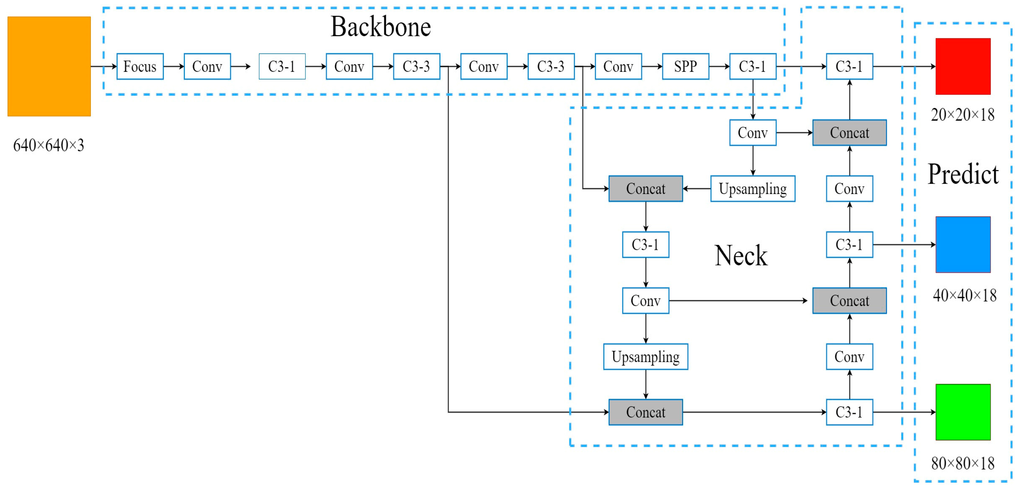
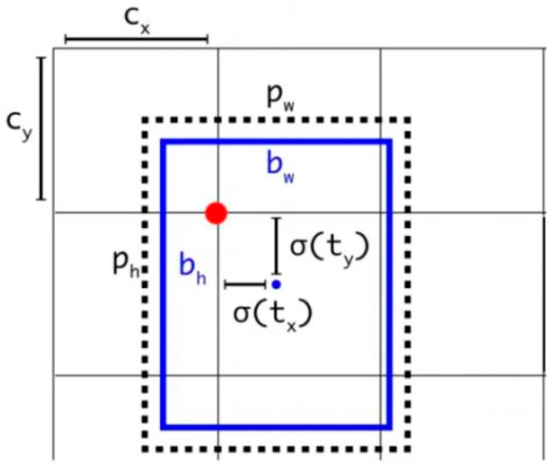
2. Analysis of the Principles Behind the YOLOv5s Algorithm

The YOLO algorithm, proposed by Redmon [21], is a rapid method of object detection. It employs convolutional neural networks (CNNs) to partition the input image into a grid, with each grid cell responsible for detecting whether an object’s center falls within it. Subsequently, the algorithm predicts bounding boxes and their associated confidence scores. Finally, non-maximum suppression is applied to refine the network’s predictions. The currently prevalent YOLO algorithms and their characteristics are compared in

Table 1. Comparison of YOLO algorithm characteristics.

Algorithm
YOLOv3	The introduction of three predictions at different scales enhances small object detection by leveraging both deep and shallow features.
YOLOv4	The introduction of techniques such as the Mish activation function, feature pyramid networks, and adaptive anchor boxes has further enhanced accuracy.
YOLOv5	Using the pytorch framework, we incorporate techniques such as Focus, CSP, and SPP to further enhance accuracy.
YOLOv7	The introduction of transformer modules or similar attention mechanisms has led to the adoption of deeper and more complex network architectures for the extraction of high-level features.
YOLOv8	The C2f module has been utilized, and the incorporation of a decoupled head has significantly enhanced performance.

.

The analysis of the characteristics of various YOLO algorithms listed in Table 1, combined with an examination of their operational mechanisms, reveals that both YOLOv3 and YOLOv4 require a substantial amount of high-quality annotated data during training. This necessity may lead to significant labor costs. Furthermore, it is noted that YOLOv3 exhibits suboptimal performance in detecting partially occluded target objects. The YOLOv5 model employs lightweight network architecture, which maintains a high detection performance while achieving a smaller model size and lower computational resource requirements. The YOLOv7 and YOLOv8 models have made slight adjustments and improvements based on the YOLOv5 framework. They employ relatively deeper and more complex network architectures, resulting in enhanced operational speed. However, as the model size increases, the computation time also rises correspondingly. It is evident that, in model selection, a larger and deeper network structure does not necessarily yield better results. The adaptive image scaling and cross-layer prediction techniques of the YOLOv5 algorithm are particularly well suited for vehicle target detection. Therefore, in this study, the relatively high-precision and lightweight YOLOv5 is selected as the foundation for algorithm improvement. The YOLOv5s algorithm primarily consists of two steps: training and detection. Its network architecture is illustrated in Figure 1, which comprises an input layer (Input), a backbone network (Backbone), a neck component (Neck), a head section (Head), and a prediction module (Predict).

Initially, the input layer resizes the target image to the dimensions required by the model, followed by normalization and data augmentation techniques such as Mosaic enhancement, random flipping, cropping, and color transformation. The processed images are then fed into the Backbone for feature extraction. Subsequently, the Neck integrates these features to enhance their diversity and robustness further. Finally, the Head and Predict modules perform object detection on the obtained feature maps to produce the final output of the network. In Figure 1, “Focus” denotes the attention layer; “Conv” represents the convolutional layer, and “Concat” indicates the concatenation layer. The term “SPP”, or spatial pyramid pooling, refers to the spatial pyramid pooling layer. This algorithm draws on the principles of residual neural networks to address the issue of gradient vanishing that arises with increasing network depth in convolutional networks, thereby enabling deeper propagation within the network.

During the training process, YOLOv5s adopts a novel positive sample selection strategy that differs from previous YOLO algorithms. It is no longer constrained by whether the center point of the ground truth target falls within the grid cell of the feature map. This advancement enables cross-layer predictions; specifically, certain bounding boxes can be considered positive samples across different prediction layers. Each layer is responsible for predicting three bounding boxes of varying sizes. Furthermore, a single target may have multiple anchors assigned to its prediction, thereby increasing the number of positive samples in the network and ultimately leading to an improved object detection model.

During the detection process, YOLOv5s first utilizes a Backbone feature extraction network to output three types of feature maps of different sizes, as illustrated in Figure 2. For instance, when an input image of size 640 × 640 is processed, the dimensions of these three feature maps are as follows: 20 × 20 × 512, 40 × 40 × 256, and 80 × 80 × 128. These feature maps correspond to predictions for large, medium, and small objects, respectively. Subsequently, these three feature maps are fed into a feature fusion network for integration. Finally, through channel adjustment, the network outputs dimensions of 20 × 20 × 18, 40 × 40 × 18, and 80 × 80 × 18. Herein, the numeral 18 represents 3 × (n + 5) and the numeral 3 indicates that each grid cell contains three anchors. The variable n denotes the number of object classes; if there is only one type of target to be recognized, then n takes on the value of 1. The numeral 5 can be expressed as the sum of 4 and 1, and the numeral 1 signifies whether there is an object within that anchor, while the remaining four values represent the predicted bounding box’s offsets relative to the center point of that anchor along with its width and height scaling factors.

The YOLOv5s object detection algorithm based on the anchor initially provides the target’s width and height. However, the model ultimately needs to regress the offset values between the true dimensions of the target and their initial estimates, as well as the relative offsets of the bounding box center with respect to the top-left corner of the grid cell.

To achieve this, it is necessary to process the offset values using the Sigmoid function, as illustrated in Figure 3. In this figure, the dotted box is the anchor, and the blue box is the predicted bounding box, p_w and p_h represent the initial target width and height provided by the anchor, and b_w and b_h denote the true width and height of the target. The variables t_w and t_h correspond to the ratio coefficients of predicted width and height relative to their true values, and t_x and t_y indicate the offsets of the predicted target center point with respect to the grid cell. Additionally, c_x and c_y refer to the coordinates of the top-left corner of the current grid (red dot in Figure 3), whereas b_x and b_y signify the coordinates of the true center point of the target (blue dot in Figure 3). To ensure that the bounding box centers are constrained within their respective grids—thereby guaranteeing that the offset values remain between 0 and 1—the coordinates for each target’s true center can be computed using Equations (1) and (2).

$$b_x=2\sigma \left(t_x\right)-0.5+c_x$$

(1)

$$b_y=2\sigma \left(t_y\right)-0.5+c_y$$

(2)

The actual width and height of the target are calculated using Equations (3) and (4).

$$b_w=p_w{\left(2\sigma \left(t_w\right)\right)}^2$$

(3)

$$b_h=p_h{\left(2\sigma \left(t_h\right)\right)}^2$$

(4)

3. Algorithm Enhancement

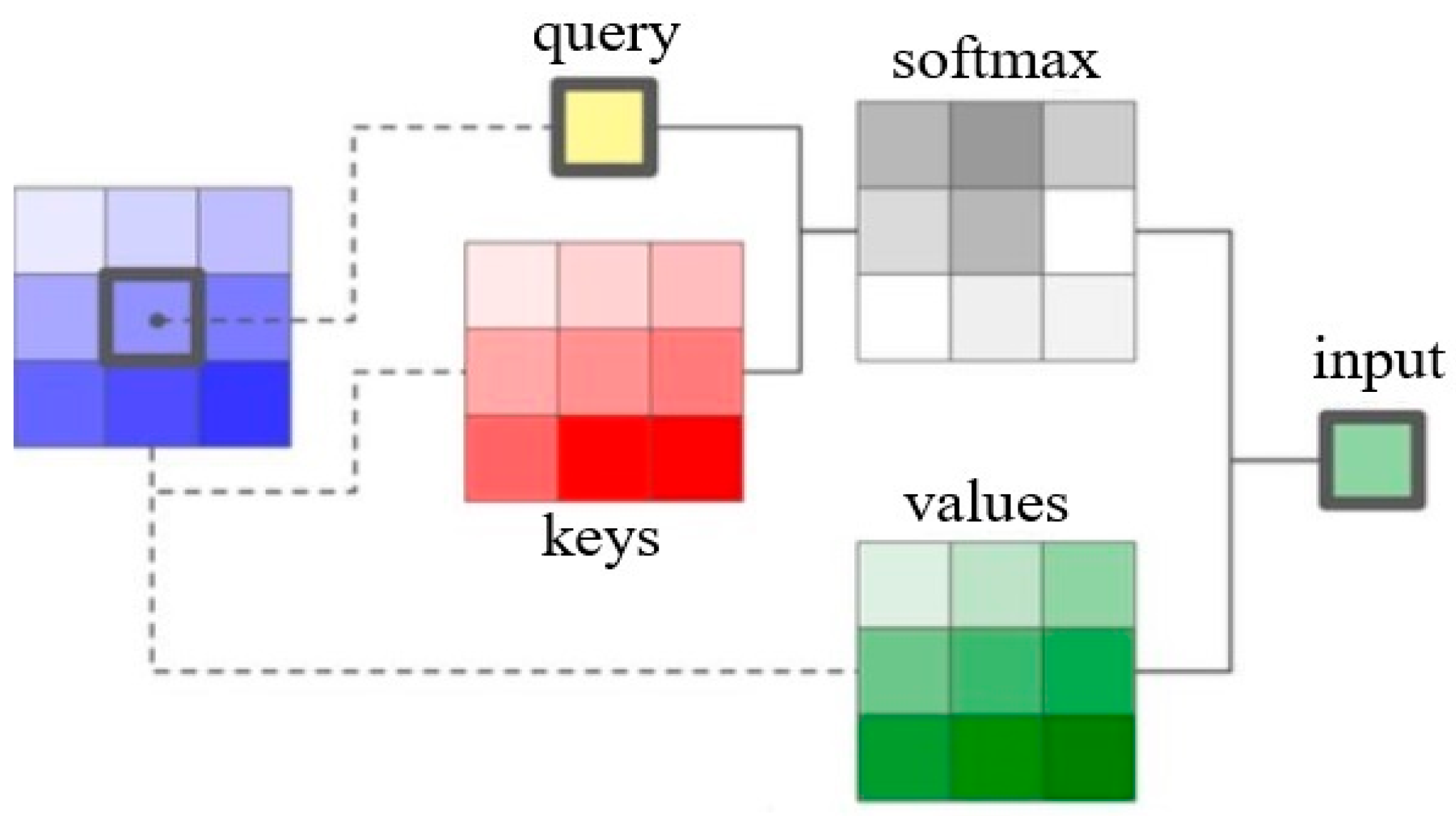
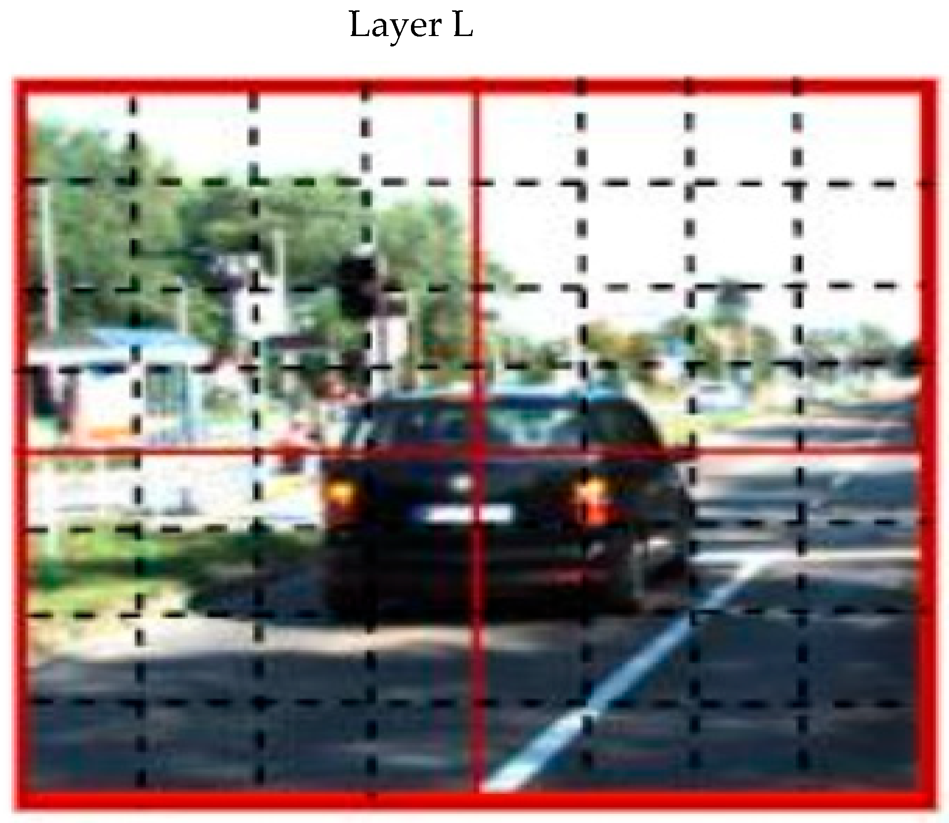
3.1. Introduction of the Swin Transformer Module

Numerous research analyses indicate that convolution operations possess a significant limitation, namely, the ability to extract only local features while missing out on global feature information. To aggregate the locally extracted features from convolutions and obtain deeper semantic representations, it is necessary to construct a model with broader dependencies for object detection tasks. This can be achieved by stacking multiple convolutional layers; however, this approach leads to a substantial increase in computational complexity. To address this limitation, the self-attention mechanism is introduced into computer vision. The visual attention mechanism serves as a unique signal processing method employed by the human brain when processing visual information [22,23,24]. Individuals rapidly scan an overall image with their eyes, swiftly identifying specific areas that warrant closer observation—these become the focal points of attention. Subsequently, they concentrate more cognitive resources on these regions to capture details closely related to the task at hand. In the realm of natural language processing (NLP), self-attention mechanisms facilitate the extraction of contextual information from text, enabling the learning of richer semantic features. The self-attention mechanism is structured into three branches: query, keys, and values. The computation process is illustrated in Figure 4. Initially, the similarity between the query and each key is calculated to obtain weights. These weights are then normalized using the softmax activation function. Finally, the normalized weights are used to perform a weighted sum with their corresponding values associated with the keys, resulting in an output that has been processed through the attention mechanism.

For the self-attention mechanism, the output of each pixel ${\mathrm{y}}_{ij}\in R^{d_{out}}$ can be computed using Equation (5).

$${\mathrm{y}}_{ij}={\displaystyle \sum _{a,bÎN_k(i,j)}softma{x}_{ab}(q_{ij}^T{k}_{ab})n_{ab}}$$

(5)

In the equation, q_ij = W_Qxij, k_ab = W_Kxab, and υ_ab = W_Vxab. The linear variation in pixel points i and j, as well as their surrounding pixel points, is considered. W_Q, W_K, and $W_V\in R^{d_{out}\times d_{in}}$ are the network parameters that require learning within the network.

The Transformer architecture is primarily utilized for natural language processing (NLP) tasks. Due to the differences in scale between the NLP and computer vision domains, the scale in NLP is standardized and fixed. However, the range of scale variations in the field of computer vision is quite extensive. If Transformers are employed within this domain, the computational complexity will be proportional to the square of the image scale, which evidently leads to an excessively large computational burden. To address this issue, Swin Transformer (Swin TR) adopts a hierarchical design approach that begins with smaller windows that progressively increase in size across different layers. This methodology enables the extraction of multi-scale features from images at various levels. Furthermore, incorporating a window mechanism significantly reduces the computational complexity associated with self-attention mechanisms.

The Swin Transformer (Swin TR) consists of two layers of Transformers, namely, standard window attention and shifted window attention, as illustrated in Figure 5 and Figure 6 [25,26]. For the window attention mechanism, the input feature map is first divided into multiple windows. As shown in Figure 5, the red-lined area represents one such window, which contains four distinct windows. Each window comprises several smaller regions referred to as tokens (vectors), indicated by the dashed boxes in Figure 5. Subsequently, all tokens within each individual window are processed using the Transformer architecture; however, there is no information exchange between different windows. Consequently, compared to the original Transformer model, this approach significantly reduces the number of parameters and enhances computational efficiency.

However, the use of a single window attention mechanism can reduce the receptive field of the Transformer, which is detrimental to feature extraction. To address this issue, it was necessary to introduce shift window attention, as illustrated in Figure 6. This approach involved offsetting the windows; for instance, in the second column of the first row, a 2 × 4 window allowed information exchange between two windows in the first row at layer L. Similarly, a 4 × 4 window located in the second column of the second row facilitated communication among four windows at layer L. This method of window shifting effectively resolved the problem of information exchange between different windows. The Swin Transformer employed both window attention and shift window attention by utilizing window attention at layer L and shift window attention at layer L + 1. By implementing this offset technique that enabled inter-window communication, combining layers L and L + 1 satisfies both requirements for an expanded receptive field while simultaneously reducing the parameter count within the Transformer architecture.

3.2. Self-Concat Feature Fusion

Low-level features tend to extract superficial characteristics, such as line color, simple shapes, and basic patterns composed of these simple shapes. Consequently, low-level features are often obtained through a limited number of convolutional operations, resulting in lower semantic significance and higher noise levels. As the depth of the network increases, the semantic richness of the extracted features is enhanced while noise diminishes. However, excessive downsampling due to an increased number of network layers can lead to reduced resolution in feature maps and the loss of detailed information. In light of this issue, fusing both deep and shallow features can effectively enhance the model’s ability to extract information, thereby improving its detection performance.

In YOLOv5s, the feature map concatenation is performed using a simple concatenation (Concat) method. This approach can adversely affect the network’s feature fusion capabilities, resulting in the model’s inability to selectively output more effective feature maps [27,28]. Therefore, during the algorithm improvement process, a weighted feature map concatenation method known as Self-Concat was introduced. Its structure is illustrated in Figure 7.

As can be seen from Figure 7, during the training process, Self-Concat first learns the weight parameters w1 and w2 corresponding to the feature maps x1 and x2, respectively, in order to determine the significance of each feature map. Subsequently, the weighted feature maps are combined through addition and passed through a ReLU activation function for non-linearity. Finally, a 1 × 1 convolution is applied to adjust the number of channels before outputting the result. This approach enables the network to effectively integrate features from different feature maps, thereby enhancing its capacity for feature representation. Based on the principles illustrated in Figure 7, Self-Concat can be formalized as shown in Equation (6).

$$output=conv\left(\delta \left(\underset{i=0}{\overset{1}{cat}}\left(w_i{x}_i\right)\right)\right)$$

(6)

The term w_i is calculated using Equation (7).

$$w_i={\displaystyle \frac{w_i}{{\displaystyle \sum _{j=0}^1{w}_j}}}+\xi$$

(7)

In the above two equations, δ represents the ReLU activation function; w_i and w_j denote the predictive weights of the network; and ζ is a small, fixed value introduced to prevent division by zero.

According to Equation (6), during the training process, if a feature x_i significantly contributes to the final predictions of the network, the network will automatically assign a larger weight to that feature. Conversely, if a feature contributes less, the network will allocate a smaller weight to it. This process is entirely determined by the training procedure and occurs without any human intervention.

For Equation (6), the backpropagation process is implemented using the chain rule. The derivation of w_i is illustrated in Equation (8).

$${\displaystyle \frac{\mathit{\partial }O}{\mathit{\partial }{\mathrm{w}}_i}}={\displaystyle \frac{\mathit{\partial }O}{\mathit{\partial }conv}}{\displaystyle \frac{\mathit{\partial }conv}{\mathit{\partial }relu}}{\displaystyle \frac{\mathit{\partial }relu}{\mathit{\partial }cat}}{\displaystyle \frac{\mathit{\partial }cat}{\mathit{\partial }{\mathrm{w}}_i}}$$

(8)

In the equation, ${\displaystyle \frac{\mathit{\partial }O}{\mathit{\partial }conv}}$, ${\displaystyle \frac{\mathit{\partial }conv}{\mathit{\partial }relu}}$, and ${\displaystyle \frac{\mathit{\partial }relu}{\mathit{\partial }cat}}$, respectively, represent the gradients of the convolution operation, the gradient of the ReLU activation function, and the gradient of the concatenation operation. Based on established methods for solving these three known gradients, we can further simplify the gradient with respect to w_i, as shown in Equation (9).

$${\displaystyle \frac{\mathit{\partial }O}{\mathit{\partial }{\mathrm{w}}_i}}={\displaystyle \frac{\mathit{\partial }O}{\mathit{\partial }conv}}{\displaystyle \frac{\mathit{\partial }conv}{\mathit{\partial }relu}}{\displaystyle \frac{\mathit{\partial }relu}{\mathit{\partial }cat}}{x}_i$$

(9)

From Equation (9), it can be observed that the Self-Concat concatenation method simplifies the gradient computation process. Furthermore, based on the gradient descent algorithm, it allows for continuous updates of w_i during the training process.

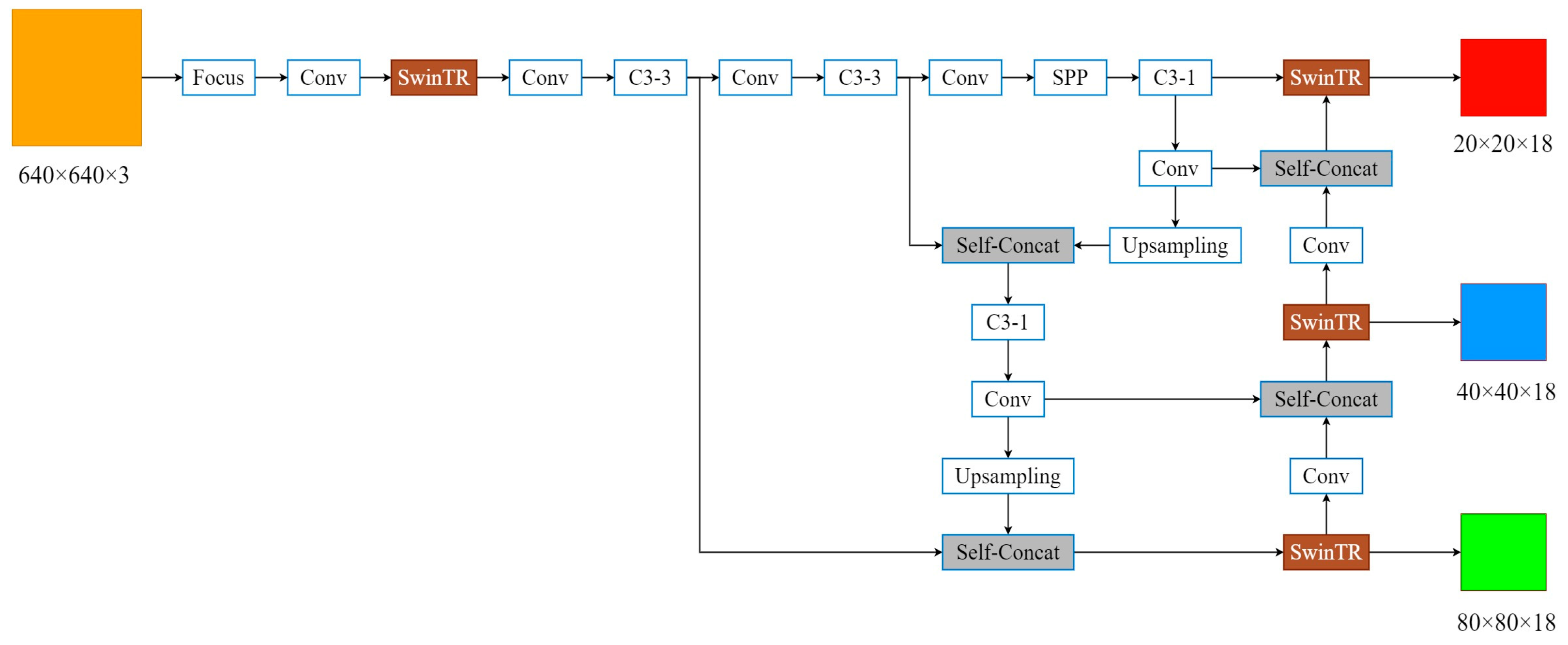
3.3. Improved Structure of the Swin-YOLOv5s Algorithm

In order to further enhance the detection speed and accuracy of the model, we conducted an analytical investigation into the principles of the YOLOv5s algorithm. Consequently, the novel vehicle target detection algorithm based on Swin Transformer was proposed—Swin-YOLOv5s. The algorithm introduces the Swin Transformer as one of the layers within the YOLOv5s network structure without altering the overall architecture. The modified network structure is illustrated in Figure 8. In this improvement, the third layer of the Backbone network in the original YOLOv5s is replaced with a Swin TR module to enhance the receptive field of the network, enabling it to extract more comprehensive and richer features from targets. Subsequently, to capture holistic feature information from the three feature maps generated by the network, the existing C3-1 network structure in the feature fusion section is also substituted with a Swin TR module, further enhancing the model’s capability for feature extraction. In addition, to enhance the feature fusion capability of the network, we optimized the Concat module based on the existing FPN + PAN network structure and introduced a novel feature fusion method called Self-Concat. This approach integrates features from different levels through a weighted mechanism, allowing the network to adaptively adjust the weights corresponding to various feature maps. Consequently, this method aims to suppress the negative features of the target while enhancing its positive characteristics.

The introduction of the Swin-Transformer network architecture (Swin TR module) and the feature fusion structure (Self-Concat module), as illustrated in Figure 8, significantly enhance the network’s capabilities for feature extraction and fusion. This overall improvement contributes to an increase in the model’s detection accuracy. Furthermore, the sliding window mechanism incorporated within the Swin TR effectively reduces computational load, thereby facilitating faster detection speeds compared to traditional Transformers.

4. Experimental Analysis and Validation

4.1. Dataset and Experimental Environment

The KITTI benchmark dataset, which is currently the most widely used in the context of autonomous driving scenarios, is based on real-world scenes and encompasses a variety of environments including urban areas, rural settings, and highways [29,30]. The most complex images within this dataset feature up to 15 vehicles and 30 pedestrians. Additionally, these images exhibit varying degrees of road occlusion or wear. The image resolution is set at 1392 × 512 pixels. The data categories include cars, vans, trucks, pedestrians on the road, individuals resting, cyclists, trams, and several other objects. Due to the focus of this study on vehicle object detection, cars, vans, and trucks in the dataset were uniformly consolidated into a single category labeled “cars”. A total of 6798 images containing vehicles were extracted from the dataset. Subsequently, these images were randomly divided into a training set comprising 5778 images and a validation set consisting of 1020 images. Experiments were conducted using this dataset to compare the algorithmic performance of the two models before and after improvements. To mitigate potential impacts on the model training and the inference speed due to the suboptimal performance of standard graphics cards, high-performance servers were utilized for experimentation. The hardware configuration included a Windows 10 operating system; Intel(R) Core(TM) i7-10875H CPU (Intel Corp., Santa Clara, CA, USA); Tesla V100 GPU with a greater number of computing units and a larger memory capacity; 32 GB RAM; and PyTorch 2.0.1 serving as the deep learning framework and programming carried out in Python 3.7. The hyperparameter settings employed during the experiments are detailed in

Table 2. Configuration of experimental parameters.

Parameter	Initialize Learning Rate	Momentum	Weight Decay	Refinement of Training Epochs	Batch Size	Image Size	Learning Rate Decay Strategies
Value	0.001	0.937	0.0005	120	50	640 × 640	cosine

. The initial learning rate, momentum, and weight decay were all set to their default values. To ensure that the model had an appropriate learning rate at different stages of training and to facilitate rapid exploration in the early phase followed by precise fine-tuning in the later phase—thereby accelerating both convergence speed and detection accuracy—we employed cosine annealing for learning rate adjustment. The batch size and number of training epochs were determined through multiple experiments to ensure convergence.

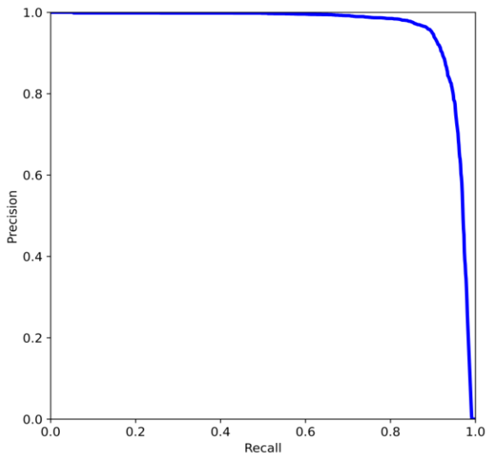
4.2. Performance Evaluation Metrics

In the context of object detection algorithms, evaluation metrics such as precision (P), recall (R), F1 score, mean average precision (mAP) for multi-class scenarios, and frames per second (FPS) are employed to conduct comparative analyses of experimental results. Each metric serves to characterize the performance of the detection model to a certain extent. By comparing these metrics across different models, one can discern their respective strengths and weaknesses [31,32]. Precision (P) is defined as the ratio of true positive predictions among all predicted positive samples. Recall (R) represents the ratio of true positive predictions among all actual positive samples.

However, the use of precision or recall alone is insufficient to evaluate the performance of a model. Therefore, combining precision and recall yields two additional metrics: the F1 score and the mean average precision (mAP). The mAP serves as a universal metric for object detection, representing the average of the average precision (AP) values across multiple categories. Each category’s AP is calculated based on the area under the curve formed by P and R. The calculations for precision and recall are provided in Equations (10) and (11), respectively.

$$Precesion={\displaystyle \frac{\mathrm{TP}}{\mathrm{TP}+\mathrm{FP}}}$$

(10)

$$Recall={\displaystyle \frac{\mathrm{TP}}{\mathrm{TP}+\mathrm{FN}}}$$

(11)

In the formulae, TP represents the true positive, indicating the correct detection of positive samples; FP denotes the false positive, signifying an incorrect detection of negative samples as positive; and FN refers to the false negative, representing a failure to detect positive samples.

The curve obtained by plotting precision on the vertical axis and recall on the horizontal axis is known as the PR curve. The PR curve serves as one of the important metrics for evaluating model performance. By utilizing the PR curve, it is possible to calculate the average precision (AP) value according to Formula (12), which can be employed to assess the detection effectiveness of the model.

$$AP={\displaystyle {\int }_0^{1}p\left(r\right)}dr$$

(12)

The calculation formula for mAP is presented in Equation (13). The mean average precision (mAP) represents the average area enclosed by multiple class PR curves and the coordinate axes. In this study, during data processing, cars, vans, and trucks were combined into a single category; therefore, there was only one type of vehicle model considered. As a result, the AP value was equal to the mAP value.

$$mAP={\displaystyle \frac{1}{classes}}{\displaystyle \sum _{i=1}^{classes}{\displaystyle {\int }_0^{1}p\left(r\right)}dr}$$

(13)

The results of F1 are calculated using Equation (14).

$$F1={\displaystyle \frac{2\times Precision\times Recall}{Precision+Recall}}$$

(14)

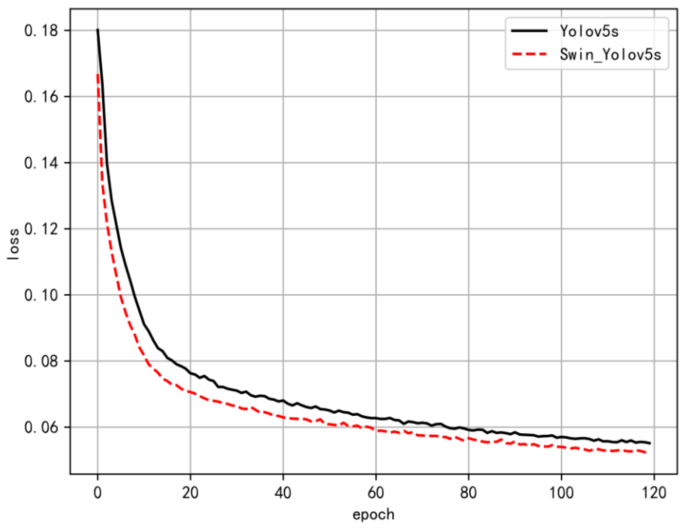
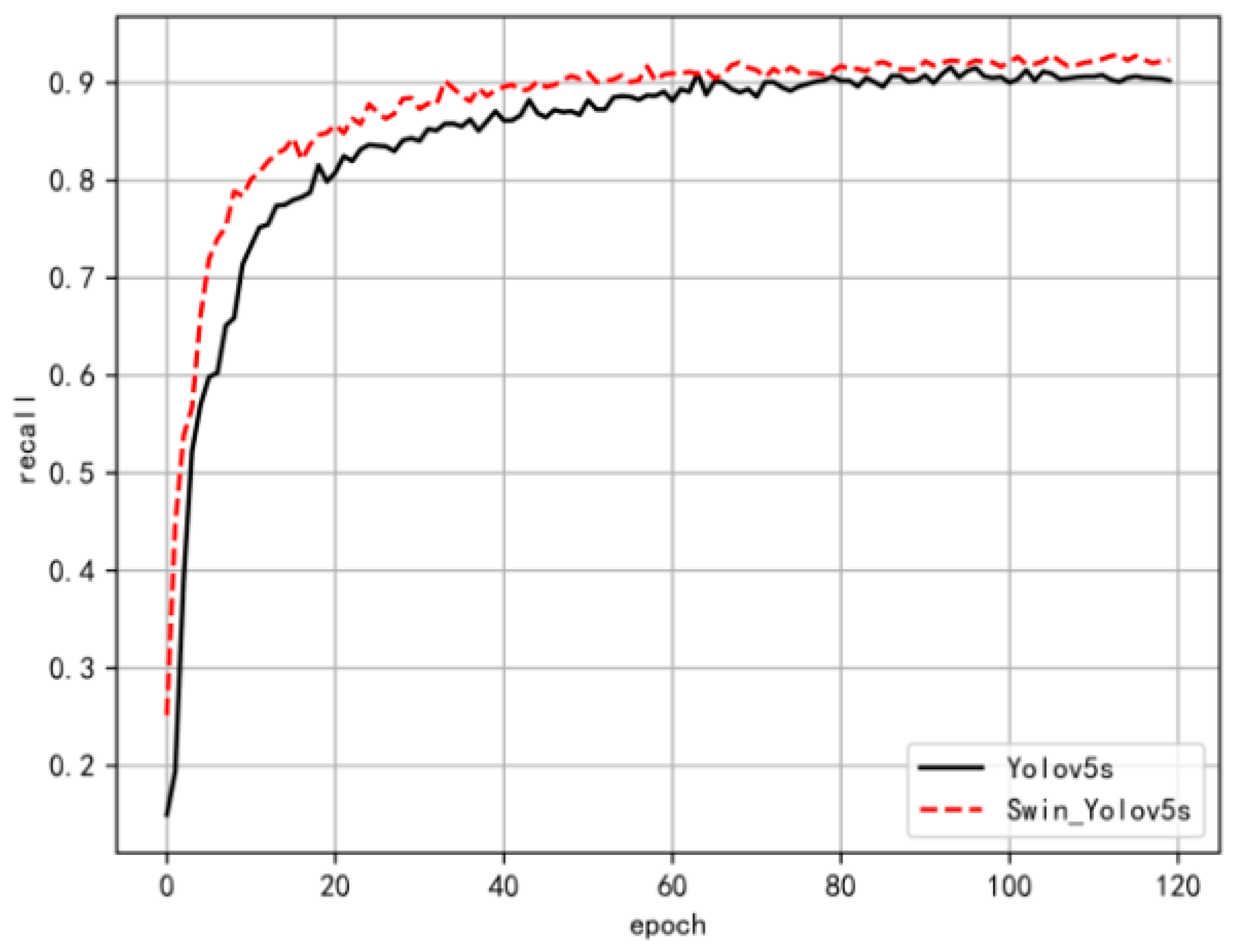
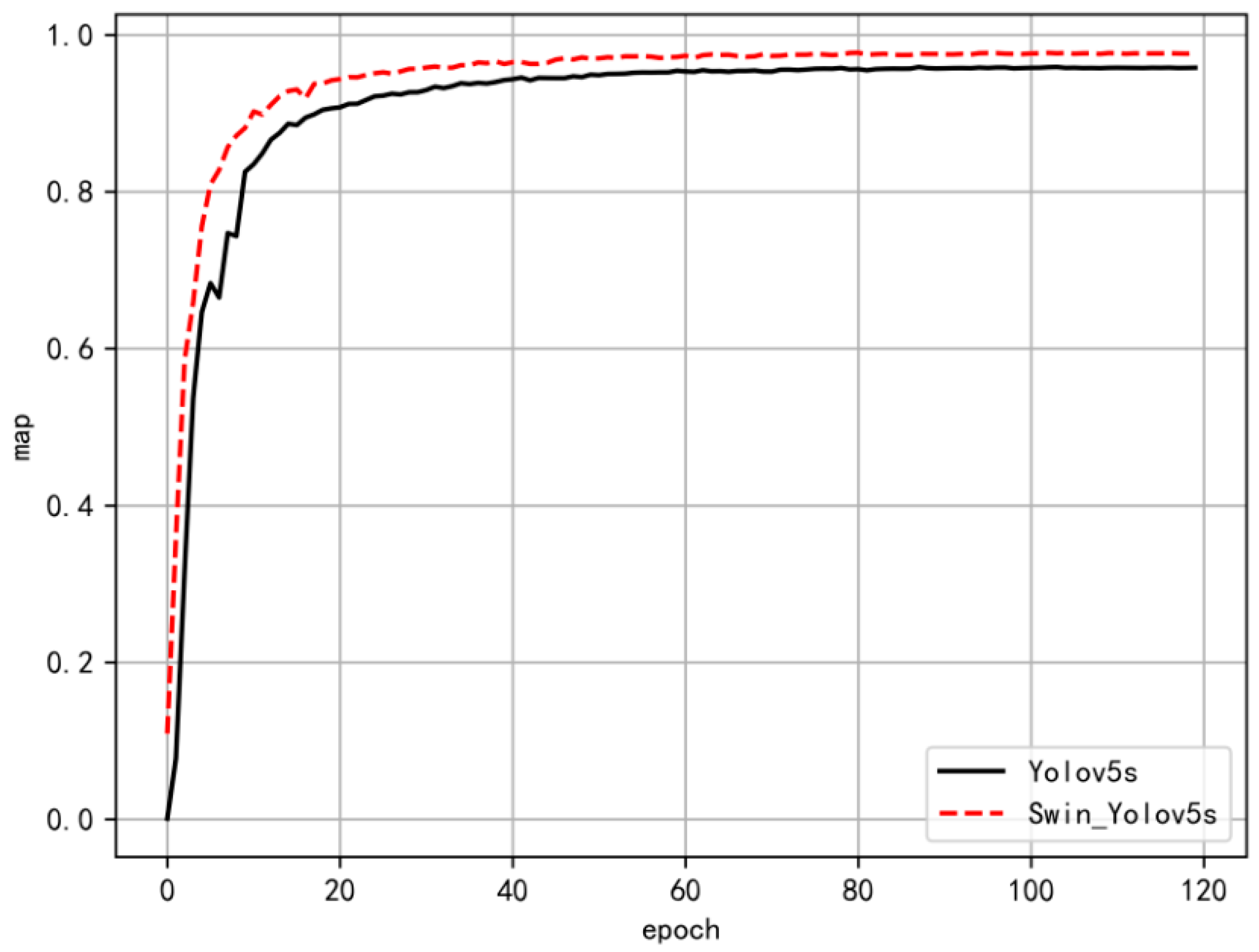
4.3. Experimental Validation and Analysis

In the same experimental environment and using the same dataset, both YOLOv5s and Swin-YOLOv5s underwent training. Subsequently, the performance of the models on the validation set based on various metrics were compared, including accuracy, recall, F1 score, mAP, and detection speed. The models before and after improvement underwent 120 iterations of training. During the training process, the loss values for each epoch were recorded, resulting in the final loss function curves for both models, as illustrated in Figure 9.

The loss curves indicate that both YOLOv5s and Swin-YOLOv5s exhibit a rapid decrease in loss during the initial stages of training. Specifically, from epochs 0 to 40, it is evident that Swin-YOLOv5s demonstrates a more pronounced downward trend in loss compared to YOLOv5s. From epoch 40 to 120, the losses for both models continue to decline gradually; by epoch 100, they stabiliz and approach convergence. Notably, the overall loss of Swin-YOLOv5s is lower than that of YOLOv5s throughout this period. Since the magnitude of the loss value reflects the proximity between the ground truth and bounding boxes, it can be concluded that Swin-YOLOv5s exhibits superior detection performance relative to YOLOv5s.

During the model training process, a comparative analysis of precision (P) and recall (R) was conducted. The corresponding curves are illustrated in Figure 10 and Figure 11.

According to Figure 10 and Figure 11, during the training process over 120 iterations, Swin-YOLOv5s demonstrates a notable improvement in both accuracy and recall compared to YOLOv5s. This indicates that Swin-YOLOv5s is capable of making more effective inferences, resulting in enhanced performance regarding accuracy and recall. However, evaluating model performance solely based on precision and recall does not provide a comprehensive assessment; it is essential to analyze the mAP variation curves for both models, as illustrated in Figure 12.

As seen in Figure 12, Swin-YOLOv5s demonstrates a notable improvement in mAP values compared to YOLOv5s. It is important to note that the mAP is related to both accuracy and recall. This observation supports the conclusions drawn from Figure 10 and Figure 11, indicating that Swin-YOLOv5s exhibits enhancements in both precision and recall relative to YOLOv5s.

The PR curves of the model before and after improvement on the KITTI validation set are presented in Figure 13 and Figure 14. From these figures, it is evident that the overall trend of the PR curve exhibits a decreasing pattern. This phenomenon can be attributed to the inherent trade-off between precision and recall; it is impossible for both metrics to achieve their maximum values simultaneously. When striving for higher precision, there tends to be a corresponding decline in recall, and vice versa.

The area under the PR curve is referred to as the AP value and can be used to assess the performance of a model in vehicle detection. When this area approaches 1, it indicates that the model is capable of detecting vehicles within images and accurately identifying their respective locations, reflecting a strong performance. Conversely, when the area approaches 0, it signifies that the model fails to detect vehicles in the images and cannot locate their positions, indicating poor performance. By examining both PR curves, it is evident that the AP value for Swin-YOLOv5s significantly exceeds that of YOLOv5s. Therefore, it can be concluded that the improved Swin-YOLOv5s model demonstrates superior detection capabilities compared to the traditional YOLOv5s.

In order to further evaluate the performance of the improved Swin-YOLOv5s model, the mean average precision (mAP) and the F1 scores of both the modified Swin-YOLOv5s model and the original YOLOv5s model were compared using the validation set from KITTI. Due to data preprocessing, which merged three types of vehicles into one category, the mAP values were equivalent to their corresponding average precision (AP) values. When there was little difference between the mAP values of both models, additional evaluation could be conducted through the F1 results. The findings are presented in

Table 3. Comparison of overall metrics before and after model improvement.

Model	mAP@0.5 (%)	F1 (%)	Precision (%)	Recall (%)	Time Consumption for a Single Image (ms)	Detection Speed (FPS)
Swin-YOLOv5s	95.7	93.01	96.02	90.24	3.2	312.5
YOLOv5s	94.1	92.45	95.51	89.62	3.6	277.7

.

As seen in Table 2, the mAP of the improved Swin-YOLOv5s is 95.7%, representing an enhancement of 1.6% over YOLOv5s. Additionally, the F1 score for Swin-YOLOv5s is 93.01%, which indicates an increase of 0.56% compared to YOLOv5s. Considering these two evaluation metrics comprehensively, it can be concluded that the detection performance of Swin-YOLOv5s surpasses that of YOLOv5s. Furthermore, it can also be observed from Table 3 that, when tested on the Tesla V100, the inference speed of the Swin-YOLOv5s is 3.2 ms per image, while YOLOv5s has an inference speed of 3.6 ms per image. This demonstrates a reduction in inference time and an improvement in inference speed of 1.11%. In terms of frames per second (FPS), the Swin-YOLOv5s shows an increase of 34.8 FPS compared to YOLOv5s, representing an increase of 12.5%. These findings suggest that the proposed Swin-YOLOv5s algorithm not only enhances the mAP value of the YOLOv5s model but also significantly accelerates the detection speed. Therefore, it can be concluded that Swin-YOLOv5s is well suited for vehicle detection in road scenarios.

In order to validate the effectiveness of the improvements made to the Swin-YOLOv5s algorithm, three groups of ablation experiments were designed under identical experimental conditions. The results are presented in

Table 4. Comparison of ablation experiment.

Algorithm	Swin TR	Self-Concat	Parameter Count (M)	GFLOPS	mAP@0.5 (%)	Time Consumption for a Single Image (ms)	FPS
1	×	×	7.31	51.5	94.1	3.6	277.7
2	√	×	5.63	30.4	95.2	3.2	296.4
3	√	√	5.03	21.8	95.7	3.2	312.5

. In this table, “√” indicates the use of improved methods, while “×” signifies that no improvements were applied.

As seen in Table 4, replacing the C3-1 module in the Backbone network with the Swin Transformer (Swin TR) leads to a reduction of approximately 23% in computational complexity due to the introduction of a window mechanism. This modification results in an improvement in both detection speed and frames per second. Furthermore, by employing a dynamically allocated weight Self-Concat instead of the simple concatenation method (Concat), we observe an additional decrease in computational load, with floating-point operations reduced by approximately 5.8% compared to the original algorithm. These enhancements demonstrate that our proposed algorithm improves detection accuracy and speed without compromising computational efficiency, thereby validating the effectiveness of our improvements.

In order to further compare the effectiveness of the improved algorithm, comparative experiments were conducted under identical conditions using the same training strategies and equipment. The results are presented in

Table 5. Comparison of different network models in experimental studies.

Algorithm	Precision (%)	Recall (%)	mAP@0.5 (%)	F1 (%)	Parameter Count (M)
YOLOv3	92.94	86.83	92.1	89.78	61.56
YOLOv3-Tiny	89.73	68.81	78.5	77.89	8.63
YOLOv7	95.72	84.75	95.5	89.90	20.94
Faster R-CNN	96.66	90.57	96.3	93.52	38.4
YOLOv5s	95.51	89.62	94.1	92.45	7.31
Swin-YOLOv5s	96.02	90.24	95.7	93.01	5.03

.

The experimental results indicate that the performance of the YOLOv3 algorithm is inferior to that of the YOLOv5s algorithm, which also has a larger number of parameters. When comparing the YOLOv5s algorithm to YOLOv7 under identical conditions, there is a significant reduction in parameter count along with improvements in F1 and recall metrics, while other indicators remain relatively close. Although the Faster R-CNN algorithm shows certain enhancements over the Swin-YOLOv5s algorithm across various metrics, its two-stage detection principle leads to an increase in computational parameters by 33.37 M. Furthermore, the improved Swin-YOLOv5s algorithm outperforms YOLOv3, YOLOv3-Tiny, YOLOv7, and YOLOv5s across all five evaluated metrics. While it exhibits comparable precision and mAP values relative to YOLOv7, it achieves notable increases in recall and F1 scores by 6.5% and 3.5%, respectively. Additionally, there is a reduction of 15.9 M in parameter count, significantly lowering computational complexity.

To provide a more intuitive comparison between the detection performance of Swin-YOLOv5s and YOLOv5s, we conducted image detections on the test set, with the results illustrated in Figure 15 and Figure 16, respectively.

Figure 15 shows that the Swin-YOLOv5s algorithm achieves confidence scores of 0.926 and 0.947 when detecting the white and black vehicles, respectively. These scores are significantly higher than those obtained by the YOLOv5s algorithm, with recorded values of 0.911 and 0.904 for the same tasks. A similar trend is evident in Figure 16, further demonstrating that the improved Swin-YOLOv5s algorithm outperforms YOLOv5s in detection efficacy. In examining Figure 16, it is noted that there is a vehicle located to the left front of the current black vehicle, as indicated by the red arrow. Although this vehicle is substantially obscured by another, the application of the Swin-YOLOv5s algorithm still enables effective detection. In contrast, when faced with this scenario, the YOLOv5s algorithm exhibits instances of missed detections. This improvement can be attributed to the enhanced global information capture capability inherent in the modified Swin-YOLOv5s algorithm.

5. Conclusions

(1)

In response to the issues of low detection accuracy, slow speed, and high rates of false positives and missed detections in the existing YOLOv5s vehicle detection model, an improved Swin-YOLOv5s vehicle target detection algorithm was proposed by incorporating a Swin Transformer attention mechanism along with a novel feature fusion approach based on Self-Concat. The proposed algorithm was capable of extracting vehicle information at a deeper level and adaptively adjusting the weights of feature maps to suppress the negative characteristics of the target.

(2)

The proposed algorithm was effectively trained and tested using the KITTI dataset. The improved Swin-YOLOv5s model achieved a 1.6% increase in mean average precision compared to the YOLOv5s model, along with a 0.56% enhancement in the F1 score. Additionally, the inference speed for a single image increased by 1.11%, while the overall detection speed measured in frames per second (FPS) improved by 12.5%. The ablation experiments and comparative experiments with various network models both validated the efficiency and accuracy of this model, which also demonstrated strong generalization capabilities and rapid detection speeds.

(3)

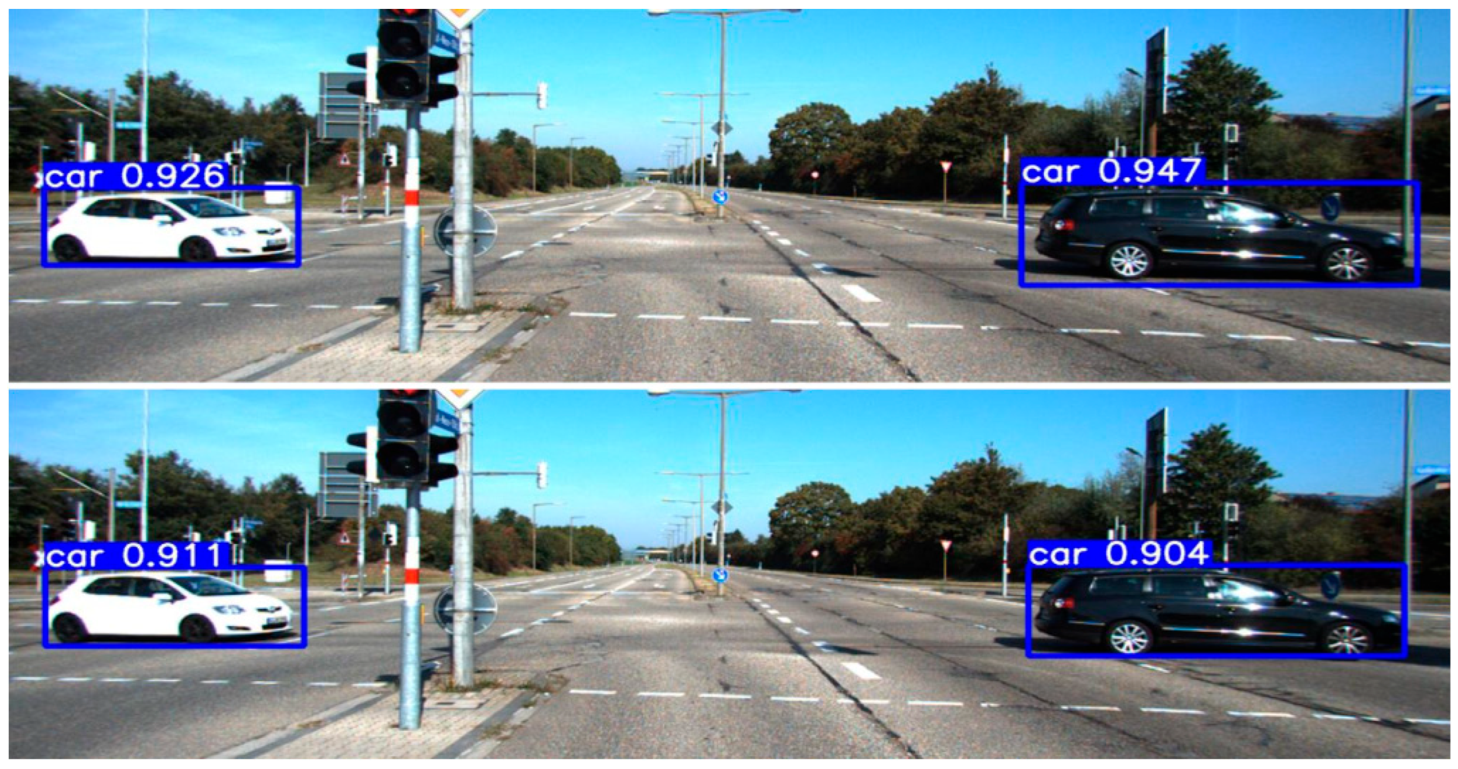
The results of the test set image detection indicated that the proposed Swin-YOLOv5s vehicle detection algorithm demonstrated a significantly higher confidence level across various scenarios compared to the YOLOv5s algorithm. Furthermore, even in cases of severe vehicle occlusion, it maintained effective detection capabilities, thereby addressing the issue of missed detections inherent to the YOLOv5s algorithm.

(4)

In future research, it is essential to test the algorithm on various hardware platforms. Additionally, training and validation should be conducted using other datasets as well as self-constructed augmented datasets under diverse conditions. Furthermore, comparisons with more advanced network models are necessary for improvement, aiming to enhance the effectiveness of this method.

References

1. Khan, S.K.; Shiwakoti, N.; Stasinopoulos, P.; Chen, Y.L.; Warren, M. The impact of perceived cyber-risks on automated vehicle acceptance: Insights from a survey of participants from the United States, the United Kingdom, New Zealand, and Australia. Transp. Policy 2024, 152, 87–101. [Google Scholar]
2. Bengamra, S.; Mzoughi, O.; Bigand, A.; Zagrouba, E. A comprehensive survey on object detection in Visual Art: Taxonomy and challenge. Multimed. Tools Appl. 2023, 83, 14637–14670. [Google Scholar] [CrossRef]
3. Xiao, Z.; Luo, L.; Chen, M.; Wang, J.; Lu, Q.; Luo, S. Detection of grapes in orchard environment based on improved YOLO-V4. J. Intel. Agri. Mech. 2023, 4, 35–43. [Google Scholar]
4. Mozumder, M.; Biswas, S.; Vijayakumari, L.; Naresh, R.; Kumar, C.N.S.V.; Karthika, G. An Hybrid Edge Algorithm for Vehicle License Plate Detection. In Proceedings of the International Conference on Intelligent Sustainable Systems, Bangalore, India, 26–27 September 2023; Springer: Singapore, 2023. [Google Scholar]
5. Mei, S.; Ding, W.; Wang, J. Research on the real-time detection of red fruit based on the you only look once algorithm. Processes 2024, 12, 15. [Google Scholar]
6. Dai, Y.; Fang, X. An armature defect self-adaptation quantitative assessment system based on improved YOLO11 and the degment anything model. Processes 2025, 13, 532. [Google Scholar]
7. Othman, K.M.; Alfraihi, H.; Nemri, N.; Miled, A.B.; Alruwais, N.; Mahmud, A. Exploiting remote sensing imagery for vehicle detection and classification using robust competitive algorithm with deep convolutional neural network. Fractals 2024, 32, 1–16. [Google Scholar]
8. Sivaraman, S.; Trivedi, M.M. Looking at vehicles on the road: A survey of vision-based vehicle detection, tracking, and behavior analysis. IEEE Trans. Intell. Transp. Syst. 2013, 14, 1773–1795. [Google Scholar]
9. Tang, M.J.; Cai, S.F.; Lau, V.K.N. Over-the-Air aggregation with multiple shared channels and graph-based state estimation for industrial IoT systems. IEEE Internet Things J. 2021, 8, 14638–14657. [Google Scholar] [CrossRef]
10. Geetha, A.S. Comparing YOLOv5 variants for vehicle detection: A Performance Analysis. arXiv 2024, arXiv:2408.12550. [Google Scholar]
11. Bakirci, M. Real-time vehicle detection using YOLOv8-nano for intelligent transportation systems. Trait. Signal 2024, 41, 1727. [Google Scholar] [CrossRef]
12. Vasavi, S.; Raj, G.H.; Suhitha, T.S. Onboard processing of drone imagery for military vehicles classification using enhanced YOLOv5. J. Adv. Inf. Technol. 2023, 14, 1221–1229. [Google Scholar]
13. Hao, Y.; Geng, C. Improved pedestrian vehicle detection for small objects based on attention mechanism. Int. J. Adv. Netw. Monit. Control. 2024, 9, 80–89. [Google Scholar] [CrossRef]
14. Hong, T.S.; Ma, Y.J.; Jiang, H. Vehicle identification and analysis based on lightweight YOLOv5 on edge computing platform. Meas. Sci. Technol. 2025, 36, 16–44. [Google Scholar] [CrossRef]
15. Wang, C.L.; Zhou, Y.Q.; Lv, Z.G.; Ye, C.Q.; Xiang, X.J. Research on tunnel vehicle detection based on GCM-YOLOv5s. J. Beijing Jiaotong Univ. 2025, 2, 1–16. [Google Scholar]
16. Deng, C.; Ma, J.J.; Yan, Y.; Wang, Y.F.; Li, Y.Q. Vehicle identification algorithms based on lightweight neural networks. J. Chongqing Jiaotong Univ. 2024, 43, 80–87. [Google Scholar]
17. Hu, P.F.; Wang, Y.G.; Zhai, Q.Q.; Yan, J.; Bai, Q. Night vehicle detection algorithm based on YOLOv5s and bistable stochastic resonance. Comput. Sci. 2024, 51, 173–181. [Google Scholar]
18. Zhao, L.L.; Wang, X.Y.; Zhang, Y.; Zhang, M.Y. Vehicle target detection based on YOLOv5s fusion SENet. J. Graph. 2022, 43, 776–782. [Google Scholar]
19. Fan, J.X.; Zhang, W.H.; Zhang, L.L.; Yu, T.; Zhong, L.C. Vehicle detection method of UAV imagery based on improved YOLOv5. Remote Sens. Inf. 2023, 38, 114–121. [Google Scholar]
20. Chen, D.D.; Ren, X.M.; Li, D.P.; Chen, J. Research on binocular vision vehicle detection and ranging method based on improved YOLOv5s. J. Optoelectron. Laser 2024, 35, 311–319. [Google Scholar]
21. Mishra, S.; Yadav, D. Vehicle detection in high density traffic surveillance data using YOLO.v5. Recent Adv. Electr. Electron. Eng. 2024, 17, 216–227. [Google Scholar] [CrossRef]
22. Wu, C.x.; Hu, J. Efficient image super-resolution reconstruction via symmetric visual attention network. Softw. Guide 2025, 2, 1–6. [Google Scholar]
23. Jiang, T.Y.; Hu, C.J.; Zheng, L.Z. Cable detection method with modified DeepLabV3+ network based on attention mechanism. J. Transp. Sci. Eng. 2025, 2, 1–11. [Google Scholar]
24. Wang, K.; Chen, H.; Chen, L.M.; Huang, H.P.; Chen, X.L. Two-stage point cloud reconstruction based on improved attention mechanism and surface differential geometry. ACTA Metrol. Sin. 2024, 45, 952–963. [Google Scholar]
25. Hüseyin, F.; Hüseyin, Z.; Atila, O.; Engür, A. Automated efficient traffic gesture recognition using swin transformer-based multi-input deep network with radar image. Signal Image Video Process. 2025, 19, 1–11. [Google Scholar]
26. Tayaranian, M.; Mozafari, S.H.; Clark, J.J.; Meyer, B.; Gross, W. Faster inference of integer SWIN transformer by removing the GELU activation. arXiv 2024, arXiv:2402.01169. [Google Scholar]
27. Subburaj, K.; Mazroa, A.A.; Alotaibi, F.A.; Alnfiai, M.M. DBCW-YOLO: An advanced yolov5 framework for precision detection of surface defects in steel. Matéria 2024, 29, e20240549. [Google Scholar]
28. Vítor, C. A Novel Deep Learning Approach for Yarn Hairiness Characterization Using an Improved YOLOv5 Algorithm. Appl. Sci. 2024, 15, 149. [Google Scholar] [CrossRef]
29. Qureshi, A.M.; Butt, A.H.; Alazeb, A.; Mudawi, N.A.; Alonazi, M.; Almujally, N.A.; Jalal, A.; Liu, H. Semantic segmentation and YOLO detector over aerial vehicle Images. Comput. Mater. Contin. 2024, 80, 3315–3332. [Google Scholar]
30. Abdallah, S.M. Real-time vehicles detection using a tello drone with YOLOv5 algorithm. Cihan Univ.-Erbil Sci. J. 2024, 8, 1–7. [Google Scholar]
31. Lv, J.M.; Zhang, F.; Luo, Y.B. Improved YOLOv5s based target detection algorithm for tobacco stem material. J. Zhejiang Univ. 2024, 58, 2438–2446. [Google Scholar]
32. Tian, D.; Wei, X.; Yuan, J. Vehicle target detection algorithm based on improved YOLOv5 lightweight. Comput. Appl. Softw. 2024, 41, 240–246. [Google Scholar]
Figure 1. YOLOv5s structure diagram.
Processes 13 00925 g001
Figure 2. Schematic diagram of the YOLOv5s detection network.
Processes 13 00925 g002
Figure 3. Preprocessing of the YOLOv5s prediction structure encoding using the sigmoid function.
Processes 13 00925 g003
Figure 4. Self-attention mechanism.
Processes 13 00925 g004
Figure 5. Window attention.
Processes 13 00925 g005
Figure 6. Shift window attention.
Processes 13 00925 g006
Figure 7. Self-Concat structure diagram.
Processes 13 00925 g007
Figure 8. Swin-YOLOv5s structural diagram.
Processes 13 00925 g008
Figure 9. Swin-YOLOv5s and YOLOv5s model training process loss curve.
Processes 13 00925 g009
Figure 10. Comparison of precision curves.
Processes 13 00925 g010
Figure 11. Comparison of recall curves.
Processes 13 00925 g011
Figure 12. The mAP variation curve of Swin-YOLOv5s and YOLOv5s models.
Processes 13 00925 g012
Figure 13. Swin-YOLOv5s precision–recall curve.
Processes 13 00925 g013
Figure 14. YOLOv5s precision–recall curve.
Processes 13 00925 g014
Figure 15. The detection performance of Swin-YOLOv5s (top) and YOLOv5s (bottom).
Processes 13 00925 g015
Figure 16. The detection performance of Swin-YOLOv5s (top) and YOLOv5s (bottom) in the presence of occlusion.
Processes 13 00925 g016