A Position–Force Feedback Optimal Control Strategy for Improving the Passability and Wheel Grounding Performance of Active Suspension Vehicles in a Coordinated Manner

Abstract

This paper aims to solve the problems of poor mobility, passability, and stability in heavy-duty vehicles, and proposes an active suspension system control strategy based on position–force feedback optimal control to coordinately enhance vehicle passability and wheel grounding performance. Firstly, a two-degrees-of-freedom one-sixth vehicle active suspension model and a valve-controlled hydraulic actuator system model are constructed, and the advantages of impedance control in robot compliance control are integrated to analyze their applicability in hydraulic active suspension. Next, a position feedback controller and force feedback LQG optimal controller for fuzzy PID control are designed, the fuzzy PID-LQG (FPL) integrated method is applied to the hydraulic active suspension system, and the dynamic load of the wheel is tracked by impedance control to obtain the spring mass displacement correction. Then, a suspension system model under the excitation of a C-class road surface and a 0.11 m raised road surface is constructed, and the dynamic simulation and comparison of active/passive suspension systems are carried out. The results show that, compared with PS and LQR control, the body vertical acceleration, suspension dynamic deflection, and wheel dynamic load root-mean-square value of the proposed FPL integrated control active suspension are reduced, which can effectively reduce the body vibration and wheel dynamic load and meet the design objectives proposed in this paper, effectively improving vehicle ride comfort, handling stability, passability, and wheel grounding performance.

1. Introduction

The suspension system, as the core force transfer connection device between the body and the wheel, directly affects the driving stability of a vehicle [1]. Active suspension systems can flexibly adjust the position change and control force of the actuator according to the road conditions, working conditions, and load changes in the vehicle [2,3,4] so as to ensure that the suspension system is always maintained in the best vibration reduction state, thus maintaining a grounding performance of the wheel that ensures its close contact with the ground [5,6]. In view of the limitation that passive suspension parameters cannot be flexibly adjusted under accompanying vehicle conditions, domestic and foreign scholars have conducted in-depth explorations on the control strategies of active suspension, aiming to effectively resolve the inherent contradiction between the suspension and vehicle ride comfort and handling stability [7,8,9].

This paper adopts a position-based impedance control method for an active suspension system which absorbs the “compliant” control concept when the robot contacts the outside world [10,11]. Compared with the existing impedance control method, based on position tracking [12,13], the contact force between the tire and the road surface is integrated into the control strategy to effectively reduce the impact of ground impact force on the body through vibrations. At the same time, the grounding ability and handling stability of the wheel are improved. In active suspension systems, the actuator is the core control element, and its force is mainly realized through a hydraulic system or a pneumatic system [14,15]. Since hydraulic systems have a more powerful output power, load capacity, and control accuracy than pneumatic systems, they have been widely used in active suspension systems [16,17,18]. In addition, although fuzzy control [19], PID control [20], LQG control [21], and adaptive control [22] perform well in improving vehicle ride comfort and are easy to operate, they are not effective at improving vehicle handling stability.

This paper aims to address the problems that arise when suspension systems cannot effectively reduce vehicle body vibration when the vehicle experiences random road excitation and bump (pothole) impact excitation condition, as well as the problem that the ride comfort and handling stability of a vehicle are difficult to improve simultaneously without affecting wheel grounding ability. Under the premise of considering the nonlinear mechanical characteristics of a hydraulic actuator, an active/passive suspension model and an electro-hydraulic servo actuator one-sixth model of a vehicle system are established, and a multi-closed-loop control strategy for the position–force feedback optimal control of a valve-controlled hydraulic active suspension system is proposed. In this strategy, position and force feedback controllers are used to monitor and provide feedback on the position and force information of the suspension system in real time. In the feedback control of position difference, impedance control is used to obtain the desired displacement of the real-time sprung mass and determine the desired controlling force of the actuator. Then, the force feedback LQG optimal controller is used to achieve the target force control of the active suspension system, further improving vehicle passability and wheel grounding capability.

2. One-Sixth Vehicle Vibration Model

2.1. One-Sixth Vehicle Model Structure

This part establishes the one-sixth passive and active vehicle models. The system models are shown in Figure 1a,b. In the models, $m_s$ is the sprung mass; $m_u$ is the unsprung mass; and $k_s$ and $c_s$ are the stiffness and damping of the suspension system, respectively. $k_t$ and $c_t$ are the tire equivalent stiffness and damping, respectively. $z_s$, $z_s$, and $z_r$ are the sprung mass displacement, unsprung mass displacement, and road excitation displacement, respectively. $F_u$ is the actual control force input of the actuator, and $F_d$ is the desired control force of the actuator.

The suspension system dynamics equations are listed according to the above models, and Equations (1) and (2) represent the passive and active suspension models, respectively.

$$\left\{\begin{array}{c}{m}_s{\ddot{z}}_s+c_s({\dot{z}}_s-{\dot{z}}_u)+k_s(z_s-z_u)=0\hfill \\ m_u{\ddot{z}}_u-c_s({\dot{z}}_s-{\dot{z}}_u)-k_s(z_s-z_u)+c_t({\dot{z}}_u-{\dot{z}}_r)+k_t(z_u-z_r)=0\hfill \end{array}\right.$$

(1)

$$\left\{\begin{array}{c}{m}_s{\ddot{z}}_s+c_s({\dot{z}}_s-{\dot{z}}_u)+k_s(z_s-z_u)-F_u=0\hfill \\ m_u{\ddot{z}}_u-c_s({\dot{z}}_s-{\dot{z}}_u)-k_s(z_s-z_u)+F_u+c_t({\dot{z}}_u-{\dot{z}}_r)+k_t(z_u-z_r)=0\hfill \end{array}\right.$$

(2)

Based on the above model, the state variables of passive and active suspension are as follows:

$$X={\left[z_s-z_u,z_u-z_r,{\dot{z}}_s,{\dot{z}}_u\right]}^{{\rm T}}$$

(3)

$$Y={\left[z_s-z_u,z_u-z_r,{\ddot{z}}_s,{\dot{z}}_u\right]}^{{\rm T}}$$

(4)

Based on the above state variables and output, the state space expression of the passive suspension system is established:

$$\left\{\begin{array}{c}\dot{X}=A_{ps}X+B_{ps}U+{\Gamma }_{ps}\omega \hfill \\ Y=C_{ps}X+D_{ps}U\hfill \end{array}\right.$$

(5)

Among them, each parameter matrix is as follows:

$$A_{ps}=\left[\begin{array}{cccc}0& 0& 1& -1\\ 0& 0& 0& 1\\ -{\displaystyle \frac{k_s}{m_s}}& 0& -{\displaystyle \frac{c_s}{m_s}}& {\displaystyle \frac{c_s}{m_s}}\\ {\displaystyle \frac{k_s}{m_u}}& {\displaystyle \frac{k_t}{m_u}}& {\displaystyle \frac{c_s}{m_u}}& -{\displaystyle \frac{c_s}{m_u}}\end{array}\right], B_{ps}=0$$

$$C_{ps}=\left[\begin{array}{cccc}1& 0& 0& 0\\ 0& 1& 0& 0\\ -{\displaystyle \frac{k_s}{m_s}}& 0& -{\displaystyle \frac{c_s}{m_s}}& {\displaystyle \frac{c_s}{m_s}}\\ 0& 0& 0& 1\end{array}\right],{ D}_{ps}=0,{ \Gamma }_{ps}=\left[\begin{array}{c}0\\ -1\\ 0\\ 0\end{array}\right]$$

The state space expression of active suspension system is established as follows:

$$\left\{\begin{array}{c}\dot{X}=A_{as}X+B_{as}U+{\Gamma }_{as}\omega \hfill \\ Y=C_{as}X+D_{as}U\hfill \end{array}\right.$$

(6)

Among them, each parameter matrix is as follows:

$$A_{as}=\left[\begin{array}{cccc}0& 0& 1& -1\\ 0& 0& 0& 1\\ -{\displaystyle \frac{k_s}{m_s}}& 0& 0& 0\\ {\displaystyle \frac{k_s}{m_u}}& -{\displaystyle \frac{k_t}{m_u}}& 0& 0\end{array}\right],{ B}_{as}=\left[\begin{array}{c}0\\ 0\\ -{\displaystyle \frac{1}{m_s}}\\ {\displaystyle \frac{1}{m_u}}\end{array}\right]$$

$$C_{as}=\left[\begin{array}{cccc}1& 0& 0& 0\\ 0& 1& 0& 0\\ -{\displaystyle \frac{k_s}{m_s}}& 0& 0& 0\\ 0& 0& 0& 1\end{array}\right],{ D}_{as}=\left[\begin{array}{c}0\\ 0\\ -{\displaystyle \frac{1}{m_s}}\\ 0\end{array}\right],{ \Gamma }_{as}=\left[\begin{array}{c}0\\ -1\\ 0\\ 0\end{array}\right]$$

Based on the above model, the following assumptions are made:

The actuator behaves as a linear system near the equilibrium position; the variable is the measured value of the static equilibrium position. The vehicle body is regarded as a rigid body; the vehicle travels at a constant speed, and the tire always maintains contact with the ground, which is reflected in the mathematical relationship that the dynamic load of the wheel does not exceed its static load. Therefore, the expression of the dynamic load of the wheel is as follows:

$$F_{dl}=k_t(z_u-z_r)+c_t({\dot{z}}_u-{\dot{z}}_r)$$

(7)

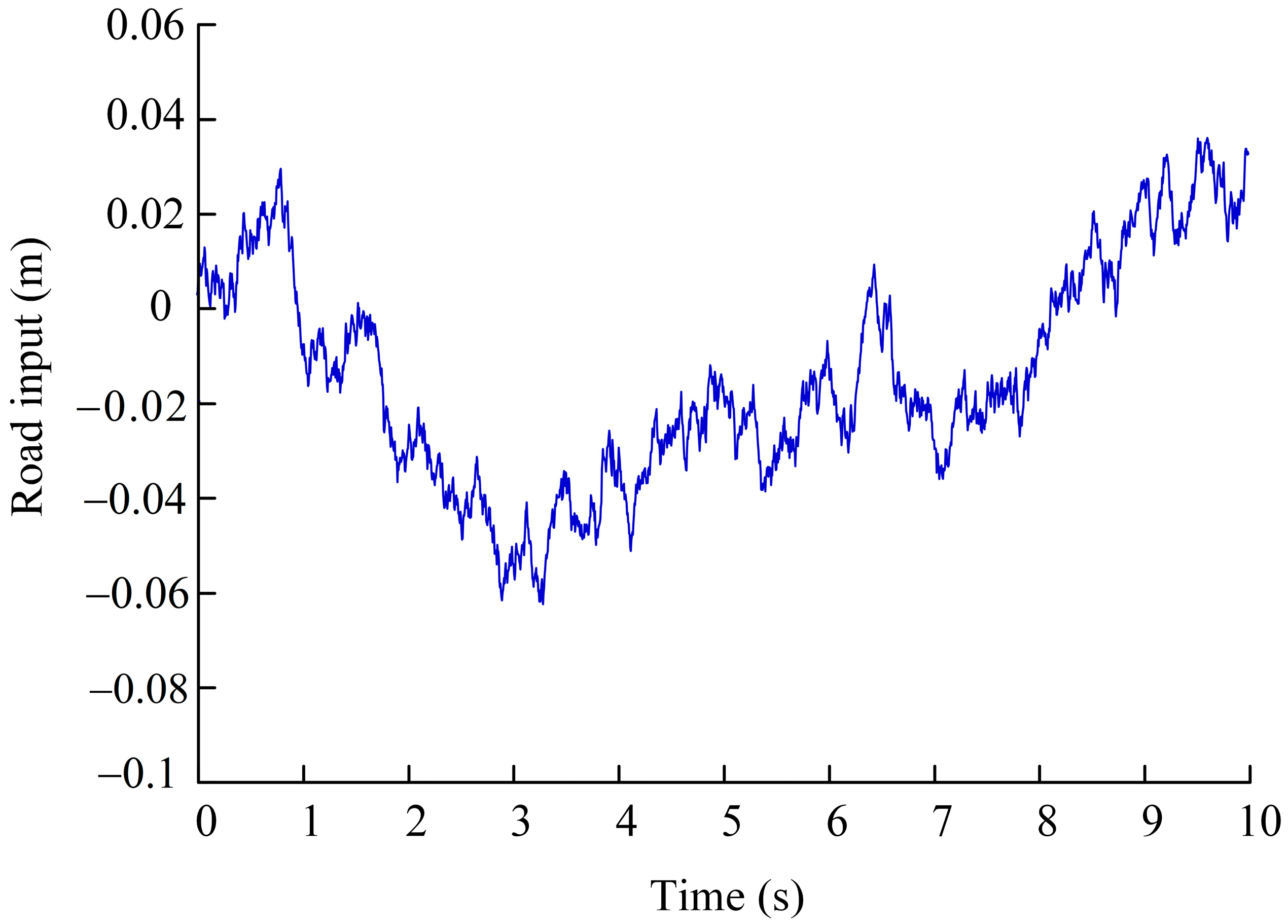
2.2. Road Excitation

The unevenness of the road surface is one of the main factors that has a key influence on the dynamic characteristics of suspension. When describing the pavement, it can be divided into two types: vibration excitation and impact excitation. Next, the road models of vibration excitation and impact excitation are constructed.

The vibration excitation comes from the continuous small unevenness of the road surface, and its frequency component has certain continuity and randomness. The fitting formula of the highway spectral density of the random road surface is as follows:

$$G_q(n)=G_q(n_0)({\displaystyle \frac{n}{n_0}}{)}^{-\omega }$$

(8)

where $n$ is the spatial frequency, $n=0.011~2.83 {\mathrm{m}}^{-1}$ $n_0$ is the reference spatial frequency, $n_0=0.1 {\mathrm{m}}^{-1}$; $G_q\left(n_0\right)$ is the road roughness coefficient. $\omega$ is the frequency index, so we take $\omega =2$.

By mathematical transformation and parametric processing of Equation (8), pavement time-domain excitation models with different vibration intensity levels can be constructed. The time-domain expression of random pavement is as follows:

$$\dot{q}(t)=-2\pi f_{0}q(t)+2\pi n_0\sqrt{G_q(n_0)v}\omega (t)$$

(9)

where $q(t)$ is road excitation; $f_0$ is the lower cutoff frequency; $\omega \left(t\right)$ is white noise.

Based on the random road excitation model defined in Equation (9), the Class C road condition was selected, the vehicle speed was set to 10 m/s, the lower cutoff frequency $f_0$ was set to 0.01 Hz, the noise intensity was set to 0.1 dB, the simulation time was set to 10 s, and the simulation step length was set to 0.01 s. The Class C road excitation generated under this condition is shown in Figure 2.

Shock excitation is usually caused by large bumps or potholes in the road surface, and its mathematical description often adopts a step function, pulse function, or sine function to simulate the actual bumps or potholes [23]. When the vehicle drives into the condition of the raised road surface with the height $h=0.11 \mathrm{m}$ and the length $l=0.6 \mathrm{m}$ at the time $1 \mathrm{s}<t<2 \mathrm{s}$ at the speed $v=10 \mathrm{m}/\mathrm{s}$, the sine wave signal is used as the input excitation. Figure 3 shows the time-domain signal of the raised road surface excitation.

$$x_r(t)=\left\{\begin{array}{cc}0& t>{\displaystyle \frac{l}{v}}\\ {\displaystyle \frac{h}{2}}\left[1-\mathit{cos}\left({\displaystyle \frac{2\pi v}{l}}t\right)\right]& 0\le t\le {\displaystyle \frac{l}{v}}\end{array}\right.$$

(10)

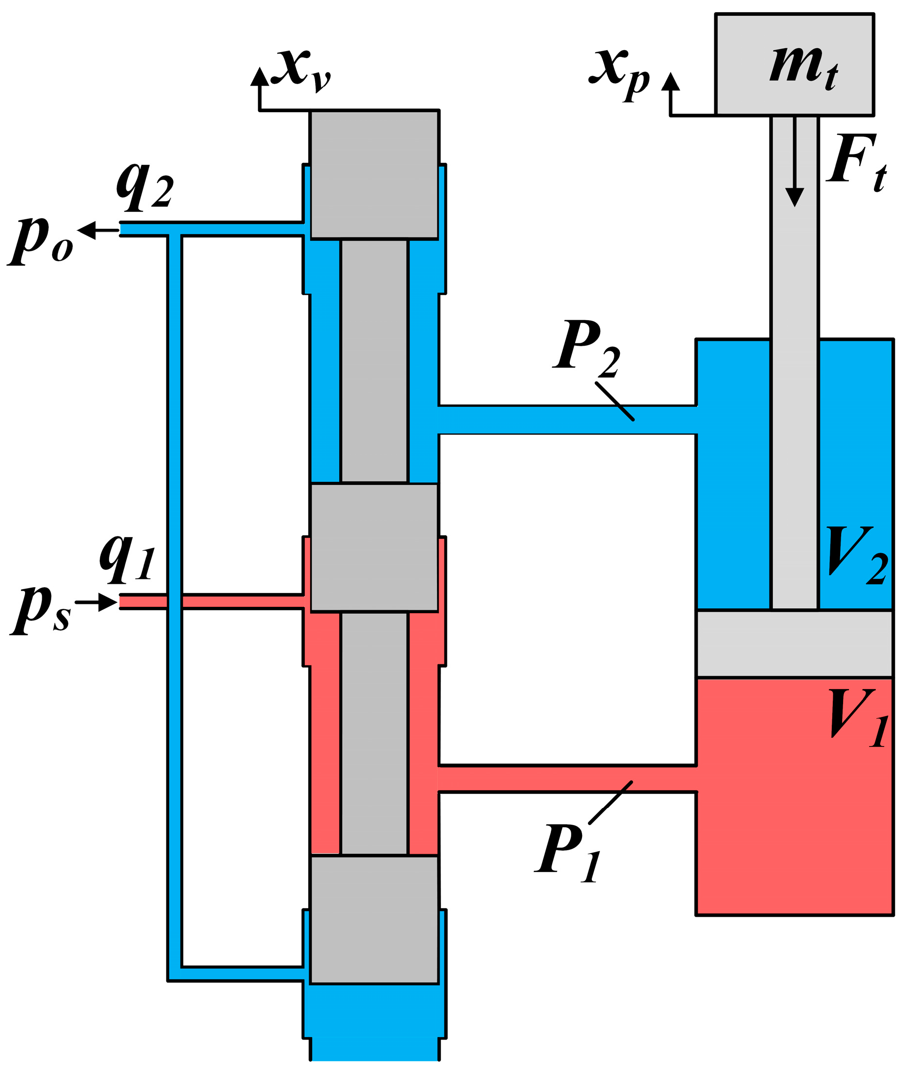
2.3. Modeling of Electro-Hydraulic Servo Actuator System

The structural form of an active suspension electro-hydraulic servo actuator is usually a electro-hydraulic servo valve control hydraulic cylinder, mainly including electro-hydraulic servo valve, hydraulic cylinder, load, and so on. In this paper, a valve-controlled asymmetrical hydraulic cylinder was selected as the structure of the electro-hydraulic servo actuator. The principle diagram of the active suspension electro-hydraulic servo actuator system is shown in Figure 4.

Aiming at the area difference of the rod cavity and the rodless cavity in the valve-controlled asymmetrical hydraulic cylinder, this section models and analyzes the two different flow gain conditions of piston rod extension and retract.

First, the modeling analysis in this section makes the following assumptions:

• It is assumed that the compressibility of the oil inside the servo valve is negligible.
• The oil supply pressure $p_s$ of the hydraulic system is constant, and the system oil return pressure $p_o$ is 0.
• The internal dynamic pressure loss of pipelines and valves is ignored.

(1)

The piston rod is extended.

When the piston rod is extended, that is, the spool displacement ($x_v>0$) and the spool moves upward, the rodless oil inlet flow $q_1$ and the rodded oil outlet flow $q_2$ of the hydraulic cylinder are, respectively,

$$q_1=C_{d}w{x}_v\sqrt{{\displaystyle \frac{2}{\rho }}(p_s-p_1)}$$

(11)

$$q_2=C_{d}w{x}_v\sqrt{{\displaystyle \frac{2}{\rho }}(p_2-p_o)}$$

(12)

where $x_v$—Servo valve spool displacement (m);

• $p_s$—System oil supply pressure (Pa);
• $p_o$—System oil return pressure (Pa);
• $C_d$—Servo valve port flow coefficient (m³/h);
• $w$—Servo valve port area gradient (m);
• $\rho$—System oil density (kg/m³).

The load flow $q_L$ and load pressure $p_L$ are defined as follows:

$$q_L={\displaystyle \frac{q_1+n{q}_2}{1+n^2}}$$

(13)

$$p_L=p_1-n{p}_2$$

(14)

where $p_1$—Hydraulic cylinder rodless chamber oil pressure (Pa);

• $p_2$—The hydraulic cylinder has the oil pressure of the rod cavity (Pa);
• $n$—Area ratio of the rod chamber to the rod-less chamber of the hydraulic cylinder ($n=A_2/A_1$).

It can be obtained by Equations (11)–(14):

$$p_1={\displaystyle \frac{p_L+n^3{p}_s}{1+n^3}}$$

(15)

$$p_2={\displaystyle \frac{n^2(p_s-p_L)}{1+n^3}}$$

(16)

Considering the leakage and compressibility of oil [24], the flow continuity equation of hydraulic cylinder can be expressed as follows:

$$q_1=A_1{\dot{x}}_p+{\displaystyle \frac{V_a+A_1{x}_p}{{\beta }_e}}{\dot{p}}_1+(C_b+C_a)p_1-C_b{p}_2$$

(17)

$$q_2=A_2{\dot{x}}_p+{\displaystyle \frac{V_b+A_2{x}_p}{{\beta }_e}}{\dot{p}}_2-(C_b+C_a)p_2+C_a{p}_1$$

(18)

where $x_p$—Displacement of the piston rod of hydraulic cylinder (m);

• ${\beta }_e$—Effective volumetric oil elastic modulus (Pa);
• $C_a$—Internal leakage coefficient of the hydraulic cylinder (Pa·m³/s);
• $C_b$—External leakage coefficient of hydraulic cylinder (Pa·m³/s);
• $A_1$, $A_2$—Effective area of the rodless cavity and the roded cavity (m²);
• $V_a$, $V_b$—Initial volume of rodless cavity and roded cavity of hydraulic cylinder (m³).

Valve spool moves upward:

$$q_L=A_1{\dot{x}}_p+{\displaystyle \frac{V_t}{4{\beta }_e}}{\dot{p}}_L+C_t{p}_L+C_1{p}_s$$

(19)

Among them, the total compression volume of hydraulic cylinder $V_t={\displaystyle \frac{4(V_a+n^3{V}_b)}{(1+n^3)(1+n^2)}}$, leakage coefficient $C_t={\displaystyle \frac{1+n}{1+n^3}}{C}_a+{\displaystyle \frac{C_b}{1+n^2}}$, $C_1={\displaystyle \frac{n^2(n^2-1)}{(1+n^2)(1+n^3)}}{C}_a$.

The hydraulic cylinder force balance equation is as follows:

$$A_1{P}_L=m_t{\ddot{x}}_p+B_p{\dot{x}}_p+F_t$$

(20)

where $m_t$—Equivalent load mass of the actuator (kg);

• $B_p$—Viscous damping coefficient of piston and load [N/(m/s)];
• $F_t$—Equivalent external load force of the actuator (N).

(2)

The piston rod retracts

The flow continuity equation of the rodless cavity and the roded cavity of the hydraulic cylinder is expressed as follows:

$$q_1=-A_1{\dot{x}}_p-{\displaystyle \frac{V_a+A_1{x}_p}{{\beta }_e}}{\dot{p}}_1-(C_a+C_b)p_1-C_a{p}_2$$

(21)

$$q_2=-A_2{\dot{x}}_p+{\displaystyle \frac{V_b+A_2{x}_p}{{\beta }_e}}{\dot{p}}_2+(C_a+C_b)p_2-C_a{p}_1$$

(22)

The valve core moves downward:

$$q_L=A_1{\dot{x}}_p+{\displaystyle \frac{V_t}{4{\beta }_e}}{\dot{p}}_L+C_t{p}_L+C_2{p}_s$$

(23)

$$\mathrm{where} C_2={\displaystyle \frac{n^2-1}{(1+n^2)(1+n^3)}}{C}_a$$

(24)

The hydraulic cylinder force balance equation is as follows:

$$A_1{P}_L=m_t{\ddot{x}}_p+B_p{\dot{x}}_p+F_t$$

(25)

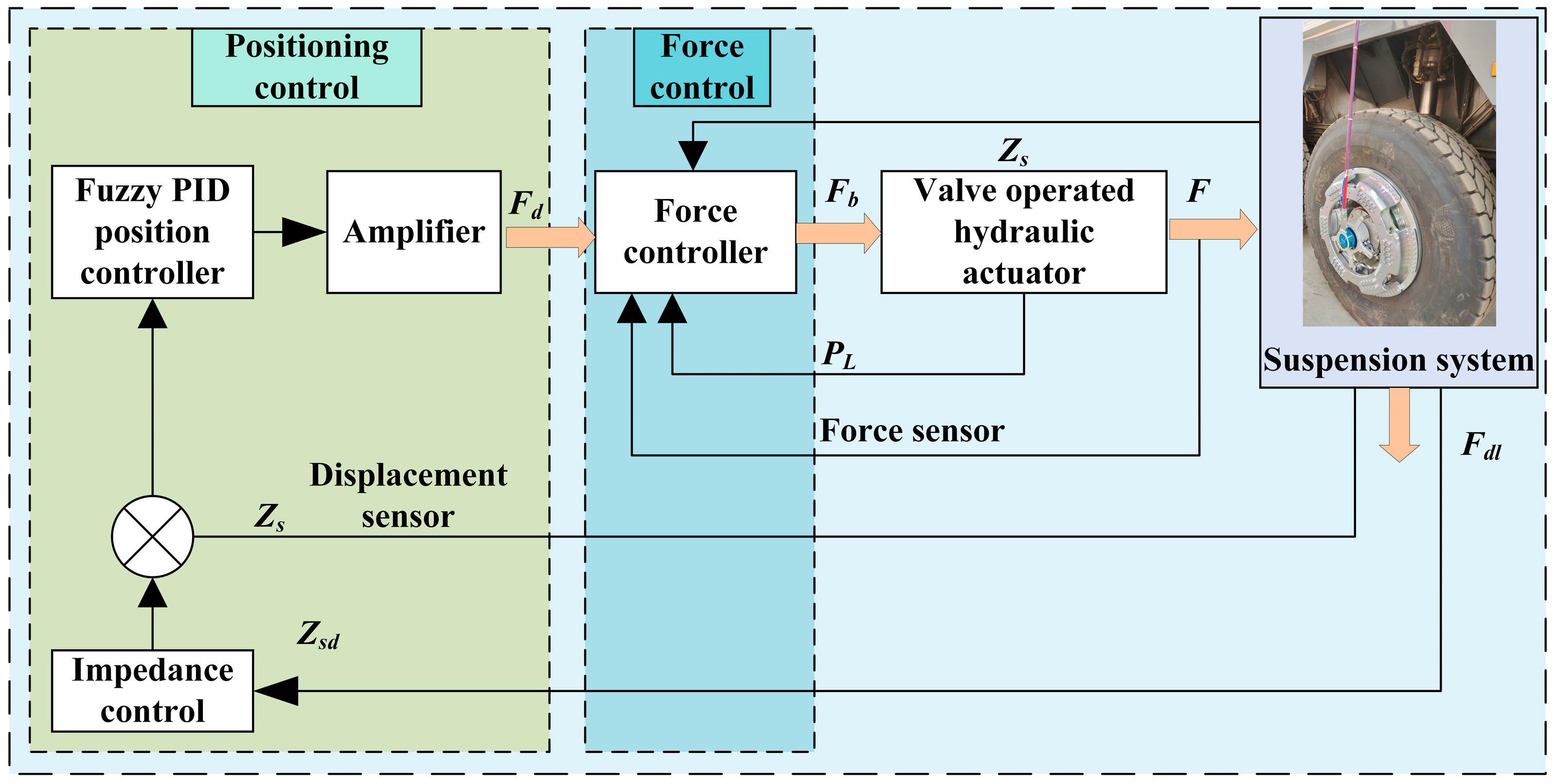
3. Optimal Control Based on Position and Force Feedback

In this section, the dynamic relationship of position tracking and force feedback is used to achieve the optimal control of suspension system. Figure 5 shows the structure of the active suspension control system, including a force controller, a position controller, and an impedance control for position tracking [25]. The system adopts a hydraulic servo actuator as the actuator. Although the hydraulic circuit has advantages such as high precision and large power to mass ratio [26], the hydraulic servo system can quickly respond to changes in input and output displacement and force, but due to the nonlinear characteristics of the hydraulic system and the correlation between the actuating force of the hydraulic cylinder and the vehicle body movement, the system error will inevitably increase.

Therefore, in order to improve the control accuracy of the system, this paper uses a linear feedback-constrained optimal control strategy to design the force controller. In the aspect of force tracking, the position controller is designed, and its output is set to the desired force of the hydraulic servo actuator. In order to achieve the goal of position tracking, the impedance control method is adopted to calculate the position correction amount of sprung mass according to the dynamic load of the wheel, and fuzzy PID position control is used to realize the fast tracking of the position correction amount of sprung mass. At the same time, combined with the spring-loaded mass displacement measured by the displacement sensor, these two parameters are used together as inputs to the position controller to ensure the coordinated operation between the various controllers of the system and realize the coordinated control of the entire system.

3.1. Force Control

The force control system adopts a double-loop structure; the inner loop control adopts linear feedback control, and the outer loop control adopts linear quadratic Gaussian (LQG) control. The LQG optimal controller generates the target control force, which is transmitted to the inner control ring as the input signal. The inner loop performs feedback control and feeds the control signal into the vehicle model. The real-time state variable of the vehicle is used as the output signal of the inner loop and fed back to the LQG controller. The structure of the force feedback optimal control system is shown in Figure 6.

(1)

Linear feedback

According to the analysis of the characteristics of the inner ring of the system, Formulas (20) and (25) can be obtained:

$$P_L={\displaystyle \frac{1}{A_1}}{F}_t+{\displaystyle \frac{1}{A_1}}{m}_t{\ddot{x}}_p+{\displaystyle \frac{1}{A_1}}{B}_p{\dot{x}}_p$$

(26)

$F_t$ is defined as control force and $F_d$ as desired control force. Linear feedback control is used to input the new control into ${\dot{F}}_t$ towards the desired force ${\dot{F}}_d$:

$${\dot{F}}_t-{\dot{F}}_d=k_p(F_d-F_t)$$

(27)

$$\dot{e}+k_p{e}_1=0$$

(28)

where $e_1=F_d-F_t$ is the error, and $k_p$ is the proportional coefficient. When time $t\to \infty$, the control force $F_t$ tends to the desired control force $F_d$.

By substituting Equation (27) into Equation (26), we obtain

$$P_L={\displaystyle \frac{1}{A_1(1+k_p)}}({\dot{F}}_d+k_p{F}_d)+{\displaystyle \frac{1}{A_1}}{m}_t{\ddot{x}}_p+{\displaystyle \frac{1}{A_1}}{B}_p{\dot{x}}_p$$

(29)

(2)

LQG control law

As mentioned in the above section, the suspension model state variables of the test sample vehicle in this project can be measured by sensors. A displacement sensor and a speedometer are installed in the center of the sprung mass and the unsprung mass, respectively, which can measure the position and speed of the two in real time. Selecting the active suspension system performance index function [27]:

$$J=\underset{T\to \infty }{lim}{\displaystyle \frac{1}{T}}E\left\{{\int }_0^T\left[q_1\right(z_s-z_u{)}^2+q_2(z_u-z_r{)}^2+q_3{\ddot{z}}_s^2+q_4{\ddot{z}}_u^2+r{U}^2]dt\right\}$$

(30)

where $q_1$—Weighting coefficient of suspension dynamic deflection;

• $q_2$—Wheel dynamic load weighting coefficient;
• $q_3$—Sprung mass acceleration weighting coefficient;
• $q_4$—Unsprung mass acceleration weighting coefficient;
• $r$—Active control force weighting coefficient.

Writing the above Equation (30) in matrix form, the following is obtained:

$$J=\underset{T\to \infty }{lim}{\displaystyle \frac{1}{T}}E\left({{\int }_0^T\left[\begin{array}{c}X\\ U\end{array}\right]}^{{\rm T}}\left[\begin{array}{cc}Q& M\\ M^T& R\end{array}\right]\left[\begin{array}{c}X\\ U\end{array}\right]dt\right)$$

(31)

where $Q$ is a semidefinite matrix, $Q=C_s^T\rho C_s$, $M=C_s^T\rho D_s$; $R$ is a positive definite matrix, $R=D_{\mathrm{s}}^{\mathrm{T}}\rho D_s+n$, where $\rho$ is the weighting matrix of state variables; $n$ is the control variable weighting matrix where $n=r$; $\rho =\mathrm{diag}\left[q_1{q}_2{q}_3{q}_4\right]$.

The optimal control force can be expressed as follows:

$$F_b=-KX$$

(32)

where $K=R^{-1}(B_s^{T}P+M^T)$.

The LQG control feedback gain matrix $K$ can be determined by solving the following Riccati Differential Equation:

$$P{A}_s+A_s^{T}P-M{R}^{-1}{B}_s^{T}P-M{R}^{-1}{M}^T-P{B}_s{R}^{-1}{B}_s^{T}P-P{B}_s{R}^{-1}{M}^T+Q=0$$

(33)

The feedback gain matrix k can be calculated by calling the LQR function in Matlab R2020a:

$$\left[\mathrm{KSE}\right]=\mathrm{LQR}(A_s,B_s,Q,R,M)$$

(34)

3.2. Position Control

The performance of a suspension system is primarily reflected in a vehicle’s ride comfort and handling stability, commonly measured by parameters such as body vibration displacement or acceleration. The goal of the one-sixth suspension structure discussed in this section is to physically reduce the vertical acceleration of the body as much as possible, while ensuring that the wheels have good ground contact and small dynamic loads.

In the system control architecture, the external loop position controller uses impedance control to generate position correction. Then, the fuzzy PID position controller adjusts the control force online in real time according to the position correction to realize the fast tracking of the body position correction.

(1)

Impedance control

Impedance control can combine position control and force control to realize dynamic coordination between the position and force of the controlled system. Based on the actual dynamic load of the wheel and predetermined impedance parameters, position correction is generated by the impedance control algorithm of the outer ring, and then, the dynamic characteristics of the suspension system defined by the impedance parameters are realized. The position impedance control model is described as follows:

$$F_{dl}=m_d{\ddot{z}}_{sd}+k_d{z}_{sd}+c_d{\dot{z}}_{sd}$$

(35)

where $m_d$—Ideal target inertia;

• $z_{sd}$—Expected displacement of the sprung mass;
• $k_d$—Ideal target stiffness;
• $c_d$—Ideal target damping.

According to above Equation (35), it can be seen that the ideal wheel dynamic load can be achieved by properly selecting the impedance control parameters, and the impedance control parameters can be reasonably selected according to the system requirements. Laplace transform processing of Equation (35) gives the following:

$$F_{dl}\left(s\right)=z_{sd}\left(s\right)(m_d{s}^2+k_d+c_{d}s)$$

(36)

where $F_{dl}\left(s\right)$ and $z_{sd}\left(s\right)$ are Laplace transforms of $F_{dl}$ and $z_{sd}$, respectively; $s^2{z}_{sd}\left(s\right)$ is the Laplace transform of the vertical acceleration of the sprung mass.

The transfer function model between the dynamic load of the wheel and the vertical acceleration of the body is established:

$$H(s)={\displaystyle \frac{F_{dl}(s)}{s^2{z}_{sd}(s)}}={\displaystyle \frac{m_d{s}^2+k_d+c_{d}s}{s^2}}$$

(37)

Frequency domain response is as follows:

$$\left|H(j\omega )\right|={\displaystyle \frac{1}{{\omega }^2}}{\left[(m_d{\omega }^2-k_d{)}^2+c_d^2{\omega }^2\right]}^{{\displaystyle \frac{1}{2}}}$$

(38)

Based on vehicle dynamics analysis, Equation (38) describes the relationship between vertical acceleration, wheel dynamic load, and impedance parameters, reflecting the internal correlation between vehicle ride comfort and handling stability.

From the perspective of the optimization of ride comfort, according to frequency domain analysis, in order to obtain good ride comfort, impedance parameters must meet the transfer function $\left|H\left(j\omega \right)\right|$ to maximize the amplitude–frequency response within the effective frequency band. Combined with the steady-state performance index and dynamic response characteristic analysis of the vibration model, the optimal boundary of the natural frequency ${\omega }_n$ of the target impedance model is ${\omega }_n=[{\displaystyle \frac{k_d}{m_d}}{]}^{{\displaystyle \frac{1}{2}}}$. When ${\omega }_n$ approaches zero, the sprung mass acceleration frequency $\omega$ will deviate from the characteristic frequency range of the system, so as to avoid the coupling resonance between sprung and unsprung.

In the control of wheel and ground force, in order to maintain a reasonable contact force between the wheel and ground, the damping coefficient $k_d$ should be minimized within the allowable range of system design to maintain the dynamic balance of tire–road contact. The damping coefficient $c_d$ is maximized to ensure the stability requirements of the dynamic response of the system during the transition process.

According to the frequency response characteristic analysis of Equation (38), when the excitation frequency $\omega \ne 0$ and $k_d<m_d{\omega }^2$ is satisfied, the transfer function $\left|H_1\left(j\omega \right)\right|$ will increase significantly when the mass parameter $m_d$ is increased. When $\omega =0$, $\left|H_1\left(j\omega \right)\right|=\infty$ for all $\forall F_{dyni}$. Therefore, through reasonable optimization and matching of the target impedance parameters $m_d$, $c_d$ and $k_d$, the vehicle ride comfort and handling stability can be effectively obtained.

(2)

Fuzzy PID position control

In the closed-loop control system, the PID controller detects the error signal between the output variable of the controlled system and the reference input in real time. The function expression of the deviation and the output signal is as follows:

$$e\left(t\right)=F_d\left(t\right)-c\left(t\right)$$

(39)

$$F(t)=K_{p}e(t)+K_i{\int }_0^{t}e(t)dt+K_d{\displaystyle \frac{de(t)}{dt}}$$

(40)

where $e(t)$ is the control deviation, which is the difference between the expected output $F_d\left(t\right)$ of the controlled object and the feedback value $c\left(t\right)$; $t$ is the time variable, which represents the dynamic process of the system; $F\left(t\right)$ is the output of the controller, that is, the adjustment action of the PID controller; $K_p$ is the proportional gain factor that determines the response strength of the system to the current deviation; $K_i$ is the integral gain coefficient used to eliminate steady-state error; $K_d$ is a differential gain coefficient used to suppress system overshoot and improve the dynamic response.

The core of fuzzy PID control is the dynamic optimization of PID control parameters by fuzzy rules. The body displacement error $e$ and its change rate $e_c$ are taken as input variables, and the output variables are the increment $△K_p$, $△K_i$ and $△K_d$ of PID control parameters. Its implementation process is as follows:

Fuzzification: The input variable and the membership function are mapped to the fuzzy set to complete the conversion from the exact value to the fuzzy value;

Fuzzy reasoning: Based on the preset fuzzy rule base, the input variables are logically judged through the reasoning mechanism to generate fuzzy output;

Defuzzification: The results of fuzzy inference are converted into precise PID parameter increment $△K_p$, $△K_i$, $△K_d$ by defuzzification algorithm;

Parameter adjustment: Real-time PID control parameters are updated according to the incremental value, that is,

$$\left\{\begin{array}{c}{K}_p=K_{p0}+△K_p\times q_p\hfill \\ K_i=K_{i0}+△K_i\times q_i\hfill \\ K_d=K_{d0}+△K_d\times q_d\hfill \end{array}\right.$$

(41)

Parameters in the formula: $K_{p0}$, $K_{i0}$, and $K_{d0}$ represent the initial tuning value of PID control, respectively; $q_p$, $q_i$, and $q_d$ are the correction coefficients of the fuzzy controller.

Control output: The optimized PID parameter is used to calculate the control force, and it is applied to the vehicle’s active suspension system to realize the rapid tracking adjustment of the body displacement correction.

In traditional PID control, the correction coefficient is usually a fixed value, resulting in the fact that the control parameters cannot be dynamically adjusted according to the real-time state of the system, and it is difficult to adapt to nonlinear changes under complex conditions, thus limiting its control performance in the whole test process [28]. On the other hand, although fuzzy control does not rely on accurate mathematical models but makes decisions based on an expert empirical rule base, its control accuracy is often limited by the completeness of the rule base and the accuracy of the reasoning mechanism, which may lead to steady-state errors [29]. In order to overcome the limitation of the above single control method, fuzzy PID control is adopted to improve the control performance significantly by combining the advantages of the two algorithms.

The fuzzy PID controller designed in this paper adopts a parameter autotuning mechanism, which can dynamically adjust the PID parameters according to the real-time state of the system, and its control principle is shown in Figure 7. The controller uses a fuzzy inference module to optimize PID parameters online, which not only retains the accuracy of PID control but also introduces the flexibility of fuzzy control, thus effectively improving the dynamic response characteristics and robustness of the system.

Both input and output variables of the controller are described using seven fuzzy subsets as linguistic variables, with their fuzzy sets defined as follows:

$$e,ec=\left\{NB,NM,NS,ZO,PS,PM,PB\right\}$$

(42)

Here, each element represents the following: NB (Negative Big), NM (Negative Medium), NS (Negative Small), ZO (Zero), PS (Positive Small), PM (Positive Medium), PB (Positive Big). The universe of discourse for all fuzzy variables is uniformly set to [−6, 6] to standardize input/output variables. Mamdani fuzzy inference [30] is adopted, which generates fuzzy outputs via ‘if-then’ rule-based max–min composition and obtains precise control quantity through defuzzification. The method assumes that the fuzzy rule base is complete and the reasoning mechanism is accurate, so as to ensure the control accuracy. At the same time, the input variables (vehicle displacement error e and its rate of change ec) are precisely fuzzy and defuzzy. Its limitation is that if the rule base is incomplete or the inference mechanism is biased, the control precision will be affected and the steady-state error may appear.

Based on expert knowledge and practical engineering experience, the design of the control rules follows the following principles:

(a)

When the vertical speed of the vehicle is opposite to the acceleration symbol, it indicates that the system has a tendency to cancel each other, and the control amount should be appropriately reduced to avoid excessive regulation.

(b)

When the vertical velocity and acceleration symbols are the same, it indicates that the system state presents a trend of continuous increase or decrease, and the control quantity should be appropriately increased to suppress its divergence trend. Because the Centroid Method can effectively smooth the system output and improve the precision of the defuzzification result, it is used to process the fuzzy output. The mathematical expression of the Centroid Method is as follows:

$$G^{*}={\displaystyle \frac{{\sum }_{i=1}^n{C}_i\cdot u\left(C_i\right)}{{\sum }_{i=1}^{n}u\left(C_i\right)}}$$

(43)

where $C_i$ is the $i$ element in the fuzzy output domain; $u\left(C_i\right)$ is the membership value corresponding to $C_i$; $n$ is the total number of output elements; $G^{*}$ is the exact output value after defuzzification.

Based on the dynamic characteristics and interaction of the proportional, integral and differential links in the control system, fuzzy rule sets for PID parameters self-tuning are designed, respectively. The fuzzy control rules of proportional gain increment $△K_p$, integral gain increment $△K_i$ and differential gain increment $△K_d$ are shown in

Table 1. $△K_p$ fuzzy control rules.

	∆kp	e
		NB	NM	NS	ZE	PS	PM	PB
	NB	PB	PB	PM	PM	PS	PS	ZE
	NM	PB	PM	PM	PM	PS	ZE	NS
	NS	PM	PM	PM	PS	ZE	NS	NS
ec	ZE	PM	PS	PS	ZE	NS	NM	NM
	PS	PS	PS	ZE	NS	NS	NM	NM
	PM	ZE	ZE	NS	NM	NM	NB	NB
	PB	ZE	NS	NS	NM	NM	NB	NB

,

Table 2. $△K_i$ fuzzy control rules.

	∆ki	e
		NB	NM	NS	ZE	PS	PM	PB
	NB	NB	NB	NM	NS	ZE	ZE	NB
	NB	NB	NM	NS	NS	ZE	ZE	NB
	NM	NM	NS	NS	ZE	PS	PS	NM
ec	NM	NS	NS	ZE	PS	PM	PM	NM
	NS	NS	ZE	PS	PM	PM	PM	NS
	ZE	ZE	PS	PM	PM	PB	PB	ZE
	ZE	ZE	PS	PM	PM	PB	PB	ZE

and

Table 3. $△K_d$ fuzzy control rules.

	∆kd	e
		NB	NM	NS	ZE	PS	PM	PB
	PS	PS	ZE	ZE	PS	PM	PB	PS
	NS	NS	NM	NS	ZE	NS	PM	NS
	NB	NM	NM	NS	ZE	PS	PM	NB
ec	NB	NM	NM	NS	ZE	PS	PM	NB
	NB	NM	NS	NS	ZE	PS	PS	NB
	NM	NS	NS	ZE	ZE	PS	PS	NM
	PS	ZE	ZE	PS	PM	PB	PB	PS

.

LQR [31]: LQR suspension controller parameters (q1–q6) were optimized by NSGA-II algorithm, and q1, q2, set q3 = q6 = 0.0007, S.T.0 ≤ q1 ≤ 10⁹, S.T.0 ≤ q2 ≤ 2800 were reasonably selected according to different working conditions.

In order to simplify the expression, the control algorithm is simplified as follows in the simulation: PS represents the passive suspension, LQR represents the constraint adaptive control, and FPL represents the fuzzy PID-LQG integrated control designed in this paper. In order to ensure the scientific comparison, the control algorithm comparison simulation analysis follows the following assumptions:

(1)

When the vehicle is driving on random road surface and raised road surface, the speed is 36 km/h, and the road surface is ISO-C grade road surface generated by the filtered white noise method. In the future, testing will be conducted at various speeds under C-class road condition.

(2)

The total travel constraint is set to ±110 mm. For the control strategy beyond the travel constraint, it is necessary to adjust the control parameters to keep them within the selected range.

(3)

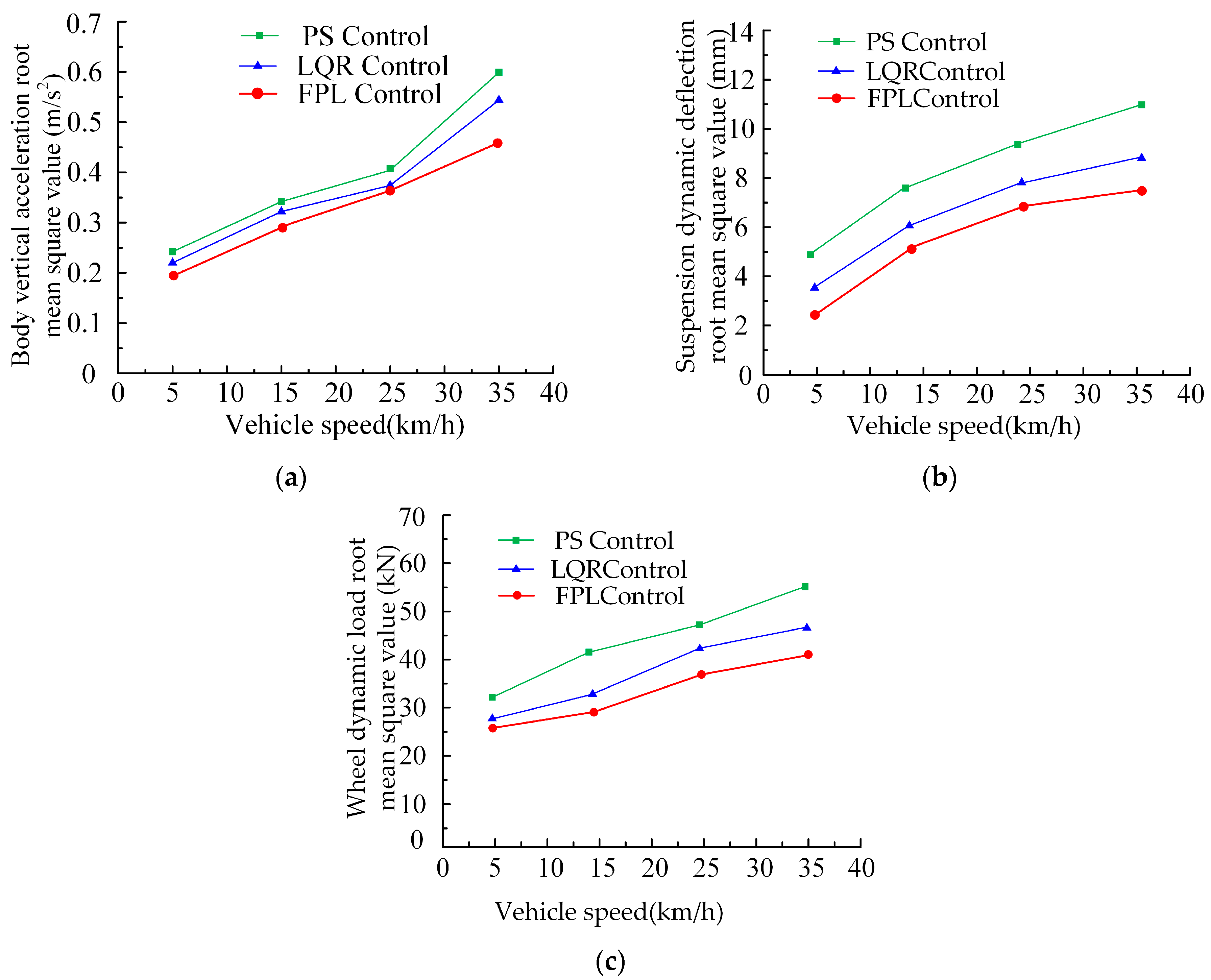
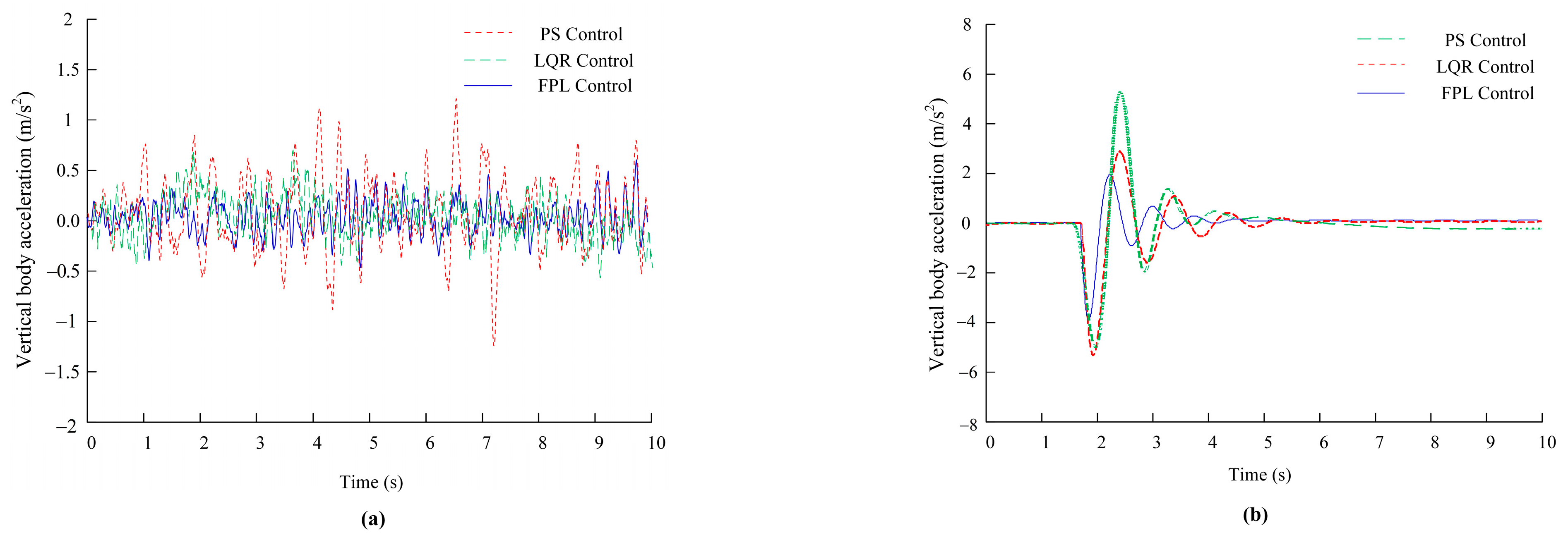
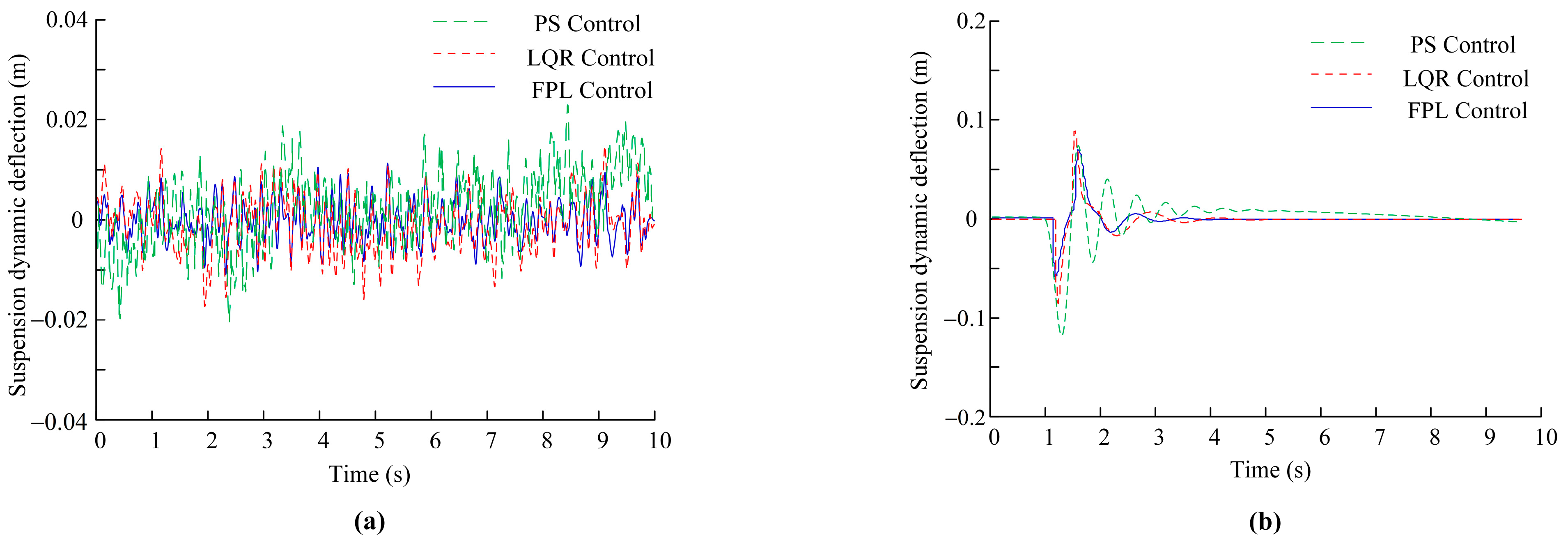
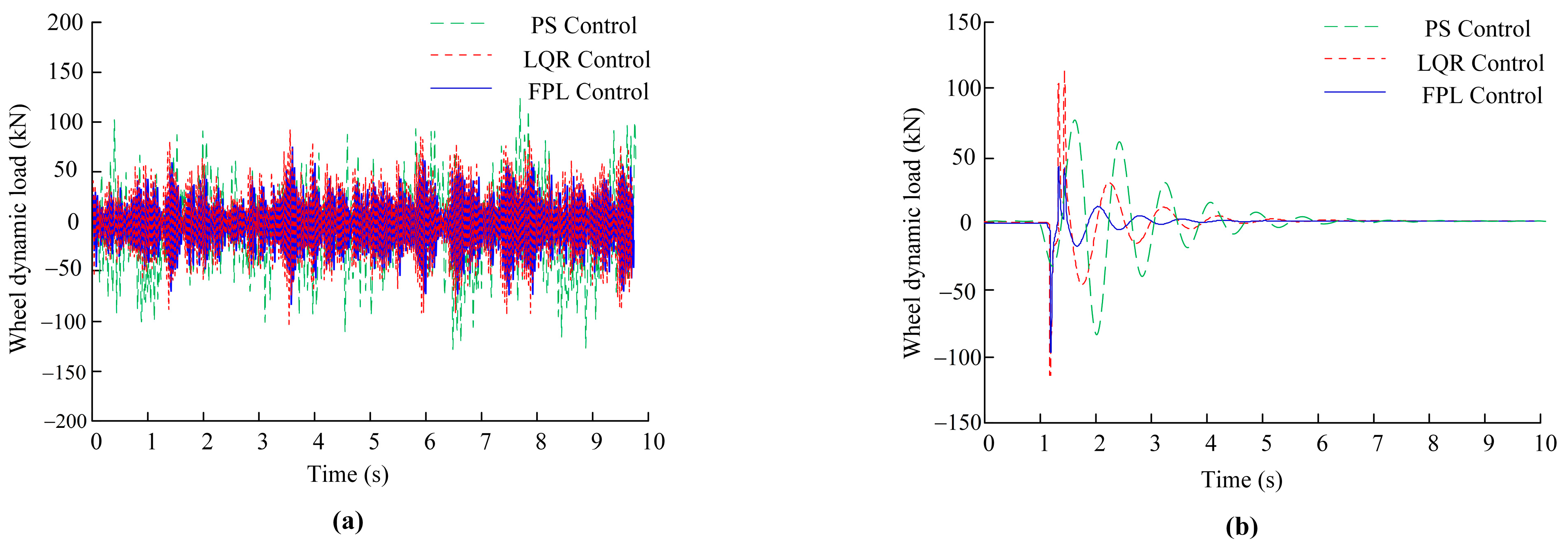
The passive suspension (PS), constraint adaptive control (LQR), and fuzzy PID-LQG (FPL) integrated control designed in this paper are not affected by system delay, and their performance is consistent with 0 ms delay in all cases.

4. Simulation Analysis

According to the designed active suspension position feedback and force feedback control actuators and their system dynamic characteristics analysis, the system simulation model was built under the Matlab R2020a/Simulink platform, and the suspension system simulation verification was carried out. The main simulation parameters of the system are summarized in

Table 4. Structural parameters of the active suspension system.

Parameters	Value
$\mathrm{Sprung} \mathrm{mass} m_s$/(kg)	5580
$\mathrm{Unsprung} \mathrm{mass} m_u$/(kg)	460
$\mathrm{Suspension} \mathrm{stiffness} k_s$/(kN·m−1)	5.8 × 106
$\mathrm{Suspension} \mathrm{damping} c_s$/(N·s·m−1)	8.7 × 103
$\mathrm{Tire} \mathrm{stiffness} k_t$/(kN·m−1)	1.96 × 106
$\mathrm{Tire} \mathrm{damping} c_t$/(N·s·m−1)	7.0 × 103
$\mathrm{Valve} \mathrm{port} \mathrm{flow} \mathrm{coefficient} C_d$	0.7
$\mathrm{System} \mathrm{oil} \mathrm{density} \rho$/(kg·m−3)	860
$\mathrm{Effective} \mathrm{volumetric} \mathrm{oil} \mathrm{elastic} \mathrm{modulus} {\beta }_e$/(Pa)	7.0 × 108
$\mathrm{Effective} \mathrm{area} \mathrm{of} \mathrm{rod}-\mathrm{free} \mathrm{cavity} A_1$/(m2)	5.67 × 10−3
$\mathrm{Effective} \mathrm{area} \mathrm{of} \mathrm{rod} \mathrm{cavity} A_2$/(m2)	1.26 × 10−3
$\mathrm{System} \mathrm{oil} \mathrm{supply} \mathrm{pressure} p_s$/(Pa)	2.5 × 107

. The excitation input of C-class road condition (Figure 2) and 0.11 m raised road condition (Figure 3) was, respectively, selected into the passive suspension model and the position–force feedback controlled active suspension model system. Figure 8, Figure 9 and Figure 10 shows that under the excitation of C-class road condition and raised road condition, the time-domain variation contrast curves of vertical acceleration, dynamic deflection of suspension and dynamic load of wheel of vehicle passive suspension and active suspension, and the root-mean-square values of each evaluation index of suspension are shown in

Table 5. Comparison of root-mean-square values of suspension evaluation indicators.

Working Conditions	Control Mode	Vehicle Vertical Acceleration/(m·s−2)	Suspension Dynamic Deflection/m	Dynamic Wheel Load/kN
Class C road	PS Control	0.5273	0.009932	49.2491
	LQR Control FPL Control	0.4125 0.3028	0.006751 0.004158	37.2455 33.8156
Decline ratio/%	LQR versus PS FPL versus PS	21.77% 42.58%	32.03% 58.14%	24.37% 31.34%
Raised road	PS Control	1.3542	0.02191	48.4185
	LQR Control	0.8924	0.01352	36.5326
	FPL Control	0.6512	0.00904	23.6748
Decline ratio/%	LQR versus PS FPL versus PS	34.10% 51.91%	38.29% 58.74%	24.55% 51.1%

.

Taking the C-class road as an example, the FPL control strategy proposed in this paper is compared with the LQR control and PS control strategies. When the vehicle speed is about 5 km/h, 15 km/h, 25 km/h, and 35 km/h, respectively, the root-mean-square values of the body vertical acceleration, suspension dynamic deflection, and wheel dynamic load are compared, as shown in Figure 8.

It can be clearly seen from Figure 8 that when the vehicle speed is about 5 km/h, 15 km/h, 25 km/h and 35 km/h, compared with PS control and LQR control, under the FPL control strategy, the vertical acceleration of the body, the dynamic deflection of the suspension and the root-mean-square value of the dynamic load of the wheel all decrease to different degrees. And the higher the speed, the greater is the reduction trend. This fully indicates that the FPL integrated control scheme designed in this paper can effectively improve the ride comfort and handling stability of vehicles, especially when the speed is fast, this improvement effect is more significant. When the root-mean-square value of the vehicle speed is about 36 km/h, the specific results of the vehicle passing through the C-class road surface and the raised road surface are shown in Figure 9, Figure 10 and Figure 11.

As shown in Figure 9, Figure 10 and Figure 11, compared with passive PS control and LQR adaptive control, FPL integrated control strategy was adopted for active suspension in this study, and the peak value of vertical acceleration of the body, the peak value of dynamic deflection of the suspension and the peak value of dynamic load of the wheel were significantly reduced when facing the excitation condition of C-class road surface and 0.11 m raised road surface. At the same time, the active suspension controller exhibited faster output response and better real-time performance. Especially under the excitation of 0.11 m raised road surface, the oscillation times of the waveform were greatly reduced and quickly became a stable state.

Further observation of Figure 9, Figure 10 and Figure 11 and data from Table 5 show that under the excitation condition of C-class road surface, the root-mean-square values of body vertical acceleration, suspension dynamic deflection, and wheel dynamic load under the integrated control of LQR adaptive control and FPL designed in this paper decrease by 21.77% 32.03%, 24.37%, and 42.58%, 58.14%, 31.34%, respectively, compared with the passive PS control. In the case of 0.11 m road excitation, the root-mean-square values of these three indexes of FPL integrated control decreased more significantly, reaching 51.91%, 58.74% and 51.1%, respectively, which met the design requirements of this paper to reduce the vibration of the car body, reduce the dynamic load of the wheel and ensure that the wheel has good grounding ability.

This control strategy is not only suitable for the vibration excitation scenario of C-class road with various speeds and fixed speed, but also has good applicability for the impact excitation condition of a raised road. It can be seen that the control method proposed in this study can effectively improve the performance of the suspension system, significantly enhance the ride comfort of the vehicle, and significantly improve the handling stability of the vehicle.

5. Conclusions

Based on the constructed model, this paper selects body vertical acceleration, suspension dynamic deflection, and wheel dynamic load as key performance indicators to evaluate the control effect and draws the following conclusions:

(1)

Based on fully considering the nonlinear mechanical characteristics of the hydraulic actuator, a one-sixth vehicle structure model and a valve-controlled hydraulic actuator system model are constructed. A multi-closed-loop control strategy for position–force feedback optimal control of a valve-controlled hydraulic active suspension system is further proposed. A fuzzy PID position controller and a linear feedback-LQG optimal force controller are designed, and an impedance control is designed to track the dynamic load of the wheel to achieve accurate correction of the sprung mass position.

(2)

With the help of the theoretical analysis and simulation test of the control algorithm, the vehicle is subjected to the working condition test of the excitation input of C-class road surface and raised road surface at varying speeds and fixed speeds. The results strongly confirm that the active suspension with fuzzy PID position and linear feedback LQG optimal force control algorithm is better than the passive PS control and LQR adaptive control, achieving control optimization goals more efficiently. Under different road conditions and various speed incentives, the relevant performance indexes show a significant downward trend. The results show that the designed controller can reduce the vibration transmission of the vehicle during driving, reduce the impact on the suspension system, improve the grounding ability of the wheel, and improve the ride comfort and handling stability of the vehicle. The controller shows good road adaptability both on the C-class road surface and the raised road surface, which further verifies the effectiveness of the proposed control strategy in improving vehicle passability.

References

1. Shah, D.; Santos, M.M.D.; Chaoui, H.; Justo, J.F. Event-Triggered Non-Switching Networked Sliding Mode Control for Active Suspension System With Random Actuation Network Delay. IEEE Trans. Intell. Transp. Syst. 2022, 23, 7521–7534. [Google Scholar] [CrossRef]
2. Rath, J.J.; Defoort, M.; Sentouh, C.; Karimi, H.R.; Veluvolu, K.C. Output-Constrained Robust Sliding Mode Based Nonlinear Active Suspension Control. IEEE Trans. Ind. Electron. 2020, 67, 10652–10662. [Google Scholar] [CrossRef]
3. Wang, J.J.; Zhao, J.Y.; Cai, W.; Li, W.L.; Jia, X.; Wei, P. Leveling Control of Vehicle Load-Bearing Platform Based on Multisensor Fusion. J. Sens. 2021, 2021, 7. [Google Scholar] [CrossRef]
4. Chen, H.; Liu, Y.J.; Liu, L.; Tong, S.C.; Gao, Z.W. Anti-Saturation-Based Adaptive Sliding-Mode Control for Active Suspension Systems With Time-Varying Vertical Displacement and Speed Constraints. IEEE Trans. Cybern. 2022, 52, 6244–6254. [Google Scholar] [CrossRef]
5. Liu, H.; Li, S.H.; Zhang, P.Q. Rigid flexible coupling speclal vehicle dynamic analysis and suspension optimization of obstracle crossing. J. Dyn. Control 2021, 19, 74–82. [Google Scholar]
6. Zhang, X.D.; Göhlich, D.; Zheng, W. Karush-Kuhn-Tuckert based global optimization algorithm design for solving stability torque allocation of distributed drive electric vehicles. J. Frankl. Inst.-Eng. Appl. Math 2017, 354, 8134–8155. [Google Scholar] [CrossRef]
7. Yang, T.; Sun, J.; Liu, Z.; Wang, J. Research on Suspension Systems Control for Heavy Duty Transport Vehicles under Extreme Operating Conditions Considering Handling Stability. J. Transp. Res. Board 2025, 03611981251315691. [Google Scholar] [CrossRef]
8. Xiong, X.; Pan, Z.; Liu, Y.; Yue, J.; Xu, F. An adaptive backstepping sliding mode control strategy for the magnetorheological semi-active suspension. J. Automob. Eng. 2024, 09544070241260454. [Google Scholar] [CrossRef]
9. Ji, G.; Li, S.; Feng, G.; Li, Z.; Shen, X. Time-delay compensation control and stability analysis of vehicle semi-active suspension systems. Mech. Syst. Signal Process. 2025, 228, 112414. [Google Scholar] [CrossRef]
10. Xing, X.Y.; Burdet, E.; Si, W.Y.; Yang, C.G.; Li, Y.A. Impedance Learning for Human-Guided Robots in Contact With Unknown Environments. IEEE Trans. Robot. 2023, 39, 3705–3721. [Google Scholar] [CrossRef]
11. Sharifi, M.; Azimi, V.; Mushahwar, V.K.; Tavakoli, M. Impedance Learning-Based Adaptive Control for Human-Robot Interaction. IEEE Trans. Control Syst. Technol. 2022, 30, 1345–1358. [Google Scholar] [CrossRef]
12. An, H.; Ye, C.; Yin, Z.; Lin, W. Neural Adaptive Impedance Control for Force Tracking in Uncertain Environment. Electronics 2023, 12, 640. [Google Scholar] [CrossRef]
13. Ulkir, O.; Akgun, G.; Kaplanoğlu, E.J.S.i.I. Real-Time Implementation of Data-Driven Predictive Controller for an Artificial Muscle. Stud. Inform. Control 2019, 28, 189–200. [Google Scholar] [CrossRef]
14. Flayyih, M.A.; Hamzah, M.N.; Hassan, J.M. Nonstandard Backstepping Based Integral Sliding Mode Control of Hydraulically Actuated Active Suspension System. Int. J. Automot. Technol. 2023, 24, 1665–1673. [Google Scholar] [CrossRef]
15. Nazemian, H.; Masih-Tehrani, M. Development of an optimized game controller for energy saving in a novel interconnected air suspension system. Proc. Inst. Mech. Eng. Part D-J. Automob. Eng. 2020, 234, 3068–3080. [Google Scholar] [CrossRef]
16. Guo, S.J.; Chen, L.; Wang, X.K.; Zou, J.Y.; Hu, S.B. Hydraulic Integrated Interconnected Regenerative Suspension: Modeling and Characteristics Analysis. Micromachines 2021, 12, 22. [Google Scholar] [CrossRef]
17. Ding, F.; Liu, J.; Jiang, C.; Du, H.P.; Zhou, J.X.; Lei, F. Vibration suppression investigation and parametric design of tri-axle straight heavy truck with pitch-resistant hydraulically interconnected suspension. J. Vib. Control 2022, 28, 3823–3840. [Google Scholar] [CrossRef]
18. Fu, Y.M.; Zhou, X.J.; Wan, B.W.; Yang, X.F. Decoupled adaptive terminal sliding mode control strategy for a 6-DOF electro-hydraulic suspension test rig with RBF coupling force compensator. Proc. Inst. Mech. Eng. Part C-J. Eng. Mech. Eng. Sci. 2023, 237, 4339–4357. [Google Scholar] [CrossRef]
19. Ozbek, C.; Ozguney, O.C.; Burkan, R.; Yagiz, N. Ride comfort improvement using robust multi-input multi-output fuzzy logic dynamic compensator. Proc. Inst. Mech. Eng. Part I-J. Syst. Control Eng. 2023, 237, 72–85. [Google Scholar] [CrossRef]
20. Bashir, A.O.; Rui, X.T.; Abbas, L.K.; Zhang, J.S. Ride Comfort Enhancement of Semi-active Vehicle Suspension Based on SMC with PID Sliding Surface Parameters Tuning using PSO. Control Eng. Appl. Inform. 2019, 21, 51–62. [Google Scholar]
21. Fu, B.; Liu, B.B.; Di Gialleonardo, E.; Bruni, S. Semi-active control of primary suspensions to improve ride quality in a high-speed railway vehicle. Veh. Syst. Dyn. 2023, 61, 2664–2688. [Google Scholar] [CrossRef]
22. Saglam, F.; Unlusoy, Y.S. Adaptive ride comfort and attitude control of vehicles equipped with active hydro-pneumatic suspension. International J. Veh. Des. 2016, 71, 31–51. [Google Scholar] [CrossRef]
23. Wang, Y.Y.; Li, P.F.; Ren, G.Z. Electric vehicles with in-wheel switched reluctance motors: Coupling effects between road excitation and the unbalanced radial force. J. Sound Vib. 2016, 372, 69–81. [Google Scholar] [CrossRef]
24. Xu, Z.Q.; Li, W.L.; Liu, X.Y.; Chen, Z.X. Dynamic characteristics of coupling model of valve-controlled cylinder parallel accumulator. Mech. Ind. 2019, 20, 18. [Google Scholar] [CrossRef]
25. Fateh, M.M.; Alavi, S.S. Impedance control of an active suspension system. Mechatronics 2009, 19, 134–140. [Google Scholar] [CrossRef]
26. Wang, G.; Chadli, M.; Basin, M.V. Practical Terminal Sliding Mode Control of Nonlinear Uncertain Active Suspension Systems With Adaptive Disturbance Observer. IEEE-ASME Trans. Mechatron. 2021, 26, 789–797. [Google Scholar] [CrossRef]
27. Zhao, W.P.; Gu, L. Hybrid Particle Swarm Optimization Genetic LQR Controller for Active Suspension. Appl. Sci. 2023, 13, 14. [Google Scholar] [CrossRef]
28. Sathishkumar, P.; Jancirani, J.; John, D.; Arun, B. Controller Design for Convoluted Air spring system controlled Suspension. Appl. Mech. Mater. 2014, 592–594, 1025–1029. [Google Scholar] [CrossRef]
29. Huang, Y.B.; Wu, X.; Na, J.; Gao, G.B.; Guo, Y. Active Suspension Control for Vehicle Systems with Prescribed Performance. J. Vib. Eng. Technol. 2017, 5, 407–416. [Google Scholar]
30. Najafi, A.; Masih-Tehrani, M.; Emami, A.; Esfahanian, M. A modern multidimensional fuzzy sliding mode controller for a series active variable geometry suspension. J. Braz. Soc. Mech. Sci. Eng. 2022, 44, 23. [Google Scholar] [CrossRef]
31. Lu, Y.; Zhen, R.; Liu, Y.; Zhong, J.; Sun, C.; Huang, Y.; Khajepour, A. Practical solution for attenuating industrial heavy vehicle vibration: A new gain-adaptive coordinated suspension control system. Control Eng. Pract. 2025, 154, 106125. [Google Scholar] [CrossRef]
Figure 1. Schematic diagram of the one-sixth suspension system: (a) passive suspension model, (b) active suspension model.
Processes 13 01241 g001
Figure 2. Class C road excitation.
Processes 13 01241 g002
Figure 3. Raised road surface excitation.
Processes 13 01241 g003
Figure 4. Structure diagram of valve-controlled asymmetric hydraulic cylinder.
Processes 13 01241 g004
Figure 5. Cooperative control structure of active suspension system.
Processes 13 01241 g005
Figure 6. Optimal control structure of force feedback.
Processes 13 01241 g006
Figure 7. Fuzzy PID control principle.
Processes 13 01241 g007
Figure 8. (a). Comparison of RMS values of vertical acceleration of vehicle body. (b). Comparison of root-mean-square values of suspension dynamic deflection. (c). Comparison of root-mean-square values of wheel dynamic load.
Processes 13 01241 g008
Figure 9. Comparison of body vertical acceleration between C-class road (a) and raised road (b).
Processes 13 01241 g009
Figure 10. Comparison of suspension dynamic deflection between C-class road (a) and raised road (b).
Processes 13 01241 g010
Figure 11. Comparison of wheel dynamic load between C-class road (a) and raised road (b).
Processes 13 01241 g011