Bearing Fault Diagnosis Based on Multiscale Lightweight Convolutional Neural Network

Abstract

Many bearing fault diagnosis methods often struggle to balance between adequate feature extraction and lightweight property, which makes it somewhat difficult to fulfill the accuracy and efficiency required for practical applications. To address this issue, this study describes the development of a multiscale lightweight deep learning model for accurate bearing fault diagnosis. Specifically, the Gaussian pyramid method, which can create a series of images at different scales, is employed to express the Gramian angular field (GAF) matrix images generated by transforming the bearing vibration signals to avoid the common problem of insufficient feature extraction of a single-scale image. At the same time, the dependencies between feature channels are extracted using a lightweight attention mechanism utilized in deep learning, known as Efficient Channel Attention (ECA), to improve the capability of feature representation. This approach effectively improves the learning ability of bearing fault characteristics and greatly increases the accuracy of fault diagnosis. Considering the problem related to the lightweight level of the method, a Ghost module, a type of convolution neural network system, is also employed to generate more features by using fewer parameters, thereby improving the overall calculation efficiency. Here we have developed a residual module based on the Ghost module and ECA, which can be easily integrated into most bearing fault diagnosis backbone networks. Based on our experimental tests, the developed system can clearly achieve high accuracy precision of bearing fault diagnosis to fulfill the needs of practical engineering while maintaining light weight. Specifically, the test accuracy of the proposed method using two bearing fault datasets exceeds 99.4%, and the giga floating-point operations (GFLOPs) is only 1.99, which can fully meet the needs of practical engineering.

1. Introduction

Bearing is a key component in rotating machinery, and its constant operation directly affects the stability and safety of the entire mechanical system. Bearing faults are often caused by chemical and physical deterioration including wear, fatigue, corrosion, and more. Early detection and timely handling of bearing faults are essential to ensure the normal operation and maintenance of equipment and to prevent unscheduled downtime. Existing bearing fault diagnosis methods are often classified into three categories according to the different feature extraction methods: traditional signal processing methods [1], machine learning methods [2], and deep learning methods [3,4].

Bearing fault diagnosis based on traditional signal processing methods extracts relevant features of measurement signals from various perspectives and determines the health status of the bearing through feature analysis. The types of features extracted from signals mainly include time-domain features, frequency-domain features, time–frequency-domain comprehensive features, as well as signal distribution features such as information entropy and fractals [5,6,7,8]. Complete ensemble empirical modal decomposition with adaptive noise was also used to extract time-domain features while performing two fast Fourier transforms for deep frequency-domain feature extraction [9]. In addition, the recursive feature elimination combined with the chi-square test was utilized to select the optimal feature subset from the obtained time–frequency features [10]. Based on these optimal features, various classifiers have been developed for bearing fault diagnosis. Upon collecting the signals from rolling bearings by vibration sensors, the mean square value served as an indicator to accurately extract early fault signals [11]. A combined method has also been presented using multiscale weighted entropy morphological filtering signal processing and bidirectional long- and short-term memory neural networks [12]. A nonlinear symplectic entropy measure analysis method was presented to analyze the measured signals for fault monitoring of rolling bearings [13].

Machine learning models including Support Vector Machine (SVM) and K-Nearest Neighbors (KNN) are used to diagnose bearing faults [2,14]. This powerful learning method effectively reduced the dependence on expert knowledge, which required effective integration of feature vectors, often resulting in higher diagnostic accuracy than human judgment and a more adaptive and higher level of automation than traditional methods. For example, using SVM to predict the generator output power of wind turbines, the residual difference between the actual generator output power and the predicted output power was calculated, which directly reflected the operating state and fault development trend of the fan main bearing through the changing trend of the residual difference [14,15,16]. Non-stationary bearing vibration signals were decomposed using double-tree wavelet packet transform, and the extracted energy features of each frequency band were input to SVM for bearing fault diagnosis [17]. Variational modal decomposition was combined with SVM to achieve good results in rolling bearing fault diagnosis experiments [18,19,20]. After performing wavelet packet decomposition of bearing vibration signals, energy coefficients of signals in each frequency band were extracted, where the features selected by the Fisher ratio method were input into SVM to realize bearing fault diagnosis with a small number of samples [21]. Using empirical modal decomposition (EMD) to decompose the vibration signal into several eigenmodal components, an autoregressive model was established for each component to calculate the residuals using SVM for rolling bearing fault diagnosis [22,23]. It is noted that these methods maintain a high fault diagnosis accuracy for a small number of samples.

The bearing fault diagnosis method based on deep learning can simultaneously extract fault features and identify faults in a holistic and adaptive way [3,4,24]. Therefore, there is less reliance on expert knowledge, a higher level of automation, and stronger learning ability, which can achieve end-to-end bearing fault diagnosis. A bearing fault diagnosis method that combines hybrid feature pooling and deep neural network (DNN) based on sparse automatic encoder (SAE) to effectively diagnose multiple bearing fault types with the degree of fault severities simultaneously [25]. An attention-intensive convolutional neural network was used by combining dense convolutional blocks with an attention mechanism to verify the effectiveness of the model in rolling bearing fault diagnosis through different datasets [26,27]. Since time-domain vibration signals are time-series data with high sampling frequency, recurrent neural networks can also be applied to bearing fault diagnosis, among which long short-term memory (LSTM) is more commonly utilized. For example, the features with high temperature correlation of gearbox bearings were extracted through the general mutual information method to build an LSTM neural network deep learning model that predicted the temperature of gearbox bearings of wind motors, thereby realizing the fault diagnosis of fan bearings [28,29,30]. Another deep learning method was reported by combining an end-to-end convolutional neural network and LSTM [31]. This method used the equal-long time series data collected by sensors as input and achieved the highest bearing fault detection accuracy in the shortest possible time without complicated data signal preprocessing. In addition, in order to improve the feature extraction ability and lightweight level of deep learning models, some attention mechanisms and lightweight methods have been proposed [32,33]. These methods can be used to improve the performance of fault diagnosis models. As shown in

Table 1. Comparison of bearing fault diagnosis methods.

Methodology	Representative Works	Advantages	Disadvantages
Traditional signal processing methods	Time-domain features, frequency-domain features, time–frequency-domain features, and signal distribution features [5,6,7,8]. Two FFT (fast Fourier transforms) deep frequency domain analyses [9]. The recursive feature elimination combined with the chi-square test [10]. Mean square value indicator [11]. Multiscale weighted entropy morphological filtering [12]. Nonlinear symplectic entropy measure analysis [13].	Strong multidimensional feature extraction capability and wide adaptability. Effectively deal with non-smooth signals.	Relying on expert experience to design features. High computational complexity. Generalization ability for small samples and complex failure modes is limited.
Machine learning methods	SVM combined with residual analysis to predict fan bearing status [14,15,16]. Double-tree wavelet packet transform, SVM [17]. Variational modal decomposition, SVM [18,19,20]. Wavelet packet decomposition, SVM [21]. EMD, Autoregressive model, SVM [22,23].	Reduction of dependence on expert knowledge. A higher degree of automation. High diagnosis accuracy is maintained with small samples.	Features need to be artificially designed. Weak model interpretability. Limited ability to process high-dimensional data.
Deep learning methods	Combining hybrid feature pooling with DNN based on SAE [25]. Attention-intensive convolutional neural network [26,27]. LSTM temperature prediction model [28,29,30]. Combining end-to-end convolutional neural network and LSTM [31]. Attention mechanisms, lightweight methods [32,33].	End-to-end automatic feature extraction. Strong nonlinear modeling capability. Adaptation to complex working conditions. High diagnostic efficiency.	Reliance on massively labeled data. High consumption of computational resources. Poor model interpretability.

, various bearing fault diagnosis methods are summarized into three main categories.

Lately, significant research progress has been made in bearing fault diagnosis, but there are still some problems that need to be solved: (1) Given the complex types and causes of bearing defects, it is difficult to extract key features at a single scale, leading to low accuracy in fault diagnosis. Therefore, it is necessary to enhance the capability of multiscale feature extraction by improving the network framework, and at the same time, to study the main mechanism to advance the adequacy of key feature expression. (2) Deep learning network models are complex and difficult to apply to practical engineering applications. Thus, it is urgent to study the lightweight convolutional mode to improve the lightweight level of the network.

To overcome these problematic issues, this work demonstrates the utilization of a multiscale lightweight deep learning model to diagnose bearing faults accurately and simultaneously. First, the Gaussian pyramid method is used to represent the Gramian angular field (GAF) matrix images generated by transforming bearing vibration signals at various scales. Second, an efficient channel attention (ECA) module is utilized to extract the dependency between channels to improve the capability of feature representation. This approach effectively improves the learning ability of bearing fault characteristics and increases the accuracy of fault diagnosis. Lastly, the GhostNet module is used to greatly improve the lightweight level of the model, effectively validating the calculation efficiency of this method. The experimental results evidently reveal that our developed method has both high accuracy and efficiency, which can fully meet the needs of practical engineering. Overall, the main contributions are as follows: (1) our work proposes a bearing fault diagnosis network framework based on multiscale feature extraction; (2) a novel feature extraction module is proposed, which can balance lightweight and the adequacy of feature representation; (3) By verifying on two typical bearing fault diagnosis datasets, the proposed method can achieve fault diagnosis accuracy of more than 99.4% while maintaining a lightweight feature.

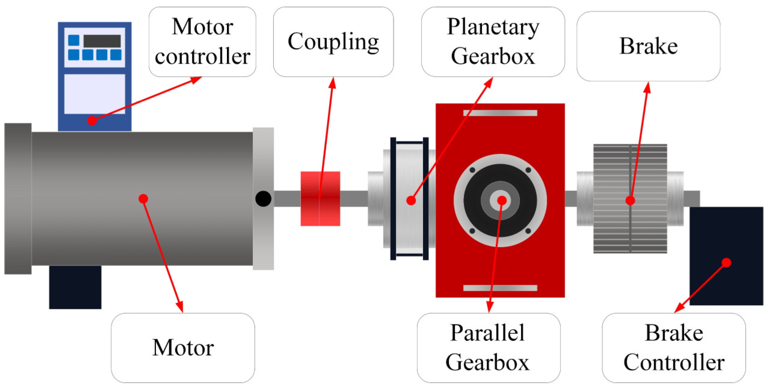
2. Experimental Setup

The validation experiments are carried out using the Southeast University (SEU) bearing dataset and the Case Western Reserve University (CWRU) bearing dataset. The experiments are mainly divided into two parts: contrast experiments on other bearing fault diagnosis methods and ablation experiments to verify the role of each key innovation point. To reduce the random initialization, the experiment was repeated 10 times in every case.

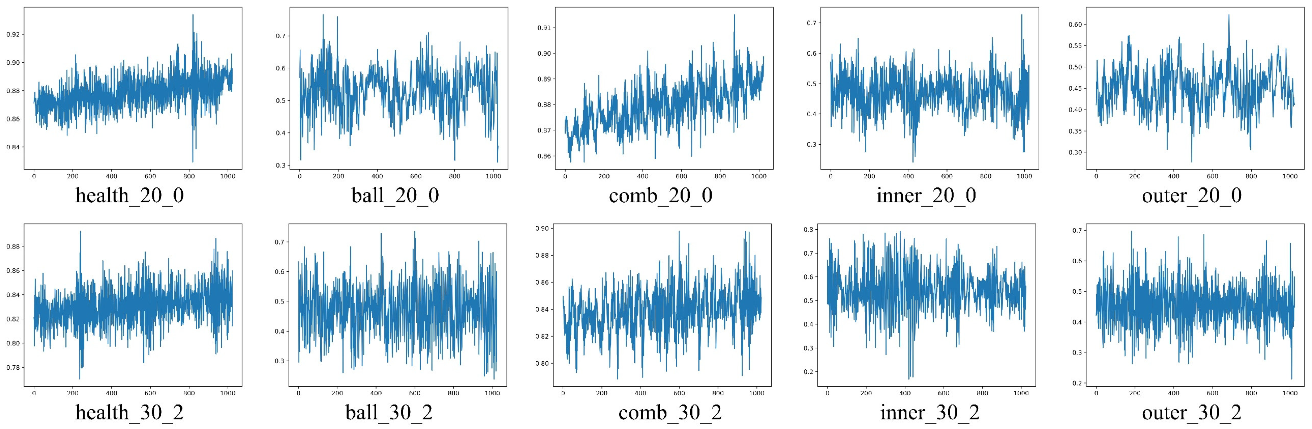
2.1. Dataset Information

The first bearing dataset was provided by the SEU of China [34], which included the vibration data of bearings and gears. As shown in Figure 1, the test configuration consists of a motor, a motor controller, a planetary gearbox, a reduction gearbox, a brake, and a brake controller. The vibration signals were sampled at 5120 Hz and contained five different bearing conditions: ball fault, inner ring fault, outer ring fault, combination fault on both inner ring and outer ring, and normal operation. Each fault type corresponds to two working conditions: speed 20 Hz (1200 rpm), load 0 V (0 Nm) and speed 30 Hz (1800 rpm), load 2 V (7.32 Nm). It is noted that diagnosing bearing fault is a 10-step classification task. Each sample length in the dataset was divided into 1024 data points. A total of 100 samples were randomly selected for each health state, and the ratio of the training set to the validation set was 3:1.

The second bearing dataset was obtained from Case Western Reserve University (CWRU) Electrotechnics Lab [18]. The experimental subject of the CWRU dataset was the deep furrow ball bearing SKF6205 (Figure 2). The test bench consisted of a 1.5 kW motor, a torque sensor, a power tester, and control electronics. The motor speeds were 1772 rpm, 1750 rpm, and 1730 rpm, which corresponded to loads of 1 hp, 2 hp, and 3 hp, respectively. Vibration signal data were collected for normal bearing, single point drive, and fan end defects. The acceleration sensor was used to collect signals in the experiment. The frequency of digital signal acquisition was 12 kHz and 48 kHz. In this work, the vibration signal of the driving end was applied, and the sampling frequency was set at 12 kHz. Bearings had a total of ten conditions, including one normal state and nine fault states. The original dataset file recorded 10 bearing vibration data corresponding to 10 categories of bearing states. Each data file contained approximately 256,000 data points, and each generated sample contained 1024 data points. Similar to the SEU dataset above, 100 samples were randomly selected for each health condition, and the ratio of the training set to the validation set was 3:1.

As illustrated in Figure 3 and Figure 4 (time-domain waveforms), the raw signals from faulty bearings display distinct impulse patterns (e.g., amplitude modulation at characteristic fault frequencies). While these features permitted preemptive fault detection, accurate classification (e.g., distinguishing between inner and outer race defects) necessitated the advanced feature extraction capabilities provided by our MGE-ResNet framework.

The SEU and CWRU bearing datasets employed in this study contain both single crack faults (inner race, outer race, rolling element) and compound faults (concurrent inner/outer race cracks). Importantly, these artificially machined cracks induced multiplicative faults through modulation mechanisms [35,36], where the defect-induced vibrations amplitude-modulated the healthy carrier signal. For complex faults, multiple cracks simultaneously generated superimposed modulation effects, with each defect contributing independent sideband components to the vibration spectrum. It is also noted that both the SEU and CWRU bearing datasets used in this study were collected offline and did not support real-time monitoring; therefore, the experimental analysis was mainly based on historical data.

2.2. Methods

Our developed fault diagnosis network model was derived from the combination of ResNet with multiscale, the Ghost module, and lightweight Efficient Channel Attention (ECA) mechanism (ResNet-Multi-Ghost-ECA). For simpler expression, we will use ResNet-Multi-Ghost-ECA as MGE-ResNet hereafter.

2.2.1. Design of MGE-ResNet

Figure 5 demonstrates the overall framework of the developed multiscale lightweight deep learning model (MGE-ResNet). This diagnostic approach mainly involves three important steps. First, the dimension of bearing vibration timing signals is improved by adopting Gramian Angular Field coding, and Gramian angular summation field (GASF) images. In this step, a set of time series data is converted into spatial image information, which can reveal the internal structure and changes in the laws of the data. Second, the Gaussian pyramid method is employed to process GASF images, and the feature images of different scales are obtained. Third, the proposed GE block, which consists of the Ghost module and ECA module, can extract lightweight features and perform adaptive weight processing on the features. This system can allow for the representation ability of key features at various scales. The final features extracted at different scales are then fused through feature concatenation, and the bearing fault classification is completed through the fully connected network.

2.2.2. Gramian Angular Field (GAF) Encoding

The GAF method converts a one-dimensional (1-D) time domain signal into a two-dimensional (2-D) image by Gram matrix calculation. GAF preserves the global information of the original data and has the advantage of not being limited by the resolution of the frequency domain and not relying on the time window. The linear mapping method is used to normalize 1-D bearing vibration signals to ensure that all values are on the same scale. Then, the normalized vibration signals are scaled down using polar coordinates as follows:

$$\left\{\begin{array}{c}\phi =arccos x_i, -1\ll x_i\ll 1\\ r=t_i/L \end{array}\right.$$

(1)

where $\phi$ is the polar angle in polar coordinates, $x_i$ is the vibration signal value after normalization, $r$ is the polar diameter in polar coordinates, $t_i$ is the time step, $L$ is the constant factor under the polar coordinate notation, and $i$ is the sampling point.

As these polar coordinates contain the amplitude and phase information of the vibration signal, the internal characteristics can be characterized according to the obtained polar coordinates. The relationship between different sampling points can be established by using the sine and cosine functions. Among them, the feature map encoded by the cosine function is called the Gramian Angular Summation Field (GASF). The feature map encoded by the sine function is called the Gramian Angular Difference Field (GADF). GASF is a symmetric square matrix and its corresponding GADF is an antisymmetric square matrix. In this study, we use GASF to encode the bearing vibration signals. For a given time-domain vibration signal, its corresponding GASF can be calculated as follows:

$$GASF=\cos ({\phi }_i+{\phi }_j)$$

(2)

where ${\phi }_i$ and ${\phi }_j$ are the polar angles of the $i$ and $j$ sampling points in polar coordinates, respectively.

2.2.3. Ghost Module

The network principle of Ghost Module is to split the one-time convolution calculation of traditional convolution into two steps: ordinary convolution and simple linear calculation (Figure 6). A small number of feature maps are first generated via an ordinary convolution according to the following equation:

$$F=X\ast W+b$$

(3)

where $F$ is the generated basic feature map, $X$ is the input data, $W$ is the weight of the convolution kernel, $b$ is the bias of the convolution operation, and $\ast$ indicates a convolution operation.

The second step is to generate additional feature maps by performing a series of computationally less expensive operations, such as linear transformations, average pooling, depth curling, etc. These additional feature maps, called Ghost feature maps, do not result in extensive computational effort and are calculated as follows:

$$A_i={\mathsf{\Phi }}_i\left(F_i;{\theta }_i\right), i=1, 2,\dots ,k$$

(4)

where $A_i$ is the i-th additional feature map generated by low-cost computation, $F_i$ is the i-th basic feature map, ${\mathsf{\Phi }}_i$ represents the low-cost computation, ${\theta }_i$ is the parameter for the low-cost computation, and $k$ represents the number of additional feature maps that need to be generated.

Then, the same number of feature maps as the traditional convolutional output is obtained by combining similar feature maps and previously generated feature maps with identical changes. The output feature maps are calculated as follows:

$$O=[F, A_1,A_2,\dots ,A_k]$$

(5)

2.2.4. Efficient Channel Attention (ECA) Module

Figure 7 shows the overall configuration of the ECA module. ECA first runs the input feature map through the global average pooling layer to obtain aggregate features. The weight of each channel is then obtained by the Sigmoid activation function using a 1-D convolution with the convolution kernel size $k=\psi \left(c\right)$, where $k$ is dynamically calculated according to the number of channels $c$ in the input feature map. Finally, the weight value is multiplied by the corresponding elements of the original input feature map to obtain the final output feature map (i.e., Hadamard product—known as an element-wise product).

ECA utilizes 1-D convolution to implement the interaction between channels. The Sigmoid activation function is used to assign weights to each channel feature, which improves the recognition ability of important features and inhibits the interference of non-important features. ECA eliminates the need for a dimensionality reduction operation, prevents the loss of important features, and improves the efficiency of feature extraction.

2.2.5. GE (Ghost and ECA) Block

The GE block is constructed using the Ghost and ECA modules (Figure 8). The GE block is a bottleneck structure composed of two Ghost module layers. The overall structure of the GE block is very similar to that of the Residual block. One might think of it as a direct replacement of the normal convolution operation of the Residual block with the Ghost Module. To improve the ability to extract key features, the ECA module is introduced to the second Ghost module. The improved network not only ensures the accuracy of model detection but also greatly reduces the number of parameters and calculation complexity of the model.

2.2.6. Multiscale Feature Fusion

To improve the ability of multiscale feature extraction, the Gaussian pyramid method is employed to process GASF images. The size of an input GASF image $I_0$ is $s_0=w\times h$. As the scale level increases, the image size is reduced by half. Thus, the size of the image $I_l$ on the scale level $l$ is

$$s_l=w/2^l\times h/2^l, l\in \left\{\mathrm{0,1},\dots ,n\right\}.$$

(6)

Multiscale pyramid images of different scales are obtained as $L=\left\{I_l| 0\le l\le n\right\}$. In this study, GASF images of three different scales were obtained. For each scale, we designed different neural network branches. For scale = 0, we used 4-layer GE blocks to ensure the adequacy of feature extraction. For scale = 1, we used 3-layer GE blocks to ensure the adequacy of feature extraction. For scale = 2, we used 2-layer GE blocks to ensure the adequacy of feature extraction. The final features extracted at different scales were fused through feature concatenation. Finally, the bearing fault classification was completed through the fully connected network.

3. Results

To demonstrate the efficiency of our system, several experiments were conducted, and the results were analyzed based on different performance metrics. In addition, the feature learning capability of the proposed model was verified using the T-distributed stochastic neighbor embedding (T-SNE) technique.

3.1. Validation of Datasets

Based on the two datasets above, our developed MGE-ResNet approach was employed to validate the performance using two main experiments (i.e., contrast and ablation). To verify the performance of MGE-ResNet, we compared it with five other typical intelligent fault-diagnosis methods for bearings, namely SVM [34], TICNN [37,38], Ni-Net [39], Improved AlexNet [40], and SE-ResNet152 [24]. SVM uses standard Support Vector Machines for bearing fault diagnosis, denoted as Method_1. TICNN (Convolution Neural Networks with Training Interference) is an enhanced CNN (Convolution Neural Network) model, denoted as Method_2. Ni-Net (Noise ignoring Network) is a bearing fault-diagnosis model based on VGG-16 (Visual Geometry Group), denoted as Method_3. Improved AlexNet, a typical bearing fault diagnosis algorithm enhanced by Alexnet, is denoted as Method_4. SE-ResNet152, a typical bearing fault-diagnosis algorithm based on ResNet, is denoted as Method_5. During the training process, the batch size was set to 16, the number of iterations was set to 40. The adopted optimizer was Stochastic Gradient Descent (SGD). The learning rate was then determined by using the grid search method. It is noted that each experiment was repeated 10 times to minimize the random initialization.

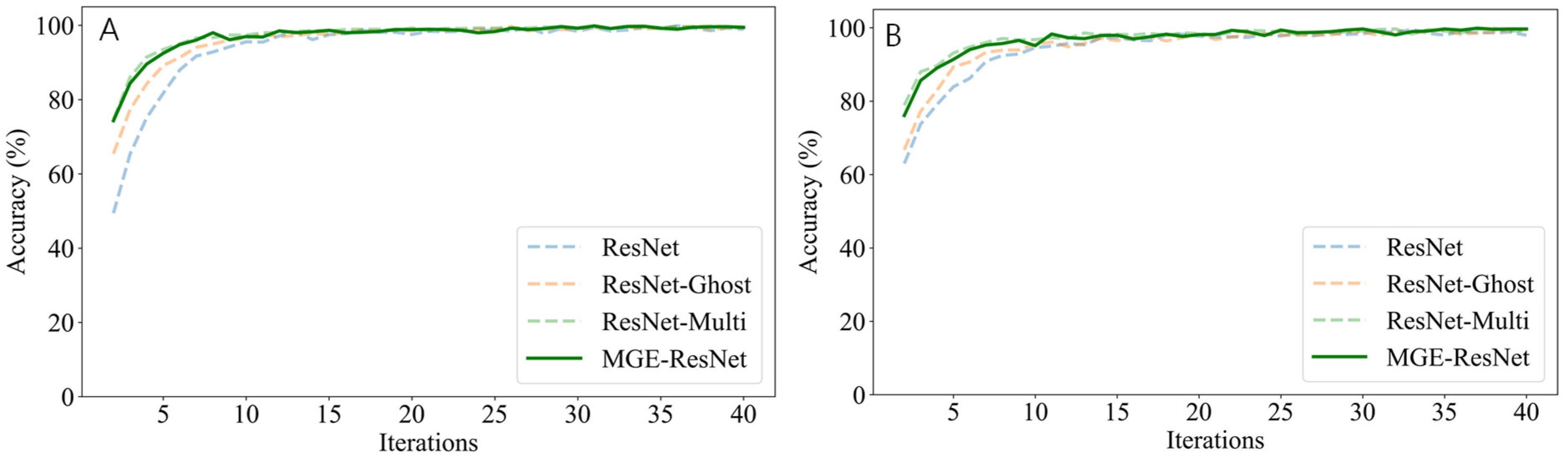
3.2. Contrast Experiment

To comprehensively evaluate the performance of the MGE-ResNet approach, the experimental study adopts the following metrics across three dimensions—classification accuracy, robustness, and computational efficiency—for comparative analysis.

(1)

Accuracy

It measures the overall prediction accuracy, particularly suitable for balanced class distributions:

$$\mathrm{A}\mathrm{c}\mathrm{c}\mathrm{u}\mathrm{r}\mathrm{a}\mathrm{c}\mathrm{y}=(\mathrm{T}\mathrm{P}+\mathrm{T}\mathrm{N})/(\mathrm{T}\mathrm{P}+\mathrm{T}\mathrm{N}+\mathrm{F}\mathrm{P}+\mathrm{F}\mathrm{N})$$

(7)

where TP (true positive) denotes correctly classified faulty samples, TN (true negative) represents correctly identified normal samples, FP (false positive) indicates normal samples misclassified as faults, and FN (false negative) represents undetected faulty samples.

(2)

Recall and Precision

Recall emphasizes fault detection capability to minimize missed alarms:

$$\mathrm{R}\mathrm{e}\mathrm{c}\mathrm{a}\mathrm{l}\mathrm{l}=\mathrm{T}\mathrm{P}/(\mathrm{T}\mathrm{P}+\mathrm{F}\mathrm{N})$$

(8)

Precision focuses on prediction reliability to reduce false alarms:

$$\mathrm{P}\mathrm{r}\mathrm{e}\mathrm{c}\mathrm{i}\mathrm{s}\mathrm{i}\mathrm{o}\mathrm{n}=\mathrm{T}\mathrm{P}/(\mathrm{T}\mathrm{P}+\mathrm{F}\mathrm{P})$$

(9)

(3)

F1 Score

The F1 score harmonizes recall and precision through harmonic mean:

$$\mathrm{F}1=2·\mathrm{P}\mathrm{r}\mathrm{e}\mathrm{c}\mathrm{i}\mathrm{s}\mathrm{i}\mathrm{o}\mathrm{n}·\mathrm{R}\mathrm{e}\mathrm{c}\mathrm{a}\mathrm{l}\mathrm{l}/(\mathrm{P}\mathrm{r}\mathrm{e}\mathrm{c}\mathrm{i}\mathrm{s}\mathrm{i}\mathrm{o}\mathrm{n}+\mathrm{R}\mathrm{e}\mathrm{c}\mathrm{a}\mathrm{l}\mathrm{l})$$

(10)

(4)

GFLOPs (Giga Floating-Point Operations)

GFLOPs quantify the computational complexity of a deep learning model by measuring the number of floating-point operations (FLOPs) required for a single forward pass. Higher GFLOPs indicate that the total amount of floating-point operations required for model execution is higher. High GFLOPs typically require a significant amount of hardware resources and may not be suitable for real-time response scenarios:

$$\mathrm{G}\mathrm{F}\mathrm{L}\mathrm{O}\mathrm{P}\mathrm{s}={\displaystyle \frac{1}{{10}^9}}{\sum }_{l=1}^{\mathrm{L}}\left(2·{\mathrm{C}}_l^{\mathrm{i}\mathrm{n}}·{\mathrm{K}}_l^2·{\mathrm{C}}_l^{\mathrm{o}\mathrm{u}\mathrm{t}}·{\mathrm{H}}_l·{\mathrm{W}}_l\right)$$

(11)

where L is the total number of convolutional layers, ${\mathrm{C}}_l^{\mathrm{i}\mathrm{n}}$/${\mathrm{C}}_l^{\mathrm{o}\mathrm{u}\mathrm{t}}$ is the input/output channels of the l-th layer, K_l is the spatial size of the convolutional kernel, ${\mathrm{H}}_l$ is the height of the output feature map, and ${\mathrm{W}}_l$ is the width of the output feature map.

The average fault diagnosis accuracy using the MGE-ResNet approach and the other five typical methods is displayed in

Table 2. Experimental comparison of the average fault diagnosis accuracy.

Method	Experiment 1		Experiment 2
	Average Accuracy (%)	GFLOPs	Average Accuracy (%)	GFLOPs
Method_1	81.46 ± 4.28	0.48	86.88 ± 2.15	0.48
Method_2	88.50 ± 8.14	0.69	71.54 ± 7.68	0.69
Method_3	96.81 ± 3.05	30.83	93.67 ± 5.46	30.83
Method_4	97.94 ± 1.91	1.88	97.58 ± 2.10	1.88
Method_5	95.65 ± 4.22	4.21	93.31 ± 6.85	4.21
MGE-ResNet	99.44 ± 0.42	1.99	99.54 ± 0.46	1.99

Note: Method_1: SVM, Method_2: TICNN, Method_3: Ni-Net, Method_4: improved AlexNet, Method_5: SE-ResNet152.

. It has revealed that our method achieved the highest fault diagnosis accuracy on both SEU and CWRU bearing datasets. For example, MGE-ResNet reached the average accuracies of 99.44% and 99.54% on the SEU and CWRU datasets, respectively. However, SVM (Method_1) achieved accuracies of 81.46% and 86.88% on the same datasets, revealing a notable performance gap. This disparity could stem from the reliance of SVM on manual feature engineering (e.g., extracting 12 time/frequency-domain features including kurtosis, RMS, and spectral entropy) versus the capability of MGE-ResNet to automatically learn discriminative multiscale representations directly from the raw signals. Based on the SEU dataset, MGE-ResNet generally outperformed Method_1 by 17.98%, Method_2 by 10.94%, Method_3 by 2.63%, Method_4 by 1.5%, and Method_5 by 3.79%. A similar trend was also obtained using the CWRU bearing dataset. In addition, the deviation of fault diagnosis accuracy was also the smallest among all other methods based on 10 randomized experiments. Comparing the GFLOPs values, our approach improved accuracy while maintaining a sufficient level of lightweight features. Thus, the method we developed in this work presents high accuracy with minimal variations in fault diagnosis, which can fully fulfill the actual engineering needs of bearing fault diagnosis.

Figure 9 shows the effects of training iterations on these different methods in Experiment 1 and Experiment 2. Method_5 and MGE-ResNet showed significantly higher initial accuracy (%) than the other three Methods (1–4). In addition, Method_5 and MGE-ResNet displayed similar patterns, with the accuracy converging quickly as the number of iterations increased, whereas the other four methods exhibited a gradual increase in accuracy. The results revealed that our MGE-ResNet model achieved the fastest convergence speed and the highest accuracy on both the SEU bearing dataset and the CWRU dataset. In both experiments using two datasets, it was clearly observed that our method maintained the highest bearing fault diagnosis accuracy and stability after rapid convergence.

The performance of the bearing fault diagnosis methods was considered in four different metrics: accuracy, F1 score, recall, and precision are shown in Figure 10. The results clearly revealed that the comprehensive performance of the proposed method is superior to other comparative methods, and it achieves the best balance between accuracy and model lightweight level, which can fully fulfill the actual engineering needs.

Figure 11 shows the confusion matrix of MGE-ResNet in Experiment 1 (A) and Experiment 2 (B). From this observation, it was found that the proposed MGE-ResNet accurately identified the 10 classes of bearing faults on the two different datasets.

3.3. Ablation Experiment

Ablation experiments were also designed to validate the significant role of each key module. Taking ResNet as the base method, the impact of each key module on the overall performance of the method proposed in this paper was evaluated by gradually introducing other modules. The specific comparison methods utilized in this study include ResNet, ResNet-Ghost, ResNet-Multi-Ghost, and ResNet-Multi-Ghost-ECA. While ResNet utilizes a simple deep learning model (i.e., Residual Neural Network) to identify rolling bearing faults by examining vibrational signals, ResNet-Ghost added the Ghost module to reduce feature redundancy and improve computational efficiency. ResNet-Multi-Ghost combines multiscale feature fusion with the Ghost module to further enhance diagnostic performance and computational efficiency. Lastly, ResNet-Multi-Ghost-ECA aims to enhance the information interaction and weight allocation among channels by introducing the ECA mechanism based on the above model. Thus, the fault diagnosis effectiveness of each method was compared based on the test set using the average accuracy, iteration accuracy of different methods, and average F1 score.

The ablation experimental results of the four contrasting methods on two evaluation metrics, such as average fault diagnosis accuracy and GFLOPs, are presented in

Table 3. Ablation experimental comparison of the average fault diagnosis accuracy.

Method	Experiment 1		Experiment 2
	Average Accuracy (%)	GFLOPs	Average Accuracy (%)	GFLOPs
ResNet	98.64 ± 1.42	3.60	97.95 ± 1.85	3.60
ResNet-Ghost	98.62 ± 2.16	1.81	98.42 ± 0.92	1.81
ResNet-Multi-Ghost	98.91 ± 1.91	1.99	99.25 ± 0.66	1.99
MGE-ResNet	99.44 ± 0.42	1.99	99.54 ± 0.46	1.99

. Although the overall accuracy of fault diagnosis was comparable between ResNet and ResNet-Ghost, the average diagnosis accuracy of ResNet-Multi-Ghost achieved a certain level of improvement in both Experiment 1 and Experiment 2 after the simultaneous adoption of multiscale feature fusion and the Ghost module. When introducing the additional ECA mechanism, the average fault diagnosis accuracy of our approach (i.e., MGE-ResNet) was further improved with stability. After the introduction of the Ghost module, ResNet-Ghost notably reduced GFLOPs compared to ResNet (from 3.60 to 1.81). This observation proves that the Ghost module helps to raise the level of lightness of the model. After the introduction of multiscale feature fusion and the ECA mechanism, the GFLOPs of ResNet-Multi-Ghost and MGE-ResNet were slightly increased by 0.18 compared to ResNet-Ghost. This demonstrates that the utilization of multiscale feature fusion and the ECA mechanism could slightly increase model complexity but meaningfully improve the fault diagnosis accuracy.

Figure 12 shows the effects of the training iterations on the four different methods using Experiment 1 and Experiment 2 datasets. The ablation experimental results revealed that ResNet18 and ResNet18-Ghost generally showed detectably lower initial accuracy (%). However, ResNet-Multi-Ghost and MGE-ResNet exhibited comparable accuracy patterns with increasing the number of iterations and the highest convergence speed and accuracy on the SEU bearing and CWRU datasets. Again, our developed approach still maintained the highest bearing fault diagnosis accuracy and stability at the same time after fast convergence.

Lastly, the feature learning capability of the proposed model was verified using the T-distributed stochastic neighbor embedding (t-SNE) technique shown in Figure 13 and Figure 14. The t-SNE method is often employed to illustrate the feature extraction capabilities of different methods, providing a clearer comparison of their effectiveness in distinguishing different fault types that are presented in Figures (“Outer” represents outer race faults, “Inner” represents inner race faults, “Norm” denotes normal bearings, “Ball” refers to ball faults, and “Comb” indicates compound faults). By comparing the feature visualization results of our developed method and the rest of the approaches, it is evident that the MGE-ResNet exhibited a stronger clustering effect. This improvement was attributed to the use of the GAF matrix representation of the raw signals, which transformed the time-series data into structured images. The incorporation of multiscale feature fusion further enhanced the ability of the network to capture critical fault characteristics across different scales, leading to more discriminative feature representations. These t-S NE visualizations enhance the interpretability of our model’s classification results, which could provide a more intuitive understanding of how different fault types are distinguished in the learned feature space.

4. Conclusions

In this work, we demonstrated a multiscale lightweight deep learning method (MGE-ResNet) to resolve the problem of existing methods that make it difficult to simultaneously consider the accuracy and lightweight in bearing fault diagnosis. The key technical contributions of MGE-ResNet include four main points. First, the Gaussian pyramid method is utilized to express the Gramian Angular Summation Field (GASF) matrix image in multiple scales generated by the time-series signal transformation of bearing vibration. This approach effectively improves the quality of feature representation. Second, the Ghost module is employed to replace the traditional convolution operation, which effectively enhances the computational efficiency and lightweight level of the method. Third, the Efficient Channel Attention (ECA) module is used to extract the dependencies between different feature channels to enhance the expression capability of key features. This addition effectively improves the learning ability of bearing fault features and increases the accuracy of fault diagnosis. Lastly, the residual module GE block is built based on the Ghost module and ECA, which are integrated into the backbone network. The effectiveness of the developed method is verified using two different bearing fault diagnosis datasets. The experimental results evidently show that the comprehensive performance of our bearing fault diagnosis method is better than the other four conventional methods. Considering the optimal balance between accuracy and lightweight model, our approach can sufficiently meet the needs of practical applications. Although the pre-damaged bearing approach enabled controlled fault characterization, this method did not capture dynamic fault progression. Future studies will involve the incorporation of run-to-failure datasets to validate temporal sensitivity.

References

1. Bai, Y.; Cheng, W.; Wen, W.; Liu, Y. Application of time-frequency analysis in rotating machinery fault diagnosis. Shock Vib. 2023, 2023, 9878228. [Google Scholar] [CrossRef]
2. Kankar, P.K.; Sharma, S.C.; Harsha, S.P. Fault diagnosis of ball bearings using machine learning methods. Expert Syst. Appl. 2011, 38, 1876–1886. [Google Scholar] [CrossRef]
3. Ahmad, H.; Cheng, W.; Xing, J.; Wang, W.; Du, S.; Li, L.; Zhang, R.; Chen, X.; Lu, J. Deep learning-based fault diagnosis of planetary gearbox: A systematic review. J. Manuf. Syst. 2024, 77, 730–745. [Google Scholar] [CrossRef]
4. He, M.; He, H. Deep learning based approach for bearing fault diagnosis. IEEE Trans. Ind. Appl. 2017, 53, 3057–3065. [Google Scholar] [CrossRef]
5. Cai, Y.-P.; Li, A.-H.; Shi, L.-S.; Bai, X.-F.; Shen, J.-W. Roller bearing fault detection using improved envelope spectrum analysis based on EMD and spectrum Kurtosis. J. Vib. Shock. 2011, 30, 167–172. [Google Scholar]
6. Dragomiretskiy, K.; Zosso, D. Variational mode decomposition. IEEE Trans. Signal Process. 2014, 62, 531–544. [Google Scholar] [CrossRef]
7. Hu, A.-J.; Ma, W.-L.; Tang, G.-J. Rolling bearing fault feature extraction method based on ensemble empirical mode decomposition and Kurtosis criterion. Proc. Chin. Soc. Electr. Eng. 2012, 32, 106–111. [Google Scholar]
8. Zhao, H.; Guo, S.; Gao, D. Singular value decomposition and variational modal decomposition based  Fault feature extraction of bearing fault. J. Vib. Shock 2016, 35, 183–188. [Google Scholar]
9. Tang, Z.; Wang, M.; Ouyang, T.; Che, F. A wind turbine bearing fault diagnosis method based on fused depth features in time–frequency domain. Energy Rep. 2022, 8, 12727–12739. [Google Scholar] [CrossRef]
10. Tao, H.; Qiu, J.; Chen, Y.; Stojanovic, V.; Cheng, L. Unsupervised cross-domain rolling bearing fault diagnosis based on time-frequency information fusion. J. Frankl. Inst. 2023, 360, 1454–1477. [Google Scholar] [CrossRef]
11. Xie, F.; Li, G.; Song, C.; Song, M. The early diagnosis of rolling bearings’ faults using fractional Fourier transform information fusion and a lightweight neural network. Fractal Fract. 2023, 7, 875. [Google Scholar] [CrossRef]
12. Zou, F.; Zhang, H.; Sang, S.; Li, X.; He, W.; Liu, X. Bearing fault diagnosis based on combined multi-scale weighted entropy morphological filtering and bi-LSTM. Appl. Intell. 2021, 51, 6647–6664. [Google Scholar] [CrossRef]
13. Lei, M.; Meng, G.; Dong, G. Fault detection for vibration signals on rolling bearings based on the symplectic entropy method. Entropy 2017, 19, 607. [Google Scholar] [CrossRef]
14. Binti Shahrulhisham, N.N.H.; Chong, K.H.; Yaw, C.T.; Koh, S.P. Application of machine learning technique using support vector machine in wind turbine fault diagnosis. J. Phys. Conf. Ser. 2022, 2319, 012017. [Google Scholar] [CrossRef]
15. An, X.L.; Jiang, D.X.; Li, S.H.; Chen, J. Fault diagnosis of direct-drive wind turbine based on support vector machine. J. Phys. Conf. Ser. 2011, 305, 012030. [Google Scholar] [CrossRef]
16. Huang, Y. Fault diagnosis of spindle bearing in wind turbine based SVM. Instrumentation 2016, 23, 88–92. [Google Scholar]
17. Xu, Y.-G.; Meng, Z.-P.; Lu, M. Fault diagnosis method of rolling bearing based on dual-tree complex wavelet packet transform and SVM. J. Aerosp. Power 2014, 29, 67–73. [Google Scholar]
18. Xin, W.; Yan, W.-Y. Fault diagnosis of roller bearings based on variational mode decomposition and SVM. J. Vib. Shock 2017, 36, 252–256. [Google Scholar]
19. Lei, N.; Huang, F.; Li, C. Rolling bearing fault diagnosis based on variational mode decomposition and weighted multidimensional feature entropy fusion. J. Vibroeng. 2024, 26, 590–614. [Google Scholar] [CrossRef]
20. Li, L.; Meng, W.; Liu, X.; Fei, J. Research on rolling bearing fault diagnosis based on variational modal decomposition parameter optimization and an improved support vector machine. Electronics 2023, 12, 1290. [Google Scholar] [CrossRef]
21. Gao, L.X.; Ren, Z.Q.; Zhang, J.Y.; Xu, Y.G.; Wang, Y. Rolling bearing fault diagnosis methods based on Fisher ratio and SVM. J. Beijing Univ. Technol. 2011, 37, 13–18. [Google Scholar]
22. Cheng, J.S.; Yu, D.J.; Yang, Y. Fault diagnosis of roller bearings based on EMD and SVM. J. Aerosp. Power 2006, 21, 575–580. [Google Scholar]
23. Guan, X.; Chen, G. Sharing pattern feature selection using multiple improved genetic algorithms and its application in bearing fault diagnosis. J. Mech. Sci. Technol. 2019, 33, 129–138. [Google Scholar] [CrossRef]
24. Wu, G.; Ji, X.; Yang, G.; Jia, Y.; Cao, C. Signal-to-image: Rolling bearing fault diagnosis using ResNet family deep-learning models. Processes 2023, 11, 1527. [Google Scholar] [CrossRef]
25. Sohaib, M.; Kim, C.-H.; Kim, J.-M. A hybrid feature model and deep-learning-based bearing fault diagnosis. Sensors 2017, 17, 2876. [Google Scholar] [CrossRef]
26. Plakias, S.; Boutalis, Y.S. Fault detection and identification of rolling element bearings with attentive dense CNN. Neurocomputing 2020, 405, 208–217. [Google Scholar] [CrossRef]
27. Liu, X.; Sun, W.; Li, H.; Hussain, Z.; Liu, A. The method of rolling bearing fault diagnosis based on multi-domain supervised learning of convolution neural network. Energies 2022, 15, 4614. [Google Scholar] [CrossRef]
28. Qi, L.; Zhang, Q.; Xie, Y.; Zhang, J.; Ke, J. Research on wind turbine fault detection based on CNN-LSTM. Energies 2024, 17, 4497. [Google Scholar] [CrossRef]
29. Velandia-Cardenas, C.; Vidal, Y.; Pozo, F. Wind turbine gearbox early fault detection using Mel-Frequency Cepstral Coefficients of vibration data. Struct. Control Health Monit. 2024, 2024, 7733730. [Google Scholar] [CrossRef]
30. Wang, C.; Li, D. Fault early warning of fan gearbox bearing based on LSTM network. Electr. Power Sci. Eng. 2020, 36, 40–45. [Google Scholar]
31. Khorram, A.; Khalooei, M.; Rezghi, M. End-to-end CNN + LSTM deep learning approach for bearing fault diagnosis. Appl. Intell. 2021, 51, 736–751. [Google Scholar] [CrossRef]
32. Han, K.; Wang, Y.; Tian, Q.; Guo, J.; Xu, C.; Xu, C. Ghostnet: More features from cheap operations. In Proceedings of the 2020 IEEE/CVF Conference on Computer Vision and Pattern Recognition, Seattle, WA, USA, 13–19 June 2020; pp. 1580–1589. [Google Scholar]
33. Wang, Q.; Wu, B.; Zhu, P.; Li, P.; Zuo, W.; Hu, Q. ECA-Net: Efficient channel attention for deep convolutional neural networks. In Proceedings of the 2020 IEEE/CVF Conference on Computer Vision and Pattern Recognition, Seattle, WA, USA, 13–19 June 2020; pp. 11534–11542. [Google Scholar]
34. Li, C.; Mo, M.; Yan, R. Fault diagnosis of rolling bearing based on WHVG and GCN. IEEE Trans. Instrum. Meas. 2021, 70, 3519811. [Google Scholar] [CrossRef]
35. Juhlin, M.; Sward, J.; Pesavento, M.; Jakobsson, A. Estimating faults modes in ball bearing machinery using a sparse reconstruction framework. In Proceedings of the 2018 26th European Signal Processing Conference (EUSIPCO), Rome, Italy, 3–7 September 2018; pp. 2330–2334. [Google Scholar]
36. Pang, B.; He, Y.; Tang, G.-J.; Zhou, C.; Tian, T. Rolling bearing fault diagnosis based on optimal notch filter and enhanced singular value decomposition. Entropy 2018, 20, 482. [Google Scholar] [CrossRef] [PubMed]
37. Zhang, W.; Li, C.; Peng, G.; Chen, Y.; Zhang, Z. A deep convolutional neural network with new training methods for bearing fault diagnosis under noisy environment and different working load. Mech. Syst. Signal Process. 2018, 100, 439–453. [Google Scholar] [CrossRef]
38. Jin, Z.; Chen, D.; He, D.; Sun, Y.; Yin, X. Bearing fault diagnosis based on VMD and improved CNN. J. Fail. Anal. Prev. 2023, 23, 165–175. [Google Scholar] [CrossRef]
39. Huang, J. Deep-learning-based rolling element bearing fault diagnosis considering noise utilizing enhanced VGG-16. In Proceedings of the 2024 IEEE 6th International Conference on Power, Intelligent Computing and Systems (ICPICS), Shenyang, China, 26–28 July 2024; pp. 1547–1552. [Google Scholar]
40. Mohiuddin, M.; Islam, M.S.; Islam, S.; Miah, M.S.; Niu, M.-B. Intelligent fault diagnosis of rolling element bearings based on modified AlexNet. Sensors 2023, 23, 7764. [Google Scholar] [CrossRef]
Figure 1. Test equipment of the SEU dataset.
Processes 13 01239 g001
Figure 2. Test equipment of the CWRU dataset.
Processes 13 01239 g002
Figure 3. Time-domain signal of faulty bearings for the SEU dataset. Note: X-axis for time sequence (5.12 kHz sampling) and Y-axis for normalized vibration acceleration (g).
Processes 13 01239 g003
Figure 4. Time-domain signal of faulty bearings for the CWRU dataset. Note: X-axis for time sequence (12 kHz sampling) and Y-axis for normalized vibration acceleration (g).
Processes 13 01239 g004
Figure 5. Overall framework of the MGE-ResNet.
Processes 13 01239 g005
Figure 6. A diagram of the Ghost module.
Processes 13 01239 g006
Figure 7. A diagram of the ECA module.
Processes 13 01239 g007
Figure 8. A diagram of the GE (Ghost and ECA) block.
Processes 13 01239 g008
Figure 9. Iterative accuracy of different methods using the Experiment 1 (A) and Experiment 2 (B) datasets.
Processes 13 01239 g009
Figure 10. Indicator performance of different methods in Experiment 1 (A) and Experiment 2 (B).
Processes 13 01239 g010
Figure 11. The confusion matrix diagram of MGE-ResNet in Experiment 1 (A) and Experiment 2 (B).
Processes 13 01239 g011
Figure 12. Iterative accuracy in ablation by four different methods using Experiment 1 (A) and Experiment 2 (B) datasets.
Processes 13 01239 g012
Figure 13. The feature adaptation results of the t-SNE in the ablation experiment using the SEU dataset. Note: “Outer”—outer race faults, “Inner”—inner race faults, “Health”—normal bearings, “Ball”—ball faults, and “Comb”—compound faults.
Processes 13 01239 g013
Figure 14. The feature adaptation results of the t-SNE in the ablation experiment using the CWRU dataset. Note: “Outer”—outer race faults, “Inner”—inner race faults, “Health”—normal bearings, “Ball”—ball faults, and “Comb”—compound faults.
Processes 13 01239 g014