A Numerical Study of Aerodynamic Drag Reduction and Heat Transfer Enhancement Using an Inclined Partition for Electronic Component Cooling

Abstract

This study presents a numerical investigation of fluid flow around a heated rectangular cylinder controlled by an inclined partition, aiming to suppress vortex shedding, reduce aerodynamic drag, and enhance thermal exchange. The double multiple relaxation time lattice Boltzmann method (DMRT-LBM) is employed to investigate the influence of Reynolds number variations and partition positions on the aerodynamic and thermal characteristics of the system. The results reveal the presence of three distinct thermal regimes depending on the Reynolds number. Increasing the Reynolds number intensifies thermal vortex shedding, thereby improving heat exchange efficiency. Moreover, a higher Reynolds number leads to a greater reduction in the drag coefficient, reaching $125.41\%$ for $Re=250$. Additionally, improvements in thermal performance were quantified, with Nusselt number enhancements of $29.47\%$ for $Re=100$, $55.55\%$ for $Re=150, 74.78\%$ for $Re=200$, and $82.87\%$ for $Re=250$. The influence of partition positioning g on the aerodynamic performance was also examined at $Re=150$, revealing that increasing the spacing g generally leads to a rise in the drag coefficient, thereby reducing the percentage of drag reduction. However, the optimal configuration was identified at $g=2d$, where the maximum drag coefficient reduction reached $130.97\%$. In contrast, the impact of g on the thermal performance was examined for $Re=100, 150,$ and $200$, revealing a significant heat transfer improvements on the top and bottom faces: reaching up to $99.47\%$ on the top face for $Re=200$ at $g=3d$. Nevertheless, for all Reynolds numbers and partition placements, a decrease in heat transfer was observed on the front face due to the partition shielding it from the incoming flow. These findings underscore the effectiveness of an inclined partition in enhancing both the thermal and aerodynamic performance of a rectangular component. This approach holds strong potential for various industrial applications, particularly in aeronautics, where similar control surfaces are used to minimize drag, as well as in heat exchangers and electronic cooling systems where optimizing heat dissipation is crucial for performance and energy efficiency.

1. Introduction

Understanding the behavior of airflow around obstacles and optimizing heat transfer mechanisms are crucial aspects in various fields of engineering. In particular, enhancing cooling performance while minimizing aerodynamic drag is a challenge in aerodynamic and thermal management applications, especially for the cooling of electronic components, vehicles, aircraft, construction, etc. To address these challenges, several studies have focused on improving aerodynamic and thermal performances. Gonzalez-Zamudio et al. [1] studied the thermal and dynamic behavior of SiO₂ nanofluid in a lid-driven rectangular cavity using the finite difference method. Their findings provided insights into heat transfer under varying Richardson numbers and wall heating conditions, demonstrating how vortex formation influences convective heat exchange. Elshaer et al. [2] optimized building aerodynamics using a combination of a large eddy simulation (LES) and artificial neural networks (ANNs), achieving a 30% reduction in wind loads through shape modifications. Mena-Pacheco et al. [3] developed a novel methodology for optimizing combined heat and mass exchanger networks (CHAMENs), addressing limitations in thermal and mass exchange integration. Maghrabie et al. [4] explored advanced cooling techniques in microchannel heat sinks (MCHSs) using nanofluids, highlighting improvements in heat dissipation for electronic components. Lv et al. [5] provided an extensive review of thermal management strategies in automotive and aerospace applications, emphasizing the role of active and passive cooling techniques. Xue et al. [6] analyzed heat dissipation in aerospace applications, demonstrating the impact of optimized runner structures on thermal insulation performance.

In addition to these studies, research on passive flow control has explored the use of various control elements, such as flat plates and splitter plates, to alter wake structures and improve heat dissipation. Zhou et al. [7] conducted a two-dimensional numerical analysis to examine the reduction in fluid forces acting on a square cylinder within a channel by implementing an upstream control plate. Their findings indicate that the control plate effectively decreases the drag force on the square cylinder while also attenuating lift fluctuations. Additionally, the study identifies the optimal placement of the control plate for achieving minimal drag depending on its height. In another numerical investigation realized by Islam et al. [8], the fluid flow passed around a square cylinder controlled by a downstream plate at $Re=150$ and $g=0–11$. They also indicated that the drag force achieved a maximum reduction at g = 0, and the optimum space between a square cylinder and the control plate reached at $g=2d$. Turki [9] carried out a numerical investigation for controlling the vortex shedding after a square cylinder for a Reynolds number from 110 through 200 by using a separated flat plate. First, Turki found a linear relationship, $Lc=0.0373\times Re$^–3.4373, characterizing the critical plate length Lc for the vortex shedding disappearance. Likewise, they studied the effect of length and its location of this splitter plate in the wake region on the Strouhal number, and the drag and lift coefficients are analyzed. Dash et al. [10] studied the effect of a dual splitter plate flow separation control device around a square cylinder at a low Reynolds number ($Re$ = 100). Compared to a single plate, this configuration achieves better drag reduction (≈21%) and improved wake control. By varying the plate length and spacing, four distinct flow regimes were identified, with type III being the most effective. Adding more than two plates does not significantly enhance performance. Admi et al. [11] also numerically studied the flow around a square block controlled by four partitions. The researchers positioned the two downstream partitions at a fixed distance of $g=3.9d$, while the two upstream partitions were placed at $g_1=0.25d$, with their length $Lp$ varying between $1d$ and $5d$. Their results indicated that the drag coefficient experienced a maximum reduction of 38.86% when the length of the upstream partitions was set to $2.25d$. Additionally, a maximum vortex shedding suppression is observed in this critical case. Rashidi et al. [12] provided a comprehensive review of both numerical and experimental research on vortex shedding suppression and wake control strategies. They categorized these methods into two primary groups and discussed their respective advantages, limitations, power efficiency, and practical applications.

This present study employs a passive control approach, which involves the use of one or more control elements such as partitions, flat plates, splitters, fins, or rods to influence both flow dynamics and heat exchange. In this work, an inclined partition is strategically placed upstream of a rectangular block to modify the flow structure and enhance thermal performance. Unlike passive control, active control techniques require external energy input, making them more complex to implement and less common in the literature due to their higher operational costs and technical constraints.

Controlling vortex shedding is essential for mitigating fluid-induced forces such as aerodynamic drag and flow-induced vibrations, which directly impact the stability and efficiency of bluff bodies. A numerical study is performed to examine how the presence of an inclined upstream partition affects both the aerodynamic and thermal behavior of a heated rectangular cylinder within a horizontal channel. Unlike conventional passive control strategies that primarily focus on drag reduction, this work introduces an integrated approach that simultaneously addresses vortex shedding suppression, drag minimization, and heat transfer enhancement.

This study contributes a novel perspective to passive flow control by demonstrating the dual benefits of drag reduction and enhanced heat dissipation. The findings offer valuable insights for engineering applications, particularly in aeronautics, where similar control surfaces are utilized to minimize drag, as well as in heat exchanger technologies and electronic cooling systems, where optimizing convective heat transfer is crucial for performance and energy efficiency.

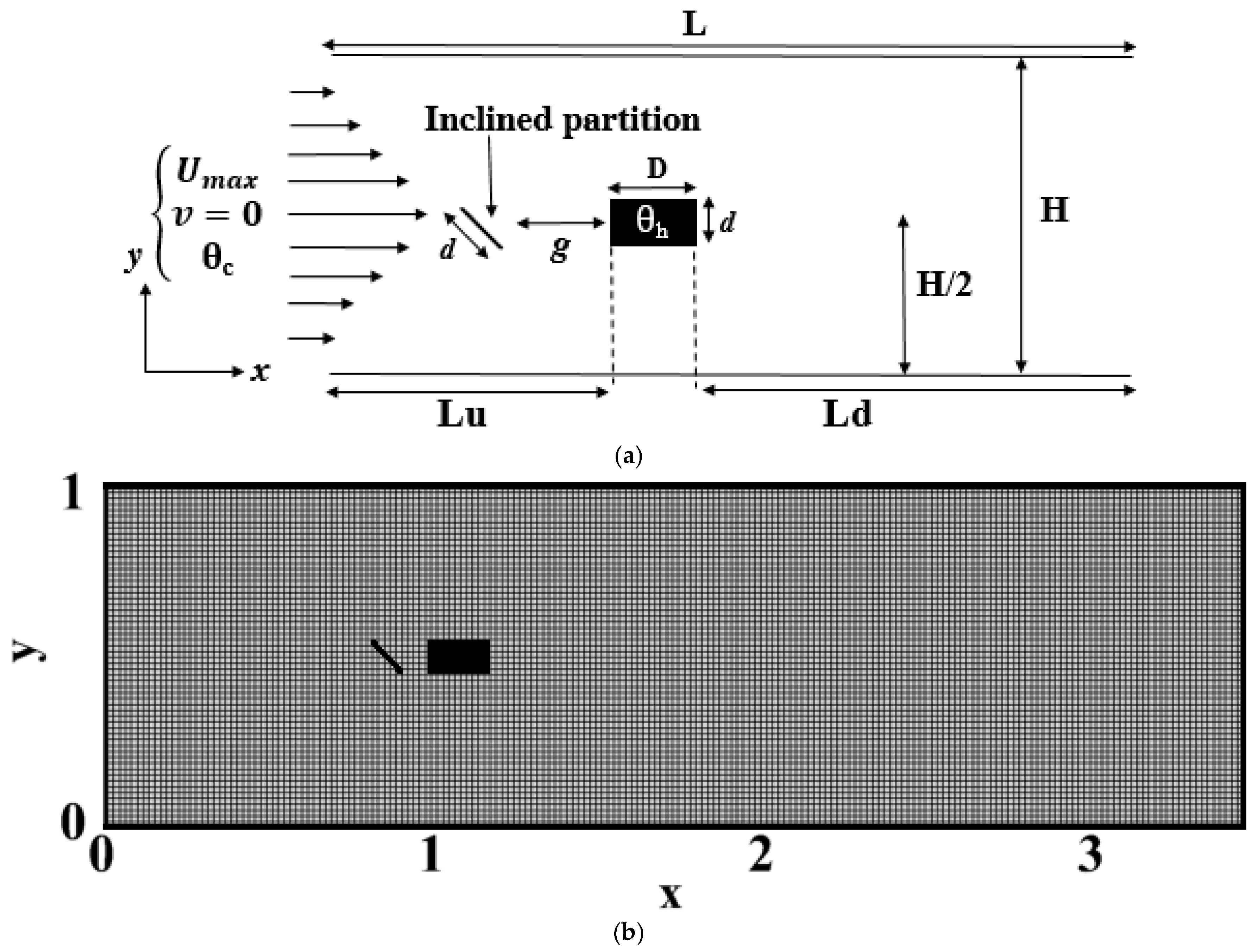
2. Physical Problem

2.1. Geometry Studied

Figure 1a depicts the configuration of the computational domain. Cold air flows around a rectangular block of dimension ($d\times D$) which is located in a two-dimensional channel. The block is located at an upstream distance of $Lu=12d$ and at a downstream distance $Ld=30d$, with a blockage ratio of $\mathsf{\beta }=d/H$ $=1/12$. An inclined partition, of length $Lp=1d$ and height $h=0.25d$, is placed upstream of the block. The spacing between the partition and the cylinder is noted as g.

Figure 1b illustrates the analysis object along with the computational grid used for numerical simulations. The object, consisting of a rectangular cylinder and an inclined partition, is placed within a computational domain where the airflow dynamics and heat transfer are studied. A preliminary study was conducted to evaluate the effect of grid refinement and determine an optimal mesh that ensures a balance between accuracy and computational cost. Simulations were performed at a fixed Reynolds number (Re = 150) for different uniform grids (n × m), and the (880 × 240) grid was selected for all simulations. The structured grid is designed to provide high resolution in all critical regions, particularly around the object and in its wake, where significant fluid–structure interactions occur. This meshing configuration ensures result convergence and allows for reliable predictions while also considering computational resource constraints.

The incoming flow is completely generated, exhibiting a parabolic velocity profile both at the inlet and the outlet, defined as ($u={1.5 U}_{max}[1-{\left({\displaystyle \raisebox{1ex}{$y$}\!\left/ \!\raisebox{-1ex}{$H$}\right.}\right)}^2]; v=0$). Here, y represents the centerline vertical distance, $U_{max}$ denotes the maximum inlet velocity, and u and v correspond to the velocity components in the streamwise and transverse directions, respectively.

The channel walls are assumed to be adiabatic, preventing any heat exchange, for the initial thermal conditions. The rectangular cylinder is assimilated with a heated body with a dimensionless temperature of $\theta h=0.5$, whereas the incoming air enters on the channel at a lower dimensionless temperature of $\theta c=-0.5$.

2.2. Boundary Conditions

In numerical simulations, the implementation of boundary conditions is a fundamental and essential step regardless of the chosen method. In the lattice Boltzmann method (LBM), boundary conditions play a crucial role in ensuring both the stability and accuracy of the numerical model. In fluid dynamics, boundary conditions are typically categorized into two main types: open boundaries, and solid boundaries. For open boundaries, the velocity (or pressure) is always specified in the macroscopic description of the fluid flow. Indeed, in LBM, the distribution functions outside the domain are known via the propagation process. However, the distribution functions to the domain at the boundaries are unknown (see Figure 2). In the literature, different approaches for open boundaries have been proposed and tested. In this paper, the boundary conditions of Zou and He [13] are applied.

Thus, at the channel input, the unknown distribution functions are defined by the following:

$$f_1=f_3+{\displaystyle \frac{2}{3}}\rho u_0$$

(1)

$$f_5=f_7-{\displaystyle \frac{1}{2}}\left(f_2-f_4\right)+{\displaystyle \frac{1}{6}}\rho U_{max}$$

(2)

$$f_8=f_6+{\displaystyle \frac{1}{2}}\left(f_2-f_4\right)+{\displaystyle \frac{1}{6}}\rho U_{max}$$

(3)

where the velocity of the fluid flow $U_{max}$and the functions f_0, $f_0$, $f_2$, $f_3$, $f_4$, $f_6$, and $f_7$ are known at the inlet. Density $\rho$ is computed by the following:

$$\rho ={\displaystyle \frac{1}{1-u}}\left[f_0+f_2+f_4+2\left(f_3+f_6+f_7\right)\right]$$

(4)

Likewise, in the outlet the unknown distribution functions are given by the following:

$$f_3=f_1-{\displaystyle \frac{2}{3}} {\rho }_{out}.\mathrm{u}$$

(5)

$$f_7=f_5+{\displaystyle \frac{1}{2}}(f_2-f_4)-{\displaystyle \frac{1}{6}} {\rho }_{out}.u$$

(6)

$$f_6=f_8+{\displaystyle \frac{1}{2}}(f_2-f_4)-{\displaystyle \frac{1}{6}} {\rho }_{out}.u$$

(7)

where the functions $f_0$, $f_1$, $f_2$, $f_4$, $f_5$, and $f_8$ are known functions. Also, the pressure or density in the output must be specified, while the air flow velocity is determined by the following:

$$u=-1+{\displaystyle \frac{f_0+f_2+f_4+2.(f_1+f_5+f_8)}{{\rho }_{out}}}$$

(8)

For solid boundaries, the distribution functions are determined using the widely adopted bounce-back boundary condition, a popular approach in the literature. This method ensures that the fluid velocity at the wall remains zero by reflecting distribution functions back into the domain. The bounce-back scheme is commonly employed due to its simplicity and effectiveness in enforcing the no-slip condition. The generalized formulation of this boundary condition is expressed as follows [14]:

$$f_i({\overrightarrow{x}}_B,t)=f_{\overline{i}}({\overrightarrow{x}}_B,t)$$

(9)

where $f_{\overline{i}}({\overrightarrow{x}}_B,t)$ and $f_i({\overrightarrow{x}}_B,t)$ represent the known and unknown distribution functions at the wall node ${\overrightarrow{x}}_B$, respectively, where the known function is in the inverse direction. For the top wall, the unknown distribution functions are determined using the relationships: $f_4=f_2$, $f_7=f_5$, and $f_8=f_6$. Similarly, for the lower wall, these conditions are applied symmetrically by inversing the corresponding distribution functions.

The implementation of heat flow boundary conditions in the thermal model follows the methodology proposed by [15]. The general expression for the distribution function $g_i$ is given by the following:

$$g_i={\displaystyle \frac{2T\left(1+\frac{a}{4}\right)}{5}}-g_{\tilde{i}}$$

(10)

where a is a constant parameter whose value is obtained by the following:

$$\alpha ={\displaystyle \frac{\sqrt{3}\left(4+a\right)}{60}}$$

(11)

A specified thermal boundary condition is applied at the inlet: ${ g}_1=-g_3+2{\mathrm{Ѳ}}_c\left(1+{\displaystyle \frac{a}{4}}\right)/5$. Since the obstacle faces are assumed to be heated, this condition is applied to the obstacle boundaries by replacing ${\mathrm{Ѳ}}_c$ with ${\mathrm{Ѳ}}_h$. To ensure numerical accuracy, the unknown distribution function ($g_3$) is computed at the outlet using a second-order interpolation scheme. In addition, the condition $g_j=g_{\overline{j}}$ is imposed on the top and bottom of the obstacle, where $\overline{j}=-j$, ensuring symmetry in the thermal boundary treatment.

In our numerical approach, the bounce-back boundary condition is applied at the inclined partition to enforce the no-slip condition for velocity. This method effectively maintains the solid boundary constraints by reflecting distribution functions along the partition’s surface. For thermal modeling, an adiabatic boundary condition is imposed on the partition. The inclination of the partition is specifically examined at a fixed angle of 45°. These boundary treatments are integrated within the double multiple relaxation time (DMRT) lattice Boltzmann method (LBM) framework to ensure accurate flow and thermal interactions near the partition.

3. Methodology

The lattice Boltzmann method (LBM) has emerged as an efficient numerical approach for simulating fluid flows and heat transfer phenomena. The double multiple relaxation time (LBM-DMRT) scheme is utilized in this work due to its capability to enhance simulation accuracy and stability by minimizing numerical diffusion. The D2Q9 scheme is used to discretize the flow field, while the D2Q5 model is adopted for the temperature field. This approach provides a good balance between accuracy and computational cost, allowing the capture of complex flow structures while ensuring reliable heat transfer predictions.

LBM-DMRT offers several advantages over conventional Navier–Stokes solvers, including its ability to handle complex geometries, its inherently parallelizable formulation, and its robustness in simulating unsteady flows. However, the method may be limited by stability constraints related to boundary conditions and a higher computational cost due to the need for finer grid refinement in certain configurations. For further details on the theoretical background and recent advancements in the LBM-DMRT approach, relevant references are provided [16,17,18,19,20,21,22,23,24,25,26,27].

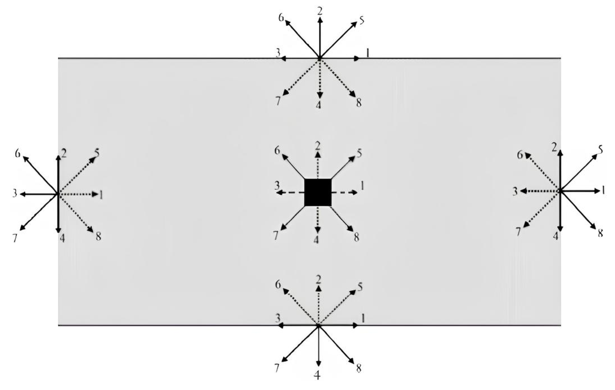
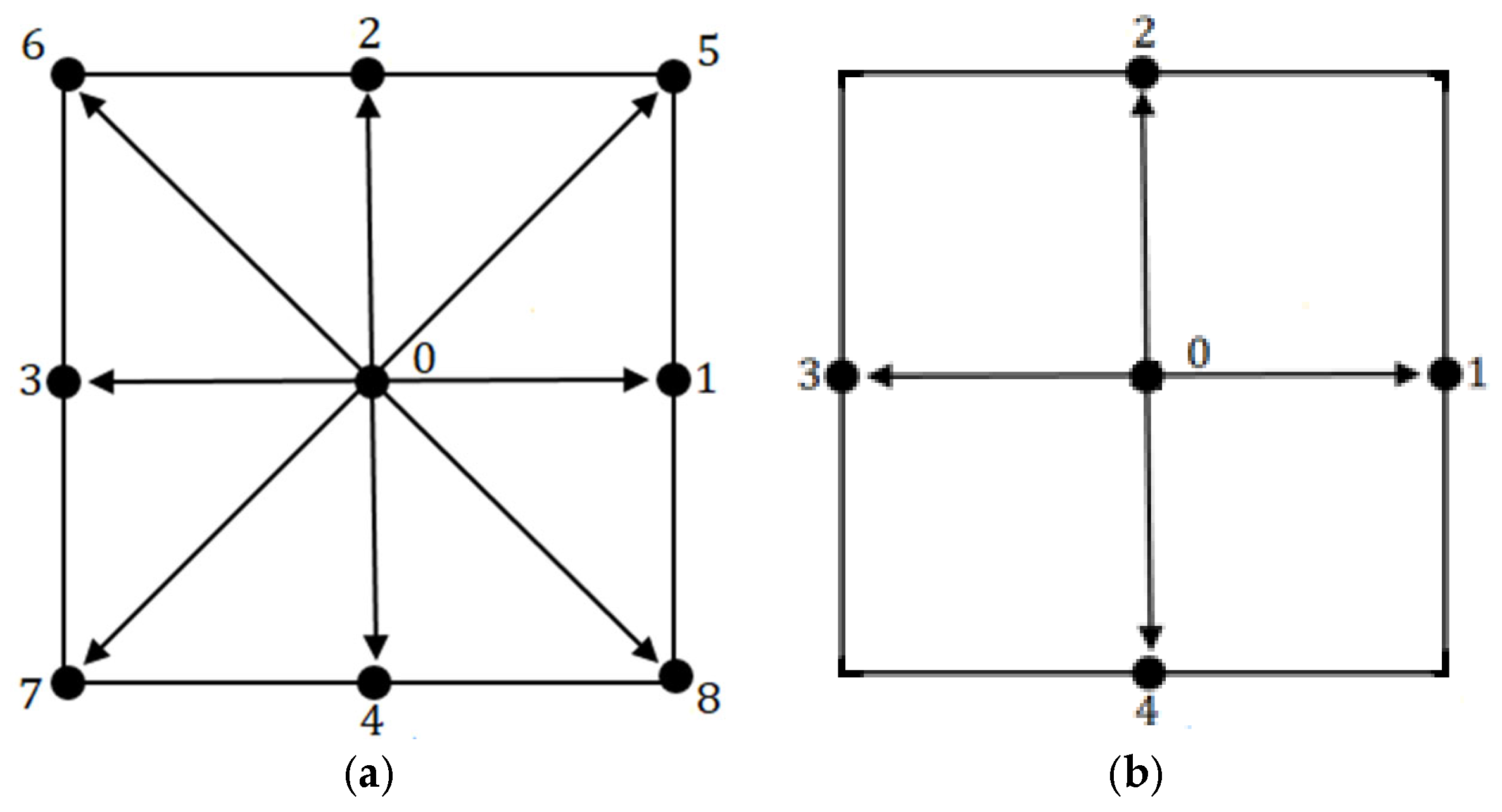
3.1. Lattice Boltzmann Method for Fluid Flow

Figure 3a illustrates the numerical scheme of the $D2Q9$ model used when the particles of fluid move from one node to another adjacent node of the grille with discrete velocities ($c_i$) which are defined by the following:

$$c_i=\left\{\begin{array}{c}\left(\mathrm{0,0}\right); i=0\\ \\ \left(\mathit{cos}\left[{\displaystyle \frac{\left(i-1\right)\pi }{2}}\right],\mathit{sin}\left[{\displaystyle \frac{\left(i-1\right)\pi }{2}}\right]\right)c; i=1–4\\ \\ (\mathit{cos}\left[{\displaystyle \frac{\left(2i-9\right)\pi }{4}}\right],\mathit{sin}\left[{\displaystyle \frac{\left(2i-9\right)\pi }{4}}\right])c; i=5–8\end{array}\right.$$

(12)

The discretization of the lattice Boltzmann equation with the MRT model is expressed by the following:

$$fi\left(x+ci\Delta t,t+\Delta t\right)=fi\left(x,t\right)+\Omega \left(f\right),\hspace{1em}\hspace{1em}i=0,1,\dots .,8$$

(13)

where the $f_i$ and Ω denote, respectively, the particle distribution function and the collision operator developed by D’Humières using the LBM-BGK model [21]. The introduction of this evolution proposed by D’Humières [21] allows us to write the preceding equation as follows:

$$fi\left(x+ci\Delta t,t+1\right)-fi\left(x,t\right)=M^{-1}\times { S}_i\times \left(m_i\left(x,t\right)-{m_i}^{eq}\left(x,t\right)\right),\hspace{1em}\hspace{1em}i=0,\dots ,8$$

(14)

where $M^{-1}$ and $S_i$ represent the inverse matrix of the transformation matrix $M$ and the diagonal relaxation time matrix, respectively. Thus, $m_i$ and ${m_i}^{eq}$ represent, respectively, the momentum vectors and the equilibrium momentum, which are shown as follows:

$$m={(m_0,m_1,m_2,,m_n)}^T ; { m}^{eq}={(\rho ,e^{eq},{\epsilon }^{eq},j_x,q_x^{eq},{j_y,q}_y^{eq},p_{xx}^{eq},p_{xy}^{eq})}^T$$

(15)

The choice of the equilibrium functions $m_i^{eq}$ will determine the equivalent macroscopic equations, which are as follows:

$$\begin{gathered} \begin{array}{l}{m}_0^{eq}=\rho \\ m_1^{eq}=e^{eq}=-2\rho +3(j_x^2+j_y²) \\ {m}_2^{eq}={\epsilon }^{eq}=\rho -3(j_x^2+j_y²)/\rho \\ m_3^{eq}=j_x\\ m_4^{eq}=q_x^{eq}=-j_x\\ m_5^{eq}=j_y\\ m_6^{eq}=q_y^{eq}=-j_y\\ m_7^{eq}=p_{xx}^{eq}=(j_x^2-j_y²)/\rho \\ m_8^{eq}=p_{xy}^{eq}=\left(j_x{j}_y\right)/\rho \end{array} \end{gathered}$$

(16)

where

$$j_x={\rho u}_x={\sum }_i{f}_i^{eq}{C}_{ix}$$

(17)

$$j_y={\rho u}_y={\sum }_i{f}_i^{eq}{C}_{iy}$$

(18)

The expression of the transformation representing the passage from the space of the velocities to the space of the quantities of motions is given by:

$$m=Mf \hspace{1em}\mathrm{and}\hspace{1em} f=M^{-1}m$$

(19)

The matrix M of order 9 is given by [18] and is as follows:

$$\mathrm{M}=\left(\begin{array}{c}〈{\mathit{m}}_0|\\ 〈{\mathit{m}}_1|\\ 〈{\mathit{m}}_2|\\ 〈{\mathit{m}}_3|\\ 〈{\mathit{m}}_4|\\ 〈{\mathit{m}}_5|\\ 〈{\mathit{m}}_6|\\ 〈{\mathit{m}}_7|\\ 〈{\mathit{m}}_8|\end{array}\right)=\left(\begin{array}{cc}\begin{array}{c}1\\ \begin{array}{c}-4\\ \begin{array}{c}4\\ \begin{array}{c}0\\ \begin{array}{c}0\\ \begin{array}{c}0\\ \begin{array}{c}0\\ \begin{array}{c}0\\ 0\end{array}\end{array}\end{array}\end{array}\end{array}\end{array}\end{array}\end{array}& \begin{array}{cc}\begin{array}{c}1\\ \begin{array}{c}-1\\ \begin{array}{c}-2\\ \begin{array}{c}1\\ \begin{array}{c}-2\\ \begin{array}{c}0\\ \begin{array}{c}0\\ \begin{array}{c}1\\ 0\end{array}\end{array}\end{array}\end{array}\end{array}\end{array}\end{array}\end{array}& \begin{array}{cc}\begin{array}{c}1\\ \begin{array}{c}-1\\ \begin{array}{c}-2\\ \begin{array}{c}0\\ \begin{array}{c}0\\ \begin{array}{c}1\\ \begin{array}{c}-2\\ \begin{array}{c}-1\\ 0\end{array}\end{array}\end{array}\end{array}\end{array}\end{array}\end{array}\end{array}& \begin{array}{cc}\begin{array}{c}1\\ \begin{array}{c}-1\\ \begin{array}{c}-2\\ \begin{array}{c}-1\\ \begin{array}{c}2\\ \begin{array}{c}0\\ \begin{array}{c}0\\ \begin{array}{c}1\\ 0\end{array}\end{array}\end{array}\end{array}\end{array}\end{array}\end{array}\end{array}& \begin{array}{cc}\begin{array}{c}1\\ \begin{array}{c}-1\\ \begin{array}{c}-2\\ \begin{array}{c}0\\ \begin{array}{c}0\\ \begin{array}{c}-1\\ \begin{array}{c}2\\ \begin{array}{c}-1\\ 0\end{array}\end{array}\end{array}\end{array}\end{array}\end{array}\end{array}\end{array}& \begin{array}{cc}\begin{array}{c}1\\ \begin{array}{c}2\\ \begin{array}{c}1\\ \begin{array}{c}1\\ \begin{array}{c}1\\ \begin{array}{c}1\\ \begin{array}{c}1\\ \begin{array}{c}0\\ 1\end{array}\end{array}\end{array}\end{array}\end{array}\end{array}\end{array}\end{array}& \begin{array}{cc}\begin{array}{c}1\\ \begin{array}{c}2\\ \begin{array}{c}1\\ \begin{array}{c}-1\\ \begin{array}{c}-1\\ \begin{array}{c}1\\ \begin{array}{c}1\\ \begin{array}{c}0\\ -1\end{array}\end{array}\end{array}\end{array}\end{array}\end{array}\end{array}\end{array}& \begin{array}{cc}\begin{array}{c}1\\ \begin{array}{c}2\\ \begin{array}{c}1\\ \begin{array}{c}-1\\ \begin{array}{c}-1\\ \begin{array}{c}-1\\ \begin{array}{c}-1\\ \begin{array}{c}0\\ 1\end{array}\end{array}\end{array}\end{array}\end{array}\end{array}\end{array}\end{array}& \begin{array}{c}1\\ \begin{array}{c}2\\ \begin{array}{c}1\\ \begin{array}{c}1\\ \begin{array}{c}1\\ \begin{array}{c}-1\\ \begin{array}{c}-1\\ \begin{array}{c}0\\ -1\end{array}\end{array}\end{array}\end{array}\end{array}\end{array}\end{array}\end{array}\end{array}\end{array}\end{array}\end{array}\end{array}\end{array}\end{array}\end{array}\right)$$

(20)

The macroscopic quantities such as density ρ and momentum ρu are determined after the computational process by the following expression [18]:

$$\rho =\sum _{i=0}^8{f}_i,\hspace{1em} \rho u=\sum _{i=0}^8{c}_i{f}_i$$

(21)

3.2. Thermal Lattice Boltzmann Method

For reasons of compatibility (in terms of stability, accuracy, convergence, and calculation time) with the D2Q9 model (Figure 3a), the D2Q5 model was chosen to simulate the temperature field.

Figure 3b illustrates the numerical scheme of the $D2Q5$ model used when the particles of fluid move from one node to another adjacent node of the grille with discrete velocities ($c_i$), which are defined by the following:

$$c_i=\left\{\begin{array}{c}\left(\mathrm{0,0}\right) ; i=0 \\ \\ \left(\mathit{cos}\left[\left(i-1\right){\displaystyle \frac{\pi }{2}})\right], \mathit{sin}\left[\left(i-1\right){\displaystyle \frac{\pi }{2}})\right]\right)c, i=1,\dots , 4\end{array} \right.$$

(22)

The thermal LBE-MRT equation can be formulated, as indicated in the following expression:

$${\mathit{g}}_{\mathit{i}}\left({\mathit{x}+\mathit{e}}_{\mathit{i}}\times ∆\mathit{t},\mathit{t}+∆\mathit{t}\right){-\mathit{g}}_{\mathit{i}}\left(\mathit{x},\mathit{t}\right){=\mathit{N}}^{-1}{\times \mathit{Q}}_{\mathit{i}}\times \left({\mathit{n}}_{\mathit{i}}\left(\mathit{x},\mathit{t}\right)-{{\mathit{n}}_{\mathit{i}}}^{\mathit{e}\mathit{q}}\left(\mathit{x},\mathit{t}\right)\right), \mathbf{i}=0,\dots ,4$$

(23)

where $g_i$ represents the distribution function of the thermal field, $N$ denotes the $5\times 5$ transformation matrix, and $Q$ is the diagonal relaxation time matrix for the thermal problem. Thus, the quantities $n_i$ and ${n_i}^{eq}$ represent, respectively, the thermal momentum and equilibrium thermal momentum in the moment space.

The transformation matrix N is given by [18]:

$$\mathrm{N}=\left(\begin{array}{ccc}\begin{array}{c}1\\ 0\\ \begin{array}{c}0\\ -4\\ 0\end{array}\end{array}& \begin{array}{c}1\\ 1\\ \begin{array}{c}0\\ 1\\ 1\end{array}\end{array}& \begin{array}{ccc}\begin{array}{c}1\\ 0\\ \begin{array}{c}1\\ 1\\ -1\end{array}\end{array}& \begin{array}{c}1\\ -1\\ \begin{array}{c}0\\ 1\\ 1\end{array}\end{array}& \begin{array}{c}1\\ 0\\ \begin{array}{c}-1\\ 1\\ -1\end{array}\end{array}\end{array}\end{array}\right)$$

(24)

The macroscopic quantity calculated in the thermal field after the numerical computation is the temperature, and its expression is given by:

$$\mathrm{T}=\sum _{i=0}^4{g}_i$$

(25)

The LBM algorithm is essentially composed of four subroutines:

❖

Collisions,

❖

Propagation (streaming),

❖

Boundary conditions,

❖

Macroscopic quantities.

The first three subroutines provide updates to the distribution function. The fourth subroutine calculates macroscopic quantities such as the density $\rho$, the fluid velocities ($\overrightarrow{u},\overrightarrow{v}$), and the temperature $T$ which are used in collision calculations.

3.3. Physical Parameters

• Nusselt number

The Nusselt number explains the thermal exchange rate between the cold air and the heated cylinder. The average Nusselt number is calculated by the following expression:

$$N_u={-d\times \left({\displaystyle \frac{\partial \theta }{\partial n}}\right)}_{Surface}$$

(26)

where $\mathrm{“}n\mathrm{”}$ and $\mathrm{“}d\mathrm{”}$ represent the normal and the face length of the cylinder, respectively.

The space-average Nusselt number around a square obstacle is defined by the following:

$$\{\begin{array}{}\mathrm{(27)}& {Nu}_i={\int }_0^{d/H}-d\times {\displaystyle \frac{\partial \theta }{\partial X}}.dY \mathrm{F}\mathrm{o}\mathrm{r} \mathrm{t}\mathrm{r}\mathrm{a}\mathrm{n}\mathrm{s}\mathrm{v}\mathrm{e}\mathrm{r}\mathrm{s}\mathrm{e} \mathrm{f}\mathrm{a}\mathrm{c}\mathrm{e}\mathrm{s}\mathrm{(28)}& {Nu}_i={\int }_0^{d/H}-d\times {\displaystyle \frac{\partial \theta }{\partial Y}}.dX \mathrm{F}\mathrm{o}\mathrm{r} \mathrm{h}\mathrm{o}\mathrm{r}\mathrm{i}\mathrm{z}\mathrm{o}\mathrm{n}\mathrm{t}\mathrm{a}\mathrm{l}\mathrm{e} \mathrm{f}\mathrm{a}\mathrm{c}\mathrm{e}\mathrm{s} \end{array}$$

• Drag coefficient

The drag coefficient, often referred to as $Cd$, is a dimensionless quantity that characterizes the resistance experienced by an object moving in a fluid (in this study, air). It is used to quantify the drag force acting on the object and is an essential parameter in the study of fluid dynamics and aerodynamics. It plays a crucial role in understanding and designing various technical applications. The drag coefficient $Cd$ is computed by integrating the pressure and shear stress distributions over the surface of the rectangular cylinder. It is defined as follows:

$$Cd={\displaystyle \frac{2\times F_D}{\rho .U_{Ref}^2.D}}$$

(29)

where

${\mathit{F}}_{\mathit{D}}$ is the total drag force acting on the obstacle,

ρ is the fluid density,

Uref is the reference velocity (usually the inlet or the maximal velocity),

$\mathit{D}$ is the characteristic surface area of the obstacle (typically its frontal area).

In the lattice Boltzmann method (LBM), the drag force is determined by summing the momentum exchange between fluid particles at the solid boundary. Using the momentum exchange method, the local force at each node of the boundary is given by the following:

$$\sum {\mathit{f}}_{\mathit{i}}{\mathit{e}}_{\mathit{i}}.$$

where ${\mathit{f}}_{\mathit{i}}$ represents the post-collision distribution function, and ${\mathit{e}}_{\mathit{i}}$ is the discrete velocity vector. The total drag force is obtained by integrating this force over all boundary nodes of the obstacle.

• Reynolds number

The Reynolds number is an essential non-dimensional number in the study of air dynamics. This number characterizes the fluid flow regime and is defined by the following:

$$Re={\displaystyle \frac{U_{max}\times D}{\upsilon }}$$

(30)

Boundary conditions significantly affect the accuracy of both the computed drag coefficient ($Cd$) and the Nusselt number ($Nu$), particularly in confined flows. The key boundary conditions used in this study and their influence on these parameters are discussed in the boundary conditions section. Indeed, the accurate prediction of the drag coefficient and the Nusselt number requires careful implementation of the boundary conditions, especially in confined flows. The choice of inlet velocity profile, outlet treatment, and wall constraints significantly impacts the flow dynamics and consequently the computed values of Cd, which influences the Nusselt number distribution across the obstacle faces. The proper selection and implementation of these boundary conditions are crucial for obtaining reliable results in both aerodynamic and thermal performance analyses. In this study, the drag coefficient and the Nusselt number results are validated against the existing literature to ensure reliability.

The application of the LBM to real problems requires an appropriate conversion from the mesoscopic scale (lattice units) to physical scale (conventional units) and vice versa. For this reason, we have included a conversion appendix at the end of the manuscript (See Appendix A).

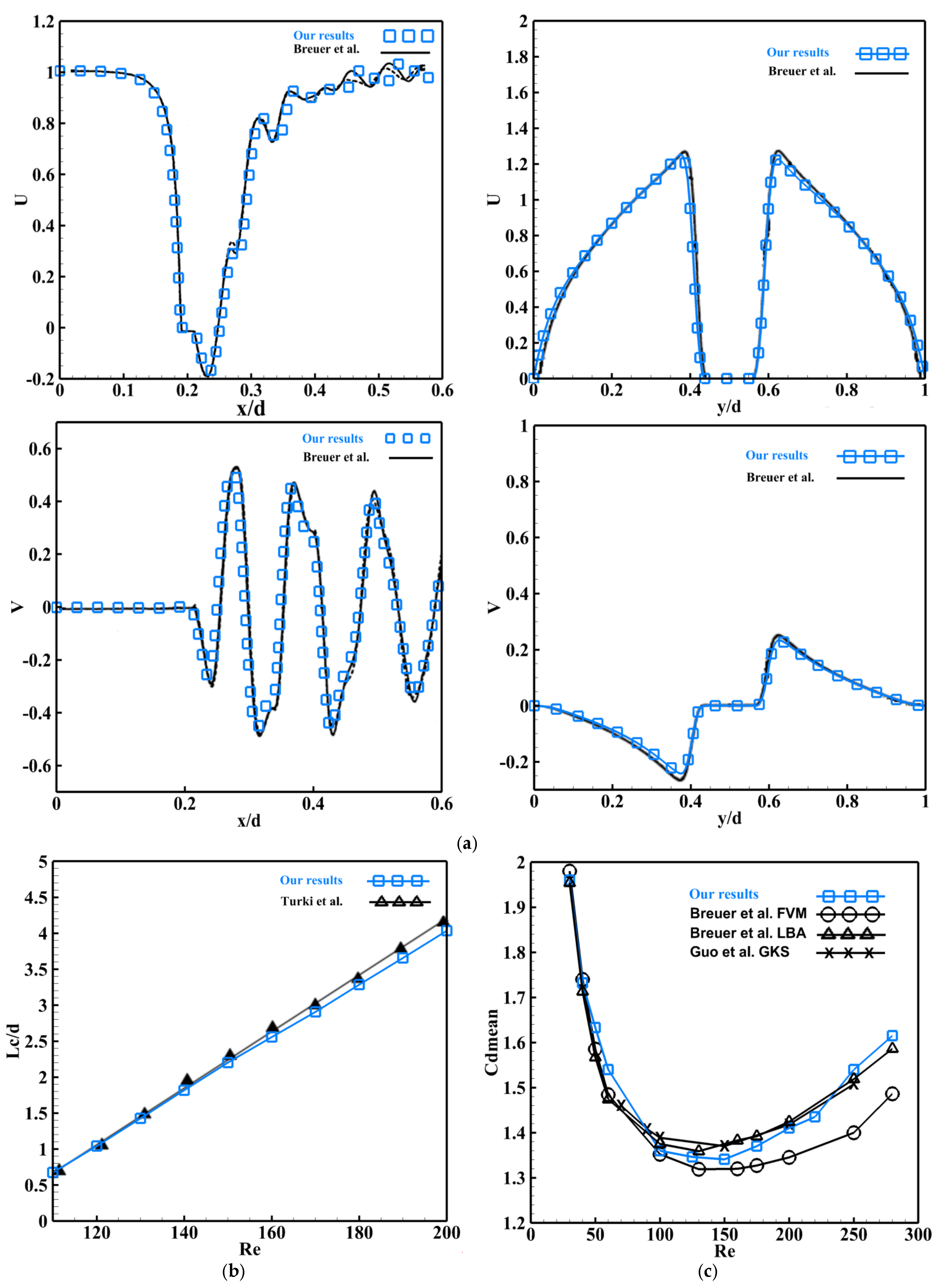
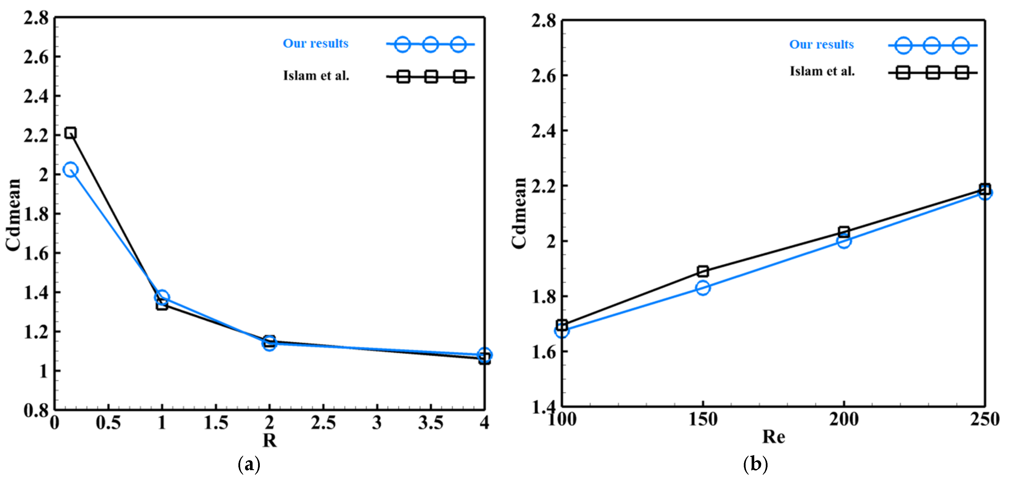
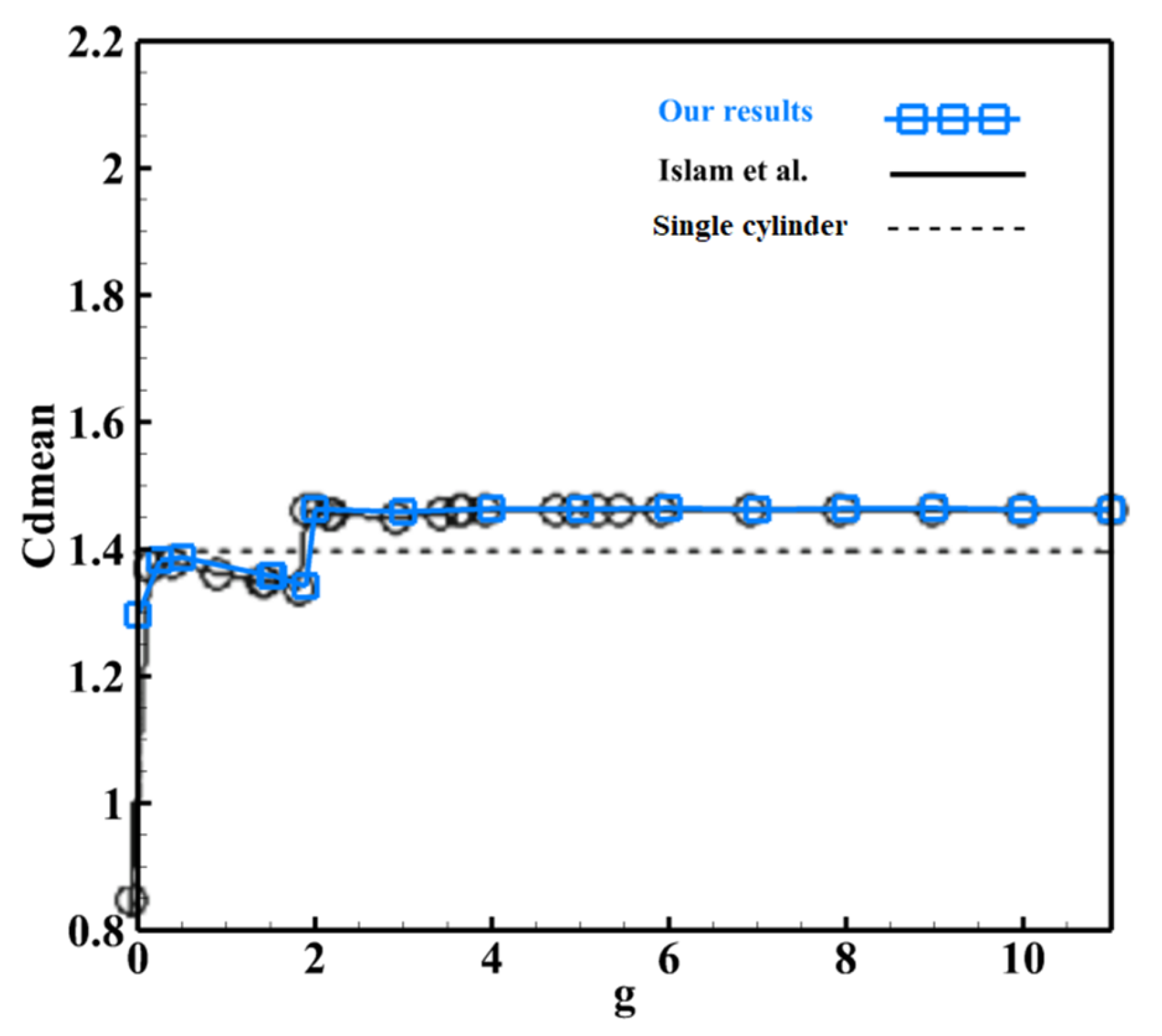
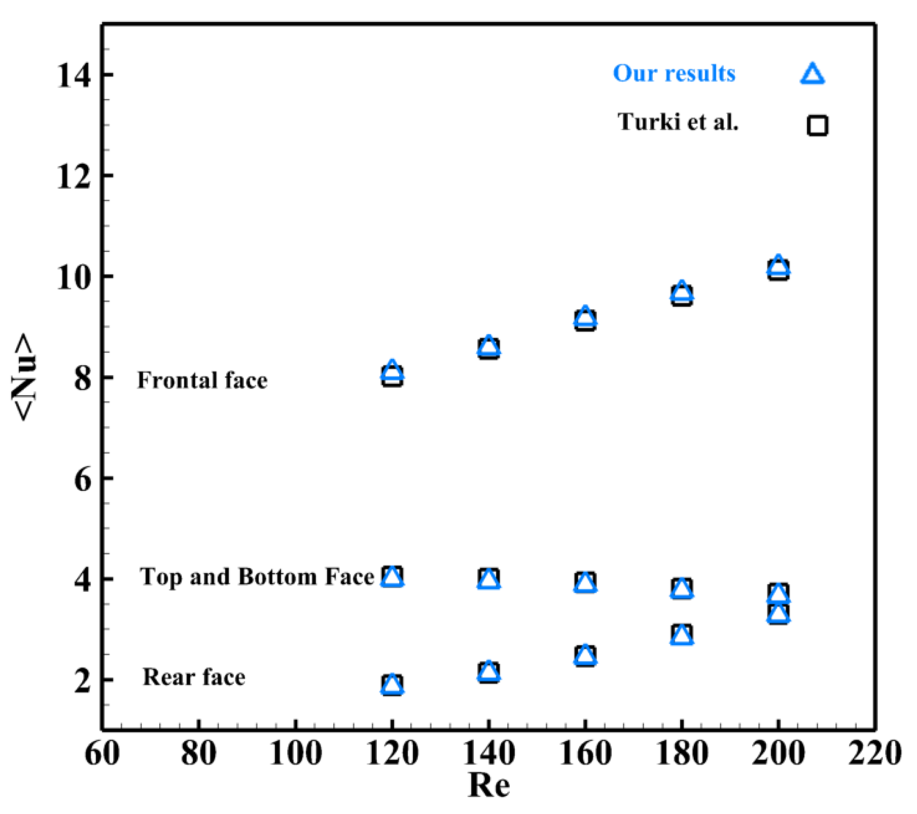
4. Validation of Numerical Code

The first validation case focuses on airflow around a square obstacle. This problem was previously investigated by Breuer et al. [28] using the lattice Boltzmann method with the single relaxation time model (LBM-SRT) and the finite volume method (FVM). Guo et al. [29] then reused this configuration for a comparison between the lattice Boltzmann method with multiple relaxation times and the gas kinetics scheme (GKS).

Figure 4a–c show, respectively, the velocity profiles along the x and y axes, the variation in the recirculation length behind the square obstacle as a function of the Reynolds number, and the variation in the average drag coefficient for different values of the Reynolds number varying between $5$ and $300$. It should be noted that the finite volume and lattice Boltzmann methods used by Breuer et al. [28] are applied to non-uniform ($560\times 340$) and uniform ($2000\times 320$) grids, respectively, whereas the results of Guo et al. [29] are obtained using the gas kinetics scheme (GKS) with a ($1001\times 161$) grid.

The comparison of the results demonstrates a slight discrepancy (below 1.7%) relative to the numerical findings of Breuer et al. [28], Guo et al. [29] and Turki et al. [9]. This difference is generally due to the grid used. Indeed, the length of the recirculations formed behind the obstacle increases with increasing Reynolds numbers. The average values of the drag coefficient exhibit a decreasing trend with increasing Reynolds numbers until reaching a minimum, after which a subsequent increase is observed. This is due to the fact that for low Reynolds numbers, viscosity effects are more intense than inertia effects. As the Reynolds number increases, so does the velocity of the fluid particles. Consequently, the generation of vortices behind the obstacle increases. As a result, the average values of the drag coefficient increase.

Given that the present study involves both a rectangular cylinder and a control partition, a second validation analysis is conducted. This validation focuses on the flow around a rectangular cylinder without a control plate, with a blockage ratio of $\beta =1/8$, across a Reynolds number range of $100 \le Re \le 250$. The numerical results are compared with those obtained by Islam et al. [30] to assess the accuracy of our approach. Two validation graphs are presented. Figure 5a illustrates the variation in the mean drag coefficient ${Cd}_{mean}$ as a function of the aspect ratio $R=width/height$. The results indicate that ${Cd}_{mean}$ decreases as the aspect ratio increases, aligning closely with the reference data. Figure 5b depicts the evolution of ${Cd}_{mean}$ with respect to the Reynolds number, showing a linear increase in drag as Re rises. Once again, our findings demonstrate strong agreement with those reported by Islam et al. [30], reinforcing the reliability of the numerical methodology employed in this work.

A further validation study was added to ensure the quality and precision of our numerical code. In this investigation, the simulation of the flow of a fluid around a square cylinder controlled by an inclined partition at a blocking ratio $\beta ={\displaystyle \frac{H}{d}}=11$ was performed and validated with the results found by Islam [8]. Figure 6 presents the variation in the average drag coefficient as a function of the distance separating the square obstacle and the control partition at a fixed Reynolds number ($Re=150$).

The graphical analysis confirms strong agreement between the results, which can be attributed to the consistent use of the same numerical approach, specifically the LBM-MRT model.

To validate the accuracy of the present numerical code for the thermal problem, a comparative study was conducted by analyzing the Nusselt number against reference data from the literature [31]. As shown in

Table 1. Average Nusselt number validation and maximum deviation for each face of a square cylinder.

Source (Frontal Face)	$\mathit{R}\mathit{e}=25$		$\mathit{R}\mathit{e}=30$		$\mathit{R}\mathit{e}=35$		$\mathit{R}\mathit{e}=40$		$\mathit{R}\mathit{e}=45$
	$\mathit{N}\mathit{u}$	%	$\mathit{N}\mathit{u}$	%	$\mathit{N}\mathit{u}$	%	$\mathit{N}\mathit{u}$	%	Nu	%
Our results	3.55 0.84% 3.58		3.88 0.78% 3.85		4.19 0.47% 4.21		4.48 1.10% 4.53		4.76 0.21% 4.75
Dhiman et al. [31]
Source (Top or Bottom face)	$Re=25$		$Re=30$		$Re=35$		$Re=40$		$Re=45$
	$Nu$	%	$Nu$	%	$Nu$	%	$Nu$	%	$Nu$	%
Our results	0.91 0.011% 0.90		0.93 2.197% 0.91		0.96 1.05% 0.95		0.986 0.61% 0.98		1.019 0.098% 1.02
Dhiman et al. [31]
Source (Rear face)	$Re=25$		$Re=30$		$Re=35$		$Re=40$		$Re=45$
	$Nu$	%	$Nu$	%	$Nu$	%	$Nu$	%	$Nu$	%
Our results	2.27 1.33% 2.24		2.37 0.85% 2.35		2.45 0.4% 2.46		2.52 1.94% 2.57		2.58 1.9% 2.63
Dhiman et al. [31]

, the average Nusselt number was evaluated for each face of the cylinder, with a particular focus on the maximum deviation at a low Reynolds number. The results demonstrate strong agreement with the reference values reported in [31], confirming the reliability of the numerical approach.

Likewise, Turki et al. [9] treated the flow of air associated with the convective heat transfer around a square obstacle which is heated and inserted inside a horizontal channel. These authors used the finite volume method (FVM) with non-uniform meshes of $(122\times 57)$ and $(122\times 77)$, respectively, for blocking ratios at $\beta =1/4$ and $\beta =1/8$.

Figure 7 illustrates the mean Nusselt number variations as a function of the Reynolds number on all faces of the obstacle. The current results are compared with those obtained by Turki et al. [9]. The heat exchange between the fluid and the front face is observed to be more pronounced than that occurring on the other faces. This is due to the direct contact between the fluid particles and this face, whereas this exchange decreases strongly on the rear face due to the recirculations formed behind this face. Also, the following graph illustrates that the obtained results are similar to those of Turki et al. [9].

Figure 8 illustrates the stability and rapid convergence of our numerical code, highlighting the effectiveness of the adopted approximations. These results confirm that the LBM-MRT-based approach is well suited for the accurate simulation of fluid flow and heat transfer phenomena. It ensures both reliability and computational efficiency.

5. Results and Discussion

The numerical results for the flow around a rectangular cylinder influenced by an inclined partition are presented in this section. The study examines the effect of the Reynolds number and the distance between the partition and the rectangular block. The results are analyzed through visualizations of thermal vortex shedding patterns, the drag coefficient temporal evolution, and the averaged Nusselt number variations.

5.1. Reynolds Number Effect

Figure 9 presents an analysis of thermal vortex shedding over a Reynolds number range from $100$to $250$. In this case, the control partition length remains fixed at $Lp=1d$, while the position is set at $g=1d$. The results reveal the presence of three different flow regimes, each characterized by unique dynamics. Initially, at a $Re=100$ (Figure 9a), the flow regime exhibits periodicity with subtle undulations. When the $Re$is increased to 150 (Figure 9b), the periodicity persists, but with slightly more pronounced undulations. However, as the $Re$increases to values between $200$ and 250 (Figure 9c,d), the flow regime enters a more turbulent phase marked by significant undulations.

Indeed, when the Reynolds number increases, it generally means that the velocity of the fluid particles increases in relation to the viscosity of the fluid. This increase in the velocity can have significant effects on the flow dynamics and heat exchange. In the context of ripple formation in a flow, an increase in the Reynolds number translates into an increase in the vortex strength and pressure fluctuations generated by the flow. As a result, the ripples become more pronounced and irregular. This intensification of ripple amplitude is often associated with an increase in flow turbulence, meaning that velocity and pressure fluctuations become more chaotic and less predictable. Likewise, as vortex shedding increases, the flow will have a more homogeneous temperature distribution. As a result, temperature gradients become more pronounced. This increase in temperature gradients can be observed at different levels of the flow, notably near obstacle surfaces and in recirculation zones behind the obstacle.

In particular, the areas where vortexes form and dissipate may exhibit steeper temperature gradients due to increased mixing between the cold fluid and the hot obstacle. These temperature gradients can be amplified by eddy-induced turbulence, as local variations in velocity and pressure can also lead to temperature variations. In addition, vortexes can influence thermal convection by altering flow patterns around the obstacle, which in turn can modify heat transfer rates to obstacle surfaces. This leads to a significant increase in the overall heat exchange between the obstacle and the surrounding fluid.

At the same time, the increase in turbulence also increases the amplitude of the periodicity of the flow; as the fluctuations become more pronounced, the amplitude of the Von Karmann street of the flow increases.

5.1.1. Variation in the Drag Coefficient for $100\le Re\le 250$

The influence of the Reynolds number on the temporal evolution of the drag coefficient is a key focus of this study, as it provides valuable insights into the aerodynamic behavior of the flow. Figure 10 illustrates this variation for a range of Reynolds numbers from $Re=100$ to $Re=250$. An important observation is the regularity and periodicity of the evolution of the drag coefficient over this Reynolds range. However, a notable difference lies in the amplitude of the drag coefficient for the Reynolds sub-ranges. In particular, for the sub-range of $200 \le Re \le 250$ the amplitude of the drag coefficient is larger than for $100 \le Re \le 150$. This difference in amplitude can be attributed to the direct effect of increasing the Reynolds number on the flow dynamics. Increasing the Reynolds number leads the fluid to flow faster around the obstacle. This increase in fluid velocity leads to a more intense interaction between the fluid and the obstacle, particularly with the presence of the inclined partition. The fluid–structure interaction modifies and disrupts the flow patterns and leads to a redistribution of the shear layers generated by the partition borders. These shear layers are then advected downstream and affect the flow behavior around the rectangular block faces. This redistribution creates zones of high and low pressure on the surfaces of the obstacle. This pressure gradient generates thrust forces on the obstacle surfaces. As a result, pressure fluctuations generate negative drag force values, as depicted in the figure. Notably, this phenomenon leads to a substantial reduction in the mean drag coefficient (${Cd}_{mean}$), highlighting the impact of flow control on aerodynamic performance, reaching a maximum percentage reduction of $125.41\%$ for $Re=250$. This substantial reduction in the drag force illustrates the significant impact of the increase in the Reynolds number on the flow dynamics and its effects on the fluidic forces exerted on the obstacle.

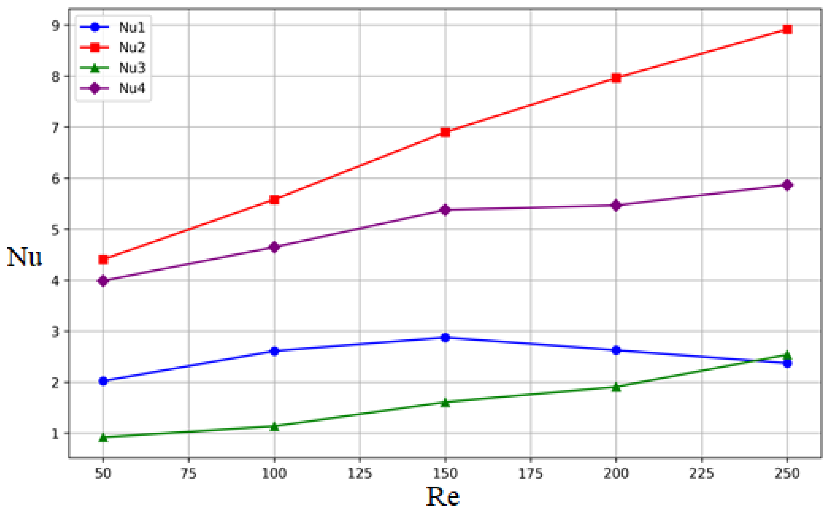
5.1.2. Nusselt Number Variation for $100\le Re\le 250$

In thermal systems, the efficiency of heat transfer plays a crucial role in optimizing energy performance. The integration of an inclined control partition in internal flow configurations, such as the channel containing a rectangular cylinder, represents a promising passive strategy to improve these transfers. In this section, the variation in the average Nusselt number is examined for each face of the obstacle at the various Reynolds numbers $100 \le Re \le 250$. This variation has been studied for a fixed gap spacing ($g=1d$).

The graphs in Figure 11 illustrate the variation in the average Nusselt number $Nu$ for different faces of a rectangular cylinder as a function of the Reynolds number $Re$. The graphs corresponding to ${Nu}_1$, ${Nu}_2$, ${Nu}_3$, and ${Nu}_4$ represent the variation in the mean Nusselt number on the front, top, rear, and bottom faces of the cylinder, respectively. A distinct evolution of $Nu$ for each face with increasing Re was observed. The behavior of the graphs highlights the variation in heat exchange, measured by $Nu$, on each face of the cylinder due to flow effects, measured by $Re$, and by the control partition. These results clearly illustrate the impact of the inclined partition on the variation in the average Nusselt number $Nu$ as a function of the Reynolds number $Re$, as well as the specific characteristics of the heat transfers on the different faces of the rectangular cylinder.

The fluid directly impacts the front face (${Nu}_1$). Its evolution is characterized by an initial increase between $Re=50$ and e, a trend which is explained by the combined effect of the flow regime and the disturbances induced by the boundary layer separation. At low $Re$, the flow remains predominantly laminar, favoring efficient heat exchange. However, at higher $Re$ ($Re>150$), boundary layer separation and the formation of vortex structures reduce heat transfer efficiency, leading to a progressive reduction in ${Nu}_1$. In contrast to ${Nu}_1$, ${Nu}_2$ (top face) increases monotonically with Re, reaching a maximum at $Re=250$. This increase is explained by the intensification of shear layers and the formation of vortex structures favoring better heat exchange. The inclination of the partition plays an essential role here, directing and concentrating the flow on this face. The thermal improvement is particularly marked, reaching $82.87\%$ at $Re=250$, demonstrating a clear optimization of heat transfer with increasing Re. Whereas, the evolution of ${Nu}_{3 }$ (rear face) shows a gradual increase, most marked from $Re\ge 150$. The recirculation zone behind the cylinder is limited at low $Re$, which restricts heat transfer. From $Re=150$ onwards, the development of recirculation zones and the presence of vortices behind the cylinder promotes increased thermal mixing, improving ${Nu}_3$. However, at higher $Re$ numbers, this improvement is partially offset by the interaction effects between vortex structures and the loss of thermal mixing efficiency. A decrease of $-28.24\%$ is observed at $Re=250$, indicating some degradation of heat transfer in this zone. For the lower face, the graph illustrating ${Nu}_4$shows a steady increase with Re, albeit slightly lower than for ${Nu}_2.$ This relative similarity between ${Nu}_2$ and ${Nu}_4$can be explained by the symmetry of the flow in the channel. However, the upper face benefits from more intense shear induced by the inclination of the partition, giving it a thermal advantage. The thermal improvement reaches $30.67\%$ at $Re=250$, reflecting the significant influence of an increasing $Re$ on heat transfer to this face.

The addition of an inclined partition is an effective method of maximizing heat transfer on certain cylinder surfaces. These results are particularly promising for practical applications, such as the cooling of electronic components or the improvement of heat transfer systems in thermal and aeronautic engineering. Further optimization of the angle of inclination and position of the partition could further improve overall performance, in particular by reducing heat transfer deterioration on the front and rear faces.

5.2. Gap Spacing Effect

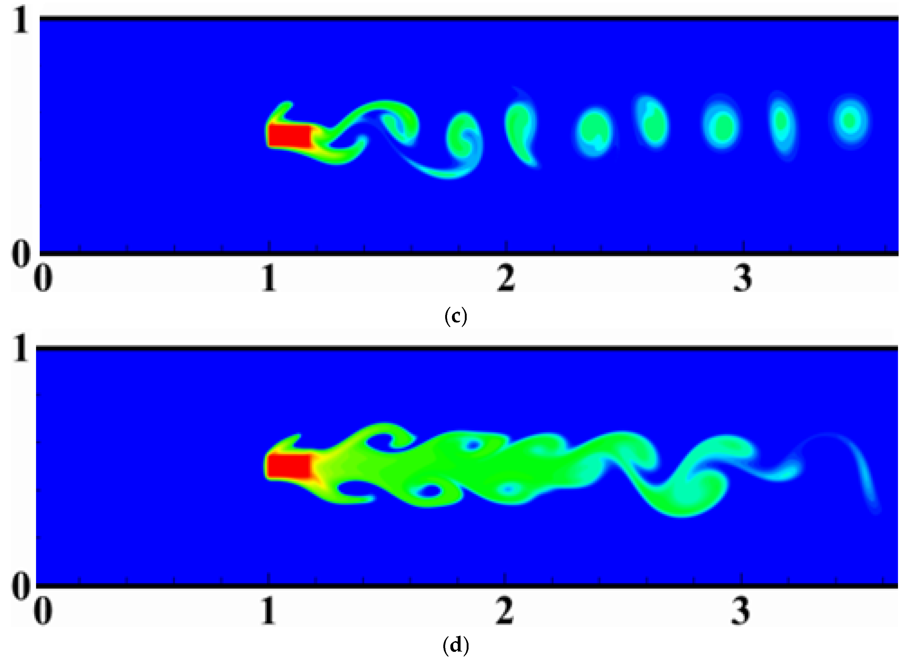
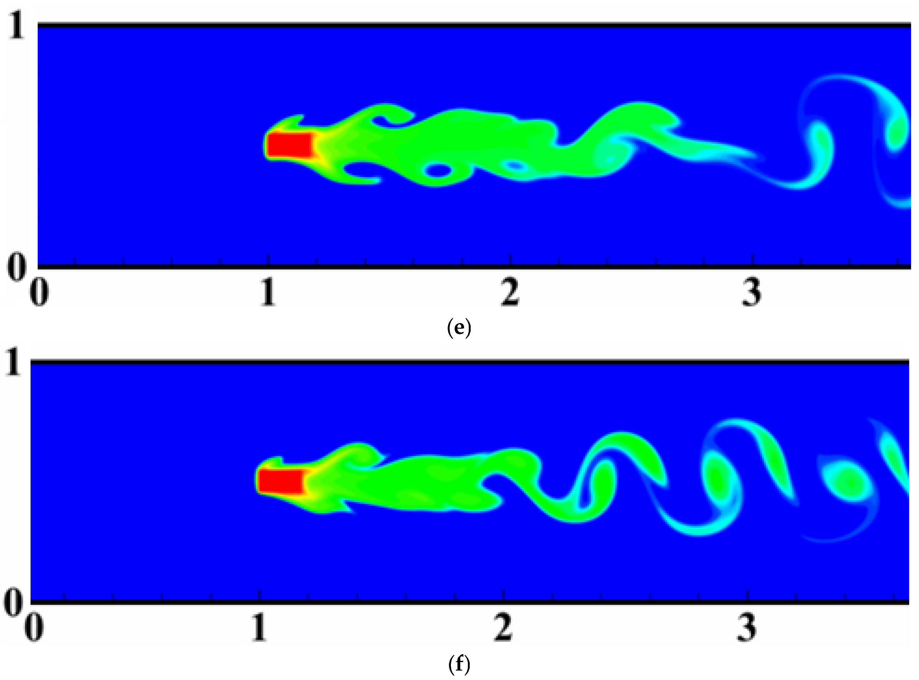
5.2.1. Influence of a Spacing Gap on Thermal Vortex Shedding

The impact of the position of the control partition relative to the rectangular cylinder on thermal vortex shedding is analyzed in this section. The Reynolds number is held constant at $Re=150$, while the length of the control partition is fixed at $Lp=1d.$ Figure 12 provides a thermal vortex visualization around and downstream of the cylinder for different gap spacings. The results show three distinct thermal regimes, each with unique heat transfer characteristics. For a small gap spacing (Figure 12a,b), the moving fluid perceives the partition and the rectangular cylinder as a single obstacle. In this configuration, the shear layers bypass the obstacle, resulting in periodic vortex shedding behind it. Nevertheless, as the gap g increases, both the number and shape of the vortices increase until they become almost imperceptible (Figure 12c–e). This occurs because the shear layers generated by the partition directly impact the block and its wake, inducing significant recirculation zones behind the cylinder. This alteration in heat flow results in an irregular thermal regime. When the space between the bulkhead and the cylinder becomes very large (Figure 12f,g), the fluidic shear layers fall into the space between the two bodies and interact with the cylinder in the same way as in an uncontrolled scenario. In the last case, the thermal vortex shedding exhibits an alternating pattern of positive and negative vortices, characteristic of classical vortex shedding.

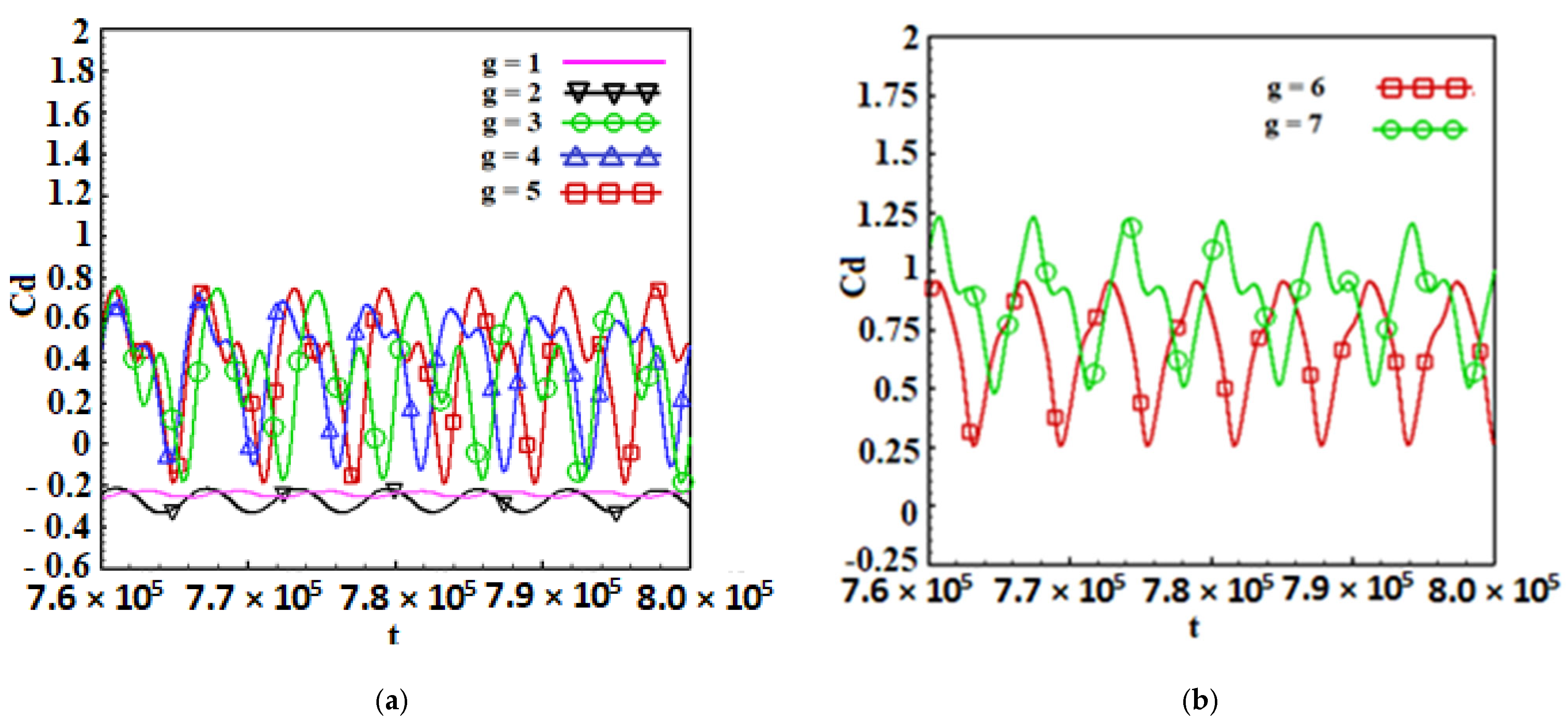
5.2.2. Drag Coefficient Variation for $1d\le g\le 8d$ at $Re=150$

The effect of the relative positioning between the inclined plate and the rectangular cylinder on the temporal evolution of the drag coefficient (Cd) is examined at a fixed Reynolds number ($Re=150$). Figure 13 illustrates the temporal curves of $Cd$ for different gap distances g between the control plate and the cylinder.

As shown in Figure 13a, when the gap spacing is small ($g=1d-2d$) the amplitude of the drag coefficient oscillations is significantly reduced. In this configuration, the inclined plate acts as a stabilizing element, attenuating fluctuations in $Cd$, leading to a $130.97\%$ reduction in the mean drag coefficient compared to the case without the control plate, where the mean drag coefficient is ${Cd}_{mean}=1.13$. This optimal reduction in $Cd$ translates into a significant decrease in energy losses, thereby improving the aerodynamic efficiency of the system. However, beyond this spacing range, a gradual increase in the temporal values of the drag coefficient is observed. Indeed, as the distance between the inclined plate and the cylinder increases, part of the shear layers manages to escape into the intermediate gap. This phenomenon enhances fluid–structure interactions, resulting in an increase in the forces acting on the cylinder. Consequently, a notable rise in both the mean and instantaneous values of the drag coefficient is observed, indicating that the stabilizing effect of the control plate diminishes as the gap increases.

This study thus highlights the existence of an optimal gap spacing g that minimizes drag and stabilizes the flow. When g is too small, the partition and the cylinder are perceived as a single obstacle, reducing $Cd$ oscillations. Conversely, when g becomes too large, interactions between the structures intensify, leading to higher drag and a more unstable flow.

Having studied the effect of Reynolds number $Re$ variation on thermal performance and aerodynamic behavior, the analysis now focuses on the impact of the upstream spacing g between the control partition and the rectangular cylinder (Figure 14, Figure 15 and Figure 16). This study aims to assess how this distance influences the average Nusselt number $Nu$ for each face of the cylinder (${Nu}_1$,${Nu}_2$,${Nu}_3$,${Nu}_4$) and to identify the optimal conditions for maximizing heat exchange. Various Reynolds numbers ($Re=100, Re=150$, and $Re=200$) are considered in order to study the interaction between flow dynamics and heat transfer as a function of the partition position. This analysis will not only lead to a better understanding of the effect of g on the heat flux distribution but also guide practical applications in areas such as electronic component cooling and thermal management in complex systems.

❖

For $Re=100$

Figure 14 illustrates the variation in the average Nusselt number $Nu$ for the four faces of a rectangular cylinder (${Nu}_1$: front face, ${Nu}_2$: top face, ${Nu}_3$: rear face, ${Nu}_4$: face bottom) as a function of the upstream spacing $g$ between the inclined control partition and the rectangular cylinder. The values of $g$ range from $1d$to $6d$, while $Wc$ corresponds to the case without control partition.

-

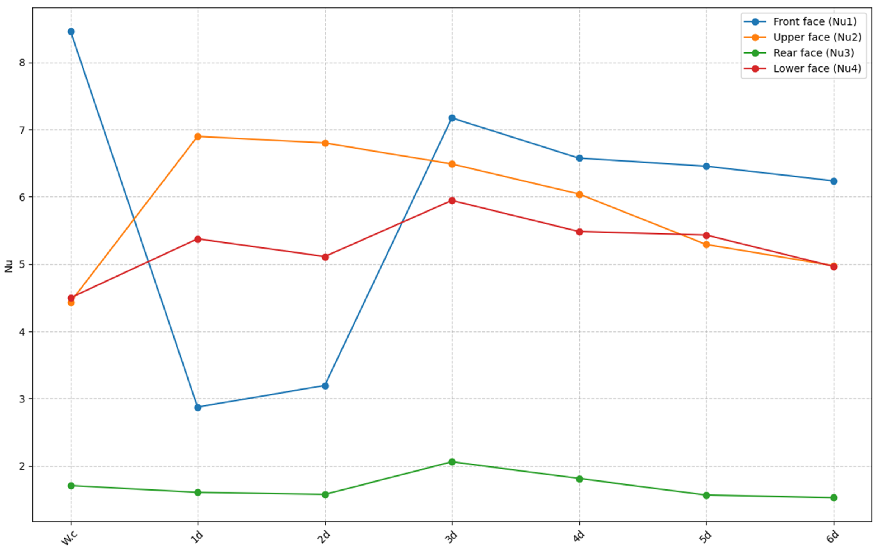
For the front face: The graph representing ${Nu}_1$ shows a maximum value of ${Nu}_1$ for the Wc case. In the presence of the partition, ${Nu}_1$drops drastically for $g=1d$, remains low for $g=2d$ and 3d, before increasing slightly for $g\ge 4d$.

-

For the upper face: The graph representing ${Nu}_2$ shows a clear improvement compared to the Wc case. ${Nu}_2$ increases progressively with g, reaching a maximum at $g=4d$, then decreases slightly for $g=6d$.

-

For the rear face: The graph representing ${Nu}_3$ shows low and stable values, with a slight increase in ${Nu}_3$as g increases.

-

For the bottom face: The graph representing ${Nu}_4$ shows a significant increase compared to the Wc case. ${Nu}_4$ progresses with g, reaching a maximum at $g=4d$ before stabilizing for higher spacings.

Analysis of the results highlights the beneficial effect of the partition position (gap spacing g) on the heat transfer around the rectangular cylinder. Percentage improvements are calculated by comparing each case $(g=1d$ to $6d$) to the reference case Wc.

Front face (${Nu}_1$): In the Wc case, ${Nu}_1$ reaches its maximum value (around $7$). Inserting the partition strongly decreases ${Nu}_1$, especially for $g=1d$. This decrease can be explained by the deviation of the main flow upstream, thus reducing the direct impact of the fluid on the front face. Although ${Nu}_1$ shows a slight improvement for $g=4d$, it remains systematically lower than the case without the partition, reflecting a redistribution of heat transfer to other faces.

Top side (${Nu}_2$): The partition improves ${Nu}_2$ considerably. Compared to Wc, a maximum increase of $27.87\%$ is observed for $g=4d$ thanks to the intensification of shears and vortices on this face. This case ($g=4d$) is considered critical for all cylinder faces. These results show that this placement of the partition favors heat transfer on the upper face, where flow-induced shear is most intense.

Rear face (${Nu}_3$): ${Nu}_3$shows a progressive increase with g. For $g=4d$, an improvement of 14.28% is observed compared to Wc. This improvement is attributed to the development of recirculation zones and vortex structures behind the cylinder, which promote intense thermal mixing. For $g\ge 4d$, ${Nu}_3$ stabilizes, reflecting a saturation of recirculation effects.

Bottom side (${Nu}_4$): ${Nu}_4$ values remain low relative to other faces for low g3d spacings, but a significant increase is observed at $g=4d$. For $g=4d$, ${Nu}_4$ shows a $37\%$ improvement over Wc. This can be explained by an indirect effect of the bulkhead, which strongly disturbs the flow under the cylinder that generates significant shear.

In general, the results show that the inclined partition provides an overall improvement in heat transfer, particularly on the top (${Nu}_2$), rear (${Nu}_3$), and bottom (${Nu}_4$) faces. These improvements reach 27.87%, 14.28%, and 37%, respectively, for $g=4d$, confirming the importance of optimum spacing between the partition and the cylinder. However, the systematic reduction in ${Nu}_1$ highlights a compromise in the redistribution of heat flows. Optimizing the position and inclination of the partition could maximize thermal performance on all sides, opening up the prospects for industrial applications requiring the passive control of heat exchange.

❖

For $Re=150$

The graph in Figure 15 represents the variation in the average Nusselt number $Nu$ for the four faces of a rectangular cylinder (front, top, rear, and bottom) as a function of the upstream spacing g for a Reynolds number fixed at $Re=150$. The different curves are distinguished by specific colors: blue for the front face (${Nu}_1$), orange for the top face (${Nu}_2$), green for the rear face (${Nu}_3$), and red for the bottom face (${Nu}_4$). The Wc case, where the control partition is absent, is also included as a reference. Significant variations in the Nusselt number (Nu) are observed across the different faces of the cylinder for varying values of gap spacing (g). The front face (${Nu}_1$) shows marked variations with a decreasing trend and then a slight increase for g values ranging from $1d$ to $6d$. The top face (${Nu}_2$) peaks at $g=2d$ before gradually decreasing. The rear face (${Nu}_3$) maintains low, relatively stable values. The bottom face (${Nu}_4$) shows a similar behavior to ${Nu}_2$, but with slightly lower values.

Introducing the partition significantly modifies the heat exchange around the cylinder. In the absence of the partition ($Wc$), the front face (${Nu}_1$) reaches a maximum value of around $8$ as it is directly exposed to the airflow without prior disturbance. When the partition is introduced, the marked reduction in ${Nu}_1$ for $g=1d$ reflects a weakening of heat exchange due to the thermal shadow effect created by the partition. However, from $g=3d$ a gradual recovery is observed, suggesting a partial restoration of convective flow on this face. Nevertheless, ${Nu}_1$ remains $15.27\%$ lower than in the case without the partition, indicating a persistent disruption in heat transfer. For the top face (${Nu}_2$), a significant peak is observed at $g=2d$, driven by an intense interaction between the airflow deflected by the partition and the upper cylinder wall. At $g=3d$, heat transfer is notably enhanced, with ${Nu}_2$ increasing by $46.29\%$, indicating a strong effect of vortex-induced convection. However, as g increases further ($g\ge 4d$), a progressive decay is observed, highlighting the diminishing influence of the partition with distance. The rear face (${Nu}_3$) maintains consistently low values, reflecting a wake flow regime that is generally unfavorable for heat exchange. However, at $g=3d$, an improvement of $20.59\%$ is recorded, likely due to modifications in the wake vortex structures that enhance local convection. Likewise, the bottom face (${Nu}_4$) follows a pattern comparable to the top face, but with slightly lower values. At $g=3d$, an improvement of $32.16\%$ is observed, suggesting that the deflected airflow effectively enhances heat transfer on this surface. This enhancement can be attributed to better convective interaction between the airflow and the lower wall of the cylinder.

The spacing g plays an essential role in modulating the heat transfer at a fixed Reynolds number ($Re=150$). When the inclined partition is positioned too close to the cylinder ($g=1d$), it leads to a significant reduction in thermal performance on the front face. In contrast, an intermediate spacing $g=3d$ (critical spacing) enhances heat transfer on the upper and lower faces. For larger distances ($g\ge 4d$), the influence of the partition gradually diminishes, bringing thermal performance near to levels close to those observed in the absence of the control (Wc).

❖

For $Re=200$

The graph in Figure 16 illustrates the evolution of the average Nusselt number $Nu$ for each face of the rectangular cylinder (front, top, rear, and bottom) as a function of the upstream spacing g for a Reynolds number fixed at $Re=200$. Case Wc, corresponding to the absence of the control partition, is used as a reference. In the Wc case, ${Nu}_1$ reaches a maximum value of around 10. When the partition is introduced, a sharp drop in ${Nu}_1$ is observed for $g=1d$, followed by a gradual rise for higher spacings ($g\ge 2d$). ${Nu}_2$ peaks at $g=2d$, then decreases steadily as g increases. ${Nu}_3$ displays low, relatively constant values. Finally, ${Nu}_4$ follows a trend close to that of ${Nu}_2$, but with overall lower values.

In the absence of a partition ($Wc$), the front face (${Nu}_1$) experiences maximum heat exchange due to the direct impact of the airflow. However, when the partition is placed at $g=1d$, ${Nu}_1$ drops significantly, which can be attributed to the thermal shadow effect induced by the partition’s close proximity. From $g=2d$ onward, ${Nu}_1$ progressively increases, reflecting an improvement in heat exchange as the spacing allows for a more favorable development of airflow. Nevertheless, at the critical spacing $g=3d$, ${Nu}_1$ remains $32.90\%$ lower than in the uncontrolled case, indicating a persistent attenuation of heat transfer on this face due to the partition’s influence. The upper face (${Nu}_2$) exhibits a substantial peak at $g=2d$, likely due to optimal interaction between the airflow deflected by the partition and the upper wall, leading to enhanced convection. At $g=3d$, this effect is even more pronounced, with ${Nu}_2$ increasing by $99.47\%$, demonstrating a near doubling of heat transfer on this surface compared to the reference case. However, for larger spacings ($g\ge 4d$), a gradual decrease is observed as the partition’s influence weakens. The rear face (${Nu}_3$) is minimally affected by variations in g as it remains within a stable wake flow regime that is inherently unfavorable to heat transfer. At $g=3d$, a slight decline of $3.15\%$ is noted, suggesting that modifications in the wake vortex dynamics do not significantly enhance convection in this region. Finally, the lower face (${Nu}_4$) follows a trend similar to that of ${Nu}_2$, but with slightly lower values. At g = 3d, ${Nu}_4$experiences a $47.54\%$ increase, indicating a significant enhancement of convective heat transfer due to improved airflow interaction with the lower wall. However, convection remains less effective in this region compared to the top face, likely due to the partition’s inclination, which influences the airflow reaching it.

Globally, for $Re=200$, the control partition has a strong influence on the cylinder’s thermal performance, particularly on the top and bottom faces.

6. Conclusions

This study presents a numerical investigation of fluid flow around a heated rectangular cylinder controlled by an inclined partition, aiming to suppress vortex shedding, reduce drag force, and ensure efficient and consistent thermal exchange. The analysis is conducted using the DMRT-LBM approach. The key findings of this study can be summarized as follows:

❖

Three distinct thermal regimes emerge with increasing Reynolds numbers, intensifying thermal vortex shedding and improving heat transfer efficiency.

❖

Drag reduction reaches a maximum of $125.41\mathrm{\%}$ at $Re=250$, while heat transfer enhancement, quantified by the Nusselt number, increases with the Reynolds number, peaking at $82.87\mathrm{\%}$for $Re=250$.

❖

Increasing the gap spacing ($g$) between the partition and the cylinder raises the drag coefficient, reducing drag reduction efficiency. Optimal drag reduction ($130.97\mathrm{\%}$) occurs at $g=2d$, while optimal heat transfer is observed at $g=3d$, particularly on the top and bottom faces.

❖

The top face achieves a maximum improvement of $99.47\mathrm{\%}$ at $Re=200$, while the front face consistently experiences reduced heat transfer due to partition shielding.

These findings highlight the critical role of both the Reynolds number and gap spacing in controlling vortex shedding, optimizing drag reduction, and improving heat transfer performance. They can be applied in many applications in industry, especially in the field of aeronautics where partitions such as wings placed behind the winglet are used to reduce friction with the air (drag reduction). Also, it can be applied in the field of heat exchangers and in the cooling systems of electronic components.

References

- Gonzalez-Zamudio, E.A.; Olivares-Robles, M.A.; Andrade-Vallejo, A.A. A Novel Case of Cooling and Heating in Rectangular Lid-Driven Cavities: Interplay of Richardson Numbers in Streamlines and Isotherms. Processes 2025, 13, 432. [Google Scholar] [CrossRef]
- Elshaer, A.; Bitsuamlak, G.; El Damatty, A. Enhancing wind performance of tall buildings using corner aerodynamic optimization. Eng. Struct. 2017, 136, 133–148. [Google Scholar] [CrossRef]
- Mena-Pacheco, S.; Tuza, P.V. Synthesis of Combined Heat-and Mass-Exchanger Networks with Multiple Utilities Using the Pinch Technology and Microsoft Excel and GAMS Programs for Comparing Process Flowsheets. Processes 2025, 13, 142. [Google Scholar] [CrossRef]
- Maghrabie, H.M.; Olabi, A.G.; Sayed, E.T.; Wilberforce, T.; Elsaid, K.; Doranehgard, M.H.; Abdelkareem, M.A. Microchannel heat sinks with nanofluids for cooling electronic components: Performance enhancement, challenges, and limitations. Therm. Sci. Eng. Prog. 2023, 37, 101608. [Google Scholar] [CrossRef]
- Lv, Y.G.; Zhang, G.P.; Wang, Q.W.; Chu, W.X. Thermal management technologies used for high heat flux automobiles and aircraft: A review. Energies 2022, 15, 8316. [Google Scholar] [CrossRef]
- Xue, Z.; Wang, P.; Yue, Z.; Lian, C.; Zhang, T.; Gao, M. Advanced cooling channel structures for enhanced heat dissipation in aerospace. Appl. Therm. Eng. 2024, 248, 123346. [Google Scholar] [CrossRef]
- Zhou, L.; Cheng, M.; Hung, K.C. Suppression of fluid force on a square cylinder by flow control. J. Fluids Struct. 2005, 21, 151–167. [Google Scholar] [CrossRef]
- Islam, S.U.; Rahman, H.; Abbasi, W.S.; Noreen, U.; Khan, A. Suppression of fluid force on flow past a square cylinder with a detached flat plate at low Reynolds number for various spacing ratios. J. Mech. Sci. Technol. 2014, 28, 4969–4978. [Google Scholar] [CrossRef]
- Turki, S. Numerical Simulation of Passive Control on Vortex Shedding Behind Square Cylinder Using Splitter Plate. Eng. Appl. Comput. Fluid Mech. 2008, 2, 514–524. [Google Scholar] [CrossRef]
- Dash, S.M.; Triantafyllou, M.S.; Alvarado, P.V.Y. A numerical study on the enhanced drag reduction and wake regime control of a square cylinder using dual splitter plates. Comput. Fluids 2020, 199, 104421. [Google Scholar] [CrossRef]
- Admi, Y.; Moussaoui, M.A.; Mezrhab, A. Effect of Control Partitions on Drag Reduction and Suppression of Vortex Shedding Around a Bluff Body Cylinder. In International Conference on Advanced Technologies for Humanity; Springer: Cham, Switzerland, 2021; pp. 453–463. [Google Scholar] [CrossRef]
- Rashidi, S.; Hayatdavoodi, M.; Esfahani, J.A. Vortex shedding suppression and wake control: A review. Ocean Eng. 2016, 126, 57–80. [Google Scholar] [CrossRef]
- Zou, Q.; He, X. On pressure and velocity boundary conditions for the lattice Boltzmann BGK model. Phys. Fluids. 1997, 9, 1591–1598. [Google Scholar] [CrossRef]
- Bouzidi, M.; Firdaouss, M.; Lallemand, P. Momentum transfer of a Boltzmann lattice fluid with boundaries. Phys. Fluids 2001, 13, 3452–3459. [Google Scholar] [CrossRef]
- Mezrhab, A.; Moussaoui, M.A.; Jami, M.; Naji, H.; Bouzidi, M. Double MRT thermal lattice Boltzmann method for simulating convective flows. Phys. Lett. A 2010, 374, 3499–3507. [Google Scholar] [CrossRef]
- Trouette, B. Lattice Boltzmann simulations of a time-dependent natural convection problem. Comput. Math. Appl. 2013, 66, 1360–1371. [Google Scholar] [CrossRef]
- Li, Z.; Yang, M.; Zhang, Y. Double MRT thermal lattice Boltzmann method for simulating natural convection of low Prandtl number fluids. Int. J. Numer. Methods Heat Fluid Flow. 2016, 26, 1889–1909. [Google Scholar] [CrossRef]
- Mohamad, A.A. Lattice Boltzmann Method: Fundamentals and Engineering Applications with Computer Codes; Springer: Berlin/Heidelberg, Germany, 2011. [Google Scholar] [CrossRef]
- Timm, K.; Kusumaatmaja, H.; Kuzmin, A.; Shardt, O.; Silva, G.; Viggen, E. The Lattice Boltzmann Method: Principles and Practice; Springer International Publishing: Cham, Switzerland, 2017. [Google Scholar] [CrossRef]
- Admi, Y.; El Hassani, S.; Benhamou, J.; Moussaoui, M.A.; Mezrhab, A. Numerical research on the wake characteristics and drag reduction of a square cylinder in the presence of control partitions. Ocean Eng. 2024, 301, 117341. [Google Scholar] [CrossRef]
- D’Humières, D.; Lallemand, P.; Frisch, U. Lattice gas models for 3d hydrodynamics. EPL 1986, 2, 291–297. [Google Scholar] [CrossRef]
- Admi, Y.; Lahmer, E.B.; Benhamou, J.; Moussaoui, M.A.; Mezrhab, A. Heat transfer improvement and drag force reduction around three heated square cylinders controlled by partitions. Phys. Fluids 2024, 36. [Google Scholar] [CrossRef]
- Guo, Z.; Shu, C. Lattice Boltzmann Method and Its Applications in Engineering; World Scientific: Singapore, 2013. [Google Scholar]
- Janjua, M.M.; Khan, N.U.; Khan, W.A.; Khan, W.S.; Ali, H.M. Numerical study of forced convection heat transfer across a cylinder with various cross sections. J. Therm. Anal. Calorim. 2021, 143, 2039–2052. [Google Scholar] [CrossRef]
- Admi, Y.; Channouf, S.; Lahmer, E.B.; Moussaoui, M.A.; Jami, M.; Mezrhab, A. Effect of a Detached Bi-Partition on the Drag Reduction for Flow Past a Square Cylinder. Int. J. Renew. Energy Dev. 2022, 11, 902–915. [Google Scholar] [CrossRef]
- Gao, Y.; Yu, Y.; Yang, L.; Qin, S.; Hou, G. Development of a coupled simplified lattice Boltzmann method for thermal flows. Comput. Fluids 2021, 229, 105042. [Google Scholar] [CrossRef]
- Huang, H.; Sukop, M.; Lu, X. Multiphase Lattice Boltzmann Methods Theory and Application; John Wiley & Sons: Hoboken, NJ, USA, 2015. [Google Scholar] [CrossRef]
- Breuer, M.; Bernsdorf, J.; Zeiser, T.; Durst, F. Durst, Accurate computations of the laminar flow past a square cylinder based on two different methods: Lattice-Boltzmann and finite-volume. Int. J. Heat Fluid Flow 2000, 21, 186–196. [Google Scholar] [CrossRef]
- Guo, Z.; Liu, H.; Luo, L.-S.; Xu, K. A comparative study of the LBE and GKS methods for 2D near incompressible laminar flows. J. Comput. Phys. 2008, 227, 4955–4976. [Google Scholar] [CrossRef]
- Islam, S.U.; Zhou, C.Y.; Shah, A.; Xie, P. Numerical simulation of flow past rectangular cylinders with different aspect ratios using the incompressible lattice Boltzmann method. J. Mech. Sci. Technol. 2012, 26, 1027–1041. [Google Scholar] [CrossRef]
- Dhiman, A.; Chhabra, R.; Eswaran, V. Flow and heat transfer across a confined square cylinder in the steady flow regime: Effect of Peclet number. Int. J. Heat Mass Transf. 2005, 48, 4598–4614. [Google Scholar] [CrossRef]
- Buckingham, E. On physically similar systems; illustrations of the use of dimensional equations. Phys. Rev. 1914, 4, 345. [Google Scholar] [CrossRef]
- Bao, C.; Jiang, Z.; Zhang, X. A general approach of unit conversion system in lattice Boltzmann method and applications for convective heat transfer in tube banks. Int. J. Heat Mass Transf. 2019, 135, 873–884. [Google Scholar] [CrossRef]