Article

Surrogate Modeling of Hydrogen-Enriched Combustion Using Autoencoder-Based Dimensionality Reduction

by
Lanfei Zhang
,
Xu Chu
,
Siyu Ding
,
Mingshuo Zhou
,
Chenxu Ni
and
Xingjian Wang
*
Department of Energy and Power Engineering, Tsinghua University, Beijing 100084, China
*
Author to whom correspondence should be addressed.
These authors contributed equally to this work.
Processes 2025, 13(4), 1093; https://doi.org/10.3390/pr13041093
Submission received: 19 February 2025 / Revised: 28 March 2025 / Accepted: 3 April 2025 / Published: 5 April 2025
(This article belongs to the Special Issue Modeling, Simulation and Control of Industrial Processes)

Abstract

:
Deep learning-based surrogate models have received wide attention for efficient and cost-effective predictions of fluid flows and combustion, while their hyperparameter settings often lack generalizable guidelines. This study examines two different types of surrogate models, convolutional autoencoder (CAE)-based reduced order models (ROMs) and fully connected autoencoder (FCAE)-based ROMs, for emulating hydrogen-enriched combustion from a triple-coaxial nozzle jet. The performances of these ROMs are discussed in detail, with an emphasis on key hyperparameters, including the number of network layers in the encoder (l), latent vector dimensionality (dim), and convolutional stride (s). The results indicate that a larger l is essential for capturing features in strongly nonlinear flowfields, whereas a smaller l is more effective for less nonlinear distributions, as additional layers may cause overfitting. Specifically, when employing CAE-based ROMs to predict the spatial distribution for H2 ( X H 2 ) with weak nonlinearity, the reconstruction absolute average relative deviation (AARD) from the two-layer model was marginally higher than that of three- and four-layer models, whereas the prediction AARD was approximately 5% lower. A smaller dim yields better performance in weakly nonlinear flowfields but may increase local errors in some cases due to excessive feature compression. A CAE-based ROM with a dim = 10 achieved a notably lower AARD of 4.01% for X H 2 prediction. A smaller s may enhance the spatial resolution yet raise computational costs. Under identical hyperparameters, the CAE-based ROM outperformed the FCAE-based ROM in both cost-effectiveness and accuracy, achieving a 35 times faster training speed and lower absolute average relative deviation in prediction. These findings provide important guidelines for hyperparameter selection in training autoencoder (AE)-based ROMs for hydrogen-enriched combustion and other similar engineering design problems.

1. Introduction

In the pursuit of carbon neutrality, traditional hydrocarbon-fueled gas turbines are progressively shifting towards hydrogen or hydrogen-enriched fuels [1,2,3,4]. Compared to conventional hydrocarbon-based gaseous fuels such as methane and ethylene, hydrogen exhibits distinct combustion characteristics, including an increased flame speed, elevated adiabatic flame temperature, and enhanced molecular diffusion. These properties introduce significant challenges such as flashback, auto-ignition, and increased NOx emissions [5,6,7,8], posing potential risks to the safety and stable operation of gas turbine combustors. Therefore, the optimization of combustor design has become essential to meet the requirements of hydrogen-enriched fuels. Given the large number of design parameters involved, relying solely on high-fidelity numerical simulations is computationally expensive and insufficient for practical engineering optimization. In this regard, surrogate models have been developed to provide cost-effective and high-confidence predictions [9,10,11].
Early data-driven surrogate models constructed response surfaces from known data points to enable interpolation or regression, facilitating predictions at unknown points. Common models include the k-nearest neighbors, support vector regression, and kriging, among others [12,13]. However, these models encounter the “curse of dimensionality” in high-dimensional problems [14,15]. To address this challenge, reduced-order models (ROMs) have been developed by projecting high-dimensional data into low-dimensional representations through techniques like feature extraction, selection, and elimination [16]. Proper Orthogonal Decomposition (POD) is a widely used linear technique to construct reduced bases. It employs a modal decomposition technique to reduce datasets into a minimal set of mutually orthogonal basis modes, thereby capturing the maximum amount of energy. These linearly independent modes are then combined in sequence to reconstruct the flowfield [17,18]. Wang et al. [19] proposed a surrogate model based on the common kernel-smoothed POD to emulate the spatiotemporal field of flow and combustion at supercritical pressure. The model achieved prediction accuracy comparable to that of large eddy simulation results while reducing the computation time by up to five orders of magnitude. Ni et al. [9] adopted POD-based ROMs combined with various regression methods to predict the spatial distribution of physical fields in multicomponent mixing and combustion problems, achieving computational speeds of up to eight orders of magnitude faster than traditional numerical simulations. In spite of the results from these studies, the linearity of the POD method might limit its wide applicability to highly nonlinear fluid dynamics problems [20,21,22], such as hydrogen-enriched combustion in the present study.
Another category of surrogate models, autoencoder (AE)-based ROMs [23,24], leverage neural networks with complex architectures and nonlinear activation functions, demonstrating exceptional capabilities in capturing nonlinear features. The AE model comprises an encoder, a latent space, and a decoder, where the encoder compresses input data into a low-dimensional latent space and the decoder reconstructs the original input from such a latent space [25]. Both the encoder and decoder can employ various neural network architectures, such as convolutional neural networks (CNNs) and fully connected neural networks (FCNNs). A CNN preserves the inherent spatial structure of data by processing raw 2D images directly, while an FCNN requires the flattening of 2D images into 1D vectors, thereby losing spatial relationships [26]. The convolutional layers in a CNN identify and process spatially coherent dynamics within input images, extracting spatial features [23]. Nonlinear activation functions following the convolutional layers further enable CNNs to address nonlinear phenomena, such as turbulent flows [10,27]. Several studies have compared the prediction performance of AE-based ROMs and POD-based ROMs across various types of problems [10,28,29,30,31]. An early study by Milano and Koumoutsakos [28] introduced AEs to the fluid mechanics community, showing that AEs significantly improved the reconstruction and prediction performance for near-wall velocity distributions compared to POD, with only a slight increase in the computational cost. Lee et al. [29] developed an ROM with a convolutional autoencoder (CAE) that overcomes the Kolmogorov n-width limitations of POD-based linear ROM methods in advection-dominated problems. Ding et al. [10] examined the prediction performance of parametric ROMs using both AEs and POD in two hydrogen-enriched combustion scenarios. The results showed that AE-based ROMs exhibit a consistently superior ability to capture nonlinear features and lower prediction errors in the spatial distribution of variables compared to POD-based ROMs. However, the existing literature on the applications of AE-based ROMs rarely compares and discusses the predictive performance of AEs with different neural network architectures on the same physical problem specifically.
The predictive performance of AE-based surrogate models depends on several hyperparameters, including the number of hidden network layers and the dimensionality of the latent vector, as well as additional parameters like the kernel stride for a CNN. Several studies have explored the impact of hyperparameters on prediction errors. Wu et al. [32] reconstructed the unsteady flowfield over a foil at Rec = 300 using a mode-decomposing convolutional autoencoder with different hyperparameter settings. They investigated the sensitivity of flowfield reconstruction to the number of convolutional layers in the encoder and revealed that with an increase from three layers to seven layers, the reconstruction error increased with the number of layers. Fukami et al. [33] evaluated the performance of AE models composed of a CNN and multi-layer perceptron on datasets of four typical fluid flow problems, using varying parameters such as the latent vector dimensionality and nonlinear activation functions. The results revealed that the model accuracy was highly sensitive to parameter selection depending on the target flows. As the latent vector dimensionality decreased, the reconstruction error increased across all datasets. However, these studies have scarcely discussed how adjusting the hyperparameters of ROMs affects the prediction results from a physics-related perspective. In addition, most studies on AE-based models report their predictive performance based on hyperparameters optimized through trial and error [34,35]. In summary, hyperparameter settings often rely on empirical adjustments and lack systematically applicable and practical optimization strategies, especially for combustion (highly nonlinear) problems, which motivated the present study.
The present study aimed to investigate the effects of hyperparameter setting on predicting hydrogen-enriched combustion fields. The key novelty is that it addresses the lack of guidelines for hyperparameter setting in AE-based ROMs in previous research, enabling enhanced prediction accuracy within constrained timeframes, accelerating the design iteration process and facilitating the precise investigation of the challenges in hydrogen-enriched combustion mentioned above. This research employed surrogate models of two different network structures: a CAE and fully connected autoencoder (FCAE). Key hyperparameters, including the number of layers, the dimensionality of the latent vector, and the convolutional stride, were adjusted and examined through physical interpretations. Additionally, given the limited comparative analysis of different AE-based ROMs in the existing literature, a comprehensive comparison of the predictive performance, focusing on accuracy and computational efficiency, was conducted between CAE and FCAE models.

2. Construction of Dataset

2.1. Description of Physical Problem

Steam-diluted hydrogen-enriched oxy-combustion serves as a pathway to developing high-efficiency, low-emission gas turbines. Steam was selected as the working medium. Hydrogen-enriched methane and oxygen served as the fuel and oxidizer, respectively. Micromixing structures were designed to enhance the blending of the fuel, oxidizer, and steam. The temperature was adjusted by regulating the mass flow rate of steam and oxygen. Steam dilution has the effect of cutting down NOx emissions while cooling down the combustor wall [36]. Oxygen is usually industrially produced using a vacuum swing absorption system or cryogenic air separation system [37].
Figure 1 shows the configuration of a nozzle with triple-coaxial injection selected for this case study. Hydrogen-enriched fuel, steam, and oxygen were injected in the inner, middle, and outer layers of the nozzle, respectively, while a coflow of steam surrounding the nozzle maintained stability and enhanced mixing. Such a configuration facilitated a detailed understanding of the steam-diluted combustion process of hydrogen-enriched hydrocarbon fuels across diverse operating conditions.
Numerical simulations of hydrogen-enriched combustion at various design points were required to establish a database for the training process and verify the reliability of surrogate models. Table 1 shows the geometric settings of the computational domain, including the triple-coaxial injection nozzle and its downstream areas. The wall thickness separating adjacent circular jets was 1 mm. The domain featured 2D circumferential symmetry with the aim of lowering computational costs. Reynolds-Averaged Navier–Stokes (RANS) simulations were performed with a Shear Stress Transport k-ω model for turbulence closure. A finite rate/eddy dissipation (FR/ED) model was applied to model the turbulence/chemistry interactions. An FR model assumes that reaction rates are controlled by the Arrhenius law, while an ED model neglects chemical time scales and treats the reaction process as completely restrained by turbulent mixing. It is acceptable to apply an ED model to simulate non-premixed combustion in most cases. However, as for the configuration selected in the current study, partially remixed regions existed near the nozzle outlet which enhanced flame stability. The FR model limited reaction rates and thus prevented reactions from taking place in these regions. The GRI 3.0 mechanism, which includes 53 species and 325 reactions, was applied to the chemistry modeling [38]. A pressure-based solver with a semi-implicit method for pressure-linked equations (SIMPLE) scheme for a pressure–velocity coupling scheme was implemented. The spatial discretization scheme utilized a second-order upwind differencing formulation. As for the boundary conditions, the inlet axial velocities of the fuel and coflow were set at 42.66 m/s and 0.3 m/s, respectively. The equivalence ratio was fixed at 1, which, along with the design variables mentioned in Section 2.2, controlled the inlet axial velocities of oxygen and steam. The inlet temperature of steam was 500 K, while those of both oxygen and fuel were 300 K. With the numerical method and computational setup mentioned above, a database suitable for training AE-based ROMs was obtained at a relatively low expense. Note that while more advanced turbulence/combustion modeling techniques could be developed, this was not the focus of the current study. The numerical simulations aimed solely to provide a comprehensive database for the ROM, which is inherently applicable to any available dataset. While large eddy simulation (LES) achieves superior accuracy in resolving turbulent flow details, its computationally intensive nature results in prohibitively high resource demands. Therefore, a RANS simulation was selected over computationally intensive LES to ensure cost efficiency.
A numerical analysis validation was performed to ensure the reliability of the numerical method and computational setup. The validation case was based on a stagnation point reverse combustor. The coaxial nozzle jet was located at the open end of the combustor. Methane and air were injected in the inner and outer layers of the nozzle, respectively. The structure of the combustor resembled our configuration well, and both boundary conditions and experimental data were fully documented [39,40]. Radial profiles of the axial velocity at x = 113 mm are shown in Figure 2. The mean relative error between the simulation results and experimental data was 4.83%, which corroborates the applicability of our methods in simulating non-premixed combustion from coaxial jets.
To ensure high simulation accuracy in the shear layer and near the nozzle outlet, the computational grid was refined in these areas. To rigorously validate the numerical accuracy of the predicted flow physics, a mesh independence study was conducted across three distinct resolution levels, with the mesh size reduced by a factor of two at each subsequent refinement level. Temperature variations at the centerline of the nozzle are illustrated in Figure 3. The results demonstrate that an optimal balance between computational efficiency and accuracy can be achieved with a mesh size of N = 92,694.

2.2. Design of Experiment

Through the design of the experiment process, we aimed to fully explore the effects of various factors throughout the design space with cost-effective sampling counts. In the present study, we considered two design variables, α = { X C H 4 , H 2 O } T 2 , the mole fraction of methane in the fuel blend:
X C H 4 = n C H 4 n H 2 + n C H 4 , X C H 4 [ 0 , 1 ]
and the volume fraction of water vapor in the nozzle injection:
H 2 O = q H 2 O q f u e l + q H 2 O + q O 2 , H 2 O [ 0 , 0.5 ]
in which n C H 4 and n H 2 refer to the molar flow rates of methane and hydrogen, and q H 2 O , q f u e l , and q O 2 refer to the volumetric flow rates of water vapor, the fuel blend, and oxygen, respectively.
According to the 5–10 d rule of thumb [18], a sample size of 20 was determined for a two-variable problem. The Latin Hypercube Sampling method was employed to generate the design points across the design space (as shown in Figure 4. The validation dataset consisted of four test cases, whose locations were ( X C H 4 = 0.3 ,   H 2 O = 0.15 ), ( X C H 4 = 0.5 ,   H 2 O = 0.15 ), ( X C H 4 = 0.5 ,   H 2 O = 0.25 ), and ( X C H 4 = 0.7 ,   H 2 O = 0.25 ) for test cases 1, 2, 3, and 4, respectively.

3. Autoencoder-Based Reduced Order Models

As a neural network model of unsupervised learning, an AE produces the basis of an input dataset while maintaining as much original data information as possible. The structure of AE-based ROMs mainly consists of three consecutive parts: an encoder, regressor, and decoder. Firstly, the original data q are compressed into a low-dimensional latent vector through the encoder process Φ   ( m m l ) : q l = Φ ( q ) . m and m l ( m m l ) represent the dimensions of the original data and the latent vector, respectively. As the input to the regressor, q l should be preprocessed to fit the form of a column vector. The prediction process for the latent vector for new parameters, α ( n e w ) , is completed through a regressor, in which a regression model is employed to create a suitable mapping function. The decoder Ψ   ( m l m ) : q ˜ = Ψ ( q l ) then reverts the predicted latent vector q l ( n e w ) to the original high-dimensional sequence.
As mentioned in Section 1, we adopted CAE-based ROMs and FCAE-based ROMs and performed a comparison regarding their performance in emulating hydrogen-enriched combustion. The architectures of these ROMs are illustrated in Figure 5. In the CAE framework, the encoder consists of multiple layers of convolution-pooling modules. The convolution-pooling module is composed of a two-dimensional convolution layer and a max-pooling layer. The convolution layer can be expressed as
f conv ° ( h ; k ) = σ ( ( h k ) ) ,
in which f conv ° represents a convolution process, h represents the input to the hidden layer, k refers to the input to the kernel function, and σ is the activation function. The decoder is composed of the same number of layers as the encoder, with each layer performing an inverse operation. Note that such a decoder structure differs from those in the previous studies where only one layer was considered [10,31]. In the FCAE framework, both the encoder and the decoder are composed of multiple fully connected layers. The output of the ith layer of neurons within an l-layer neural network can be expressed as
z ( i ) = σ i ( W ( i ) z ( i 1 ) + b ( i ) ) ,
where z ( i ) and z ( i 1 ) represent the output of the ith and (i-1)th layers, σ i serves as the activation function for the ith layer, and W ( i ) and b ( i ) denote the weights and the bias, respectively. Both frameworks use ReLU as the activation function and the MSE as the objective loss function. The main advantage of the ReLU function lies in its ability to obtain a sparse representation while avoiding local optima [41].
As for the regression model, kriging is applied in both CAE and FCAE frameworks. Kriging, also known as Gaussian process regression, provides a robust and flexible method for interpolating and predicting values at unsampled design points based on output data from specified input parameters [42,43]. This model treats the latent vector q l at the observed points as the realization of the following stochastic process:
q l ( i ) ~   G P ( μ ; Σ ) ,
where μ m l represents the mean vector of latent vectors, q l ( i ) , and Σ :   m l × m l is the corresponding covariance matrix function. According to multivariate normal distribution conditions, a latent vector at a new design point can be estimated as follows:
q l ( n e w ) = μ + c T C 1 I m l ( q l 1 n μ ) .
where c reflects the correlation between sampling points and the new point, while C implies the relations between the given sampling points. Both c and C are determined by the Gaussian kernel function. 1 n represents an n -dimensional vector of ones.

4. Results and Discussion

In this section, we investigate the effect of hyperparameter tuning on the prediction performance of CAE- and FCAE-based ROMs (hereafter referred to as CAEs and FCAEs), using the case study of hydrogen-enriched combustion from a triple-coaxial injection nozzle. It is noteworthy that the AE-based models used in this study can be suitably adapted to other parametric prediction problems. To quantitatively evaluate the overall prediction performance of the models for different physical fields, the absolute average relative deviation (AARD) and relative root mean square error (RRMSE) were used as the performance metrics. The RRMSE served as a complementary metric to mitigate potential biases inherent in the AARD, particularly when response values approached zero. They are defined as
AARD % = 1 m i = 1 m | y i y p r e | y i × 100
RRMSE %   = 1 m i = 1 m ( y i y p r e ) 2 y i ,   m a x × 100 .
where y i , y p r e , and y i ,   m a x denote the ground truth (obtained from RANS simulations), predicted values, and max ground truth, respectively.
The hyperparameters tuned in this study included the number of network layers in the encoder (l), the dimensionality of the latent vector (dim), and the convolutional stride (s) specific to the CAE. To facilitate subsequent result analysis, the CAE and FCAE models with varying hyperparameter settings were assigned identifiers, as presented in Table 2. We designated C1 and FC1 as the baseline models of the CAE and FCAE configurations, respectively. The remaining models had different hyperparameter settings from the baseline configurations, highlighted in bold.

4.1. Hyperparameter Optimization of CAEs

We first compared the emulation performance of C1 (l = 3), C2 (l = 2), and C3 (l = 4) to analyze the effect of the number of convolution layers on the model. Figure 6 shows the average AARDs and RRMSEs of the physical fields of two representative species concentrations, the temperature, and the velocity magnitude predicted by CAEs with different numbers of convolution layers. The average AARD and RRMSE were computed as the mean values across four test cases, providing an overall measure of the model’s prediction accuracy. The average AARDs for l = 2, 3, 4 remained below 10%. Combining the AARD and RRMSE metrics, C2 (l = 2) performed relatively better in emulating the X H 2 , X H 2 O , and V fields. Notably, for T field prediction, the average AARDs for all l settings were similar, indicating the need for further attention to the local prediction performance.
To provide a more comprehensive evaluation of the simulation performance, Figure 7a presents the temperature spatial distribution predicted by CAE-based ROMs for test case 2 ( X C H 4 = 0.5 ,   H 2 O = 0.15 ). For comparison, the upper section shows the predictions of CAE models with different l settings, while the lower section presents the corresponding numerical results, with a dashed line separating the two parts. As seen in the circled regions, both C1 (l = 3) and C3 (l = 4) provided better predictions of the flame anchor point and temperature potential core and aligned more closely with the simulation results than C2 (l = 2). Figure 7b presents the spatial distributions of the relative deviations (RD) for T. C2 (l = 2) exhibited larger local prediction errors in the flame anchoring region, with the absolute RD consistently ranging from 15% to 30%. Strong shear and nonlinear effects were observed in this region, as indicated by the x-direction velocity gradient distribution obtained from RANS simulations, shown in Figure 7c. A deeper CNN in the CAE was capable of extracting more abstract and complex features from the aforementioned regions. In contrast, the relatively shallow CNN in C2 (l = 2) had a reduced capability for feature extraction, especially evident in highly nonlinear regions, leading to a larger error. Based on the average AARDs, spatial distribution, and deviation maps, while C2 (l = 2) showed a preferable overall prediction performance for certain physical fields (such as X H 2 ), its local prediction accuracy for other fields (such as T) was inferior to that of C1 (l = 3) and C3 (l = 4). To further clarify this result, Figure 6 presents the reconstruction error of the CAE models on 20 training cases. The X H 2 reconstruction AARDs and RRMSEs for all l setting models were similar, yet the prediction AARDs of C1 (l = 3) and C3 (l = 4) were much higher than C2’s (l = 2), as shown in Figure 6a. This suggests that C1 (l = 3) and C3 (l = 4) exhibited overfitting when predicting X H 2 .
It should be noted that the X H 2 spatial distribution was primarily confined to the central fuel jet potential core, where nonlinearity was less pronounced relative to T. The CAE model showed high sensitivity to the number of convolution layers. In practical applications, a deeper network may be necessary to fully capture features in strongly nonlinear flowfield distributions. For less nonlinear flow distributions, fewer layers may be more effective, as an increased number of layers poses a risk of overfitting.
We further investigated the effect of the latent vector dimensions on the prediction performance while keeping the number of hidden layers and the convolutional stride constant. Figure 8 presents the average AARD and RRMSE results for the predicted spatial fields under different dim settings, respectively. Among all variables, the C4 (dim = 10) model consistently outperformed the others, with average AARDs below 5%. Specifically, the C4 (dim = 10) model exhibited a notably low average AARD for predicting X H 2 , compared to the C1 (dim = 20) and C5 (dim = 30) models. To assess the local prediction accuracy, Figure 9 displays the spatial distribution of X H 2 and its RD for test case 1 ( X C H 4 = 0.3 ,   H 2 O = 0.15 ) under various dim settings. Three CAE models predicted X H 2 with an overall good consistency with the numerical result (see Figure 9a). However, as illustrated in Figure 9b, C5 (dim = 30) yielded smaller local prediction errors in the shear layer regions, which is particularly important in hydrogen-enriched combustion scenarios. It is noteworthy that test case 1 ( X C H 4 = 0.3 ,   H 2 O = 0.15 ) exhibited the highest mole fraction of hydrogen in the fuel blend and the lowest volume fraction of water vapor among the four test cases. Consequently, both the oxygen and water vapor rates were minimized. Given the constant fuel inlet velocity, this resulted in the maximum velocity difference during mixing, leading to the strongest shear effects. Based on the above analysis, local prediction errors may have stemmed from the lower-dimensional latent vectors in C1 (dim = 20) and C4 (dim = 10), where the excessive compression of high-dimensional features resulted in increased inaccuracies, especially in shear layer regions. Overall, for flow distributions with less pronounced nonlinearity, like X H 2 , the CAE-based ROM with lower latent vector dimensionality may have better performance, but it may increase the local error in some cases due to excessive feature compression.
Finally, we investigated the impact of the convolutional stride on the prediction performance of the CAE-based ROMs. Figure 10 presents the average AARD and RRMSE results for the C1 (s = 1) and C6 (s = 2) models across four test cases, respectively. C1 (s = 1) demonstrated lower average AARDs and RRMSEs than C6 (s = 2) for nearly all physical fields, with AARD values consistently below 10%. Figure 11 further shows the predicted flowfield distributions for both models for test case 3 ( X C H 4 = 0.5 ,   H 2 O = 0.25 ). In the circled region of Figure 11a, it is evident that C1 (s = 1) predicted the fuel jet potential core and the length of the high-temperature flame region more accurately. Figure 11b reveals that the areas with larger relative prediction errors in C1 (s = 1) were concentrated at the flame front, while larger-error regions in C6 (s = 2) were more widespread, suggesting the better local prediction performance of C1 (s = 1). Overall, the C1 (s = 1) model with a smaller convolutional stride achieved better global and local performance. A larger stride may reduce the feature map size and cause the loss of fine-scale features, leading to increased errors. In contrast, a smaller stride allows the convolution kernel to capture more detailed local features [44].
Table 3 summarizes the total number of parameters and average training time for the CAE models under all hyperparameter configurations. The time evaluation was conducted on a 12th Gen Intel® Core™ i9-12900 K processor (Beijing, China) with a single CPU, iterating 30,000 times at 3.20 GHz. The results show that the training time increased with the number of model parameters, suggesting that performance improvement may come at the cost of longer training durations.

4.2. Hyperparameter Optimization of FCAEs

This subsection examines the effects of hyperparameters on FCAE-based ROMs’ performance under consistent evaluation criteria. Firstly, the performances of FCAE models, FC1 (l = 3), FC2 (l = 2), and FC3 (l = 4), were compared to evaluate the impact of the number of network layers in the encoder. The average AARDs and RRMSEs of these models’ predictions of four physical fields are presented in Figure 12a,b, respectively. Based on both predictive AARD and RRMSE evaluations, FC1 (l = 3) and FC3 (l = 4) with deeper depths yielded higher prediction errors across nearly all physical fields compared to FC2 (l = 2). FC3 (l = 4) exhibited the worst performance for V, as its average AARD and RRMSE were higher than those of FC1 (l = 3) and FC2 (l = 2).
To further explore the local prediction capability of these models, the forecasts of the velocity magnitude’s spatial distribution were compared for test case 4 ( X C H 4 = 0.7 ,   H 2 O = 0.25 ), as shown in Figure 13a. Additionally, variations in the velocity magnitude at three axial positions (x = 0.04 m, 0.06 m, 0.08 m) are depicted in Figure 13b. Within the region circled of weak nonlinearity in Figure 13a, the discrepancy in the location of the V = 30 m/s isolines clearly illustrates that FC2 (l = 2) most accurately predicted the area of the high-velocity region formed by the fuel jet. Figure 13(biii) further demonstrates that FC2 (l = 2) provided better predictions than both FC1 (l = 3) and FC3 (l = 4) at x = 0.08 m. However, FC1 (l = 3) excelled in approximating the upstream areas, as evidenced by its accurate prediction of the velocity peak’s radial position downstream of the oxygen nozzle (Figure 13(bi), y = 0.009 m), highlighting its superior ability to capture small-scale flowfield features. Moreover, at x = 0.06 (Figure 13(bii)), FC1 (l = 3) outperformed both FC2 (l = 2) and FC3 (l = 4) in predicting the outer flame region. In summary, when the AARD was used as a performance metric, FC2 (l = 2) became more reliable when we focused on the whole computational domain, and the FC1 (l = 3) model exhibited better local accuracy in modeling the upstream mixing region, while the predictive accuracy of the FC3 (l = 4) model was lower than that of FC2 (l = 2) and FC1 (l = 3).
To further elucidate the aforementioned phenomenon, Figure 12 presents the average AARDs and RRMSEs of reconstruction for the above FCAE models for the training cases. The velocity magnitude reconstruction AARD and RRMSE of FC3 (l = 4) were lower than those of FC2 (l = 2). However, in conjunction with the results shown in Figure 12a, we can see that the predictive mean AARD of FC3 (l = 4) was the highest, suggesting an overfitting phenomenon. Therefore, when using FCAE-based ROMs to predict flowfields with less pronounced nonlinearity, increasing the network depth may lead to overfitting, which is consistent with the conclusion in Section 4.1.
Next, the effect of the latent vector dimensionality on the prediction performance of FCAE-based ROMs was investigated by comparing the models FC1 (dim = 20), FC4 (dim = 10), and FC5 (dim = 30). The average AARD and RRMSE results for these models across four test cases are shown in Figure 14. It is evident that FC4 (dim = 10) achieved the best performance in most test cases, while FC1 (dim = 20) and FC5 (dim = 30) yielded approximately a 2% higher AARD than FC4 (dim = 10) in predicting X H 2 . Figure 15 presents the spatial distribution of X H 2 , comparing the model predictions with the simulation results for test case 4 ( X C H 4 = 0.7 ,   H 2 O = 0.25 ). In the green-circled region in Figure 15a, it can be seen that FC4 (dim = 10) captured the isoline at X H 2 = 0.4 more accurately than FC1 (dim = 20) and FC5 (dim = 30), demonstrating its enhanced ability to predict the X H 2 distribution near the jet centerline in the downstream area. The red-circled region highlights FC4 (dim = 10)’s more advantageous capability in predicting the X H 2 distribution within the fuel jet, while FC1 (dim = 20) and FC5 (dim = 30) tended to overpredict.
Figure 15b further illustrates the RDs in the X H 2 distribution across the various FCAE models. The blue regions denoting high RDs in FC1 (dim = 20) and FC5 (dim = 30) were in alignment with the shear layer region, indicating that these models with a larger dim underestimated the axial extent of the fuel jet potential core. In contrast, FC4 (dim = 10) provided a more accurate approximation. In a nutshell, when adopting FCAE-based ROMs to predict flowfields with weak nonlinearity, such as X H 2 , a lower-dimensional latent vector may suffice to reduce the global average error while better capturing local features, which is aligned with the finding in Section 4.1.

4.3. Comparisons Between CAE and FCAE

To further clarify the performance of AE-based surrogate models using different types of neural networks on the same physical problem, this section compares the performance of the CAE- and FCAE-based ROMs optimized through hyperparameter tuning. Based on the average AARD results, we selected the C4 and FC4 models, which demonstrated a preferable overall prediction accuracy. These models had three network layers in both their encoder and decoder and a latent vector dimensionality of 10.

4.3.1. ROM Prediction

We first compared the overall prediction performance of C4 and FC4. Figure 16 presents the average AARD and RRMSE for both models. C4 outperformed FC4 in terms of the average AARD and RRMSE across all variables, with a notable advantage in predicting X H 2 O and T. The underlying reason may be explained by the preprocessing of data in the two models. In image reconstruction problems of this nature, the variables in the training spatial field vary continuously in space, exhibiting inherent spatial correlations between pixels. In the FCAE-based ROM, the FC layer flattened the 2D feature maps into a 1D vector for training, which led to the loss of spatial correlations. In contrast, the CNN used in the CAE addressed this limitation by directly processing the 2D image as the input, with subsequent convolution operations capturing the spatial relationships between pixels.
We also examined the local prediction performance of the C4 and FC4 models in terms of the spatial distribution across different physical fields, as shown in Figure 17. Compared to FC4, C4 more accurately predicted the length and position of the low-temperature fuel jet potential core and the flame regions, closely matching the numerical simulation results. In predicting X H 2 O , C4 also demonstrated outstanding accuracy in capturing the length and position of its potential core. Overall, for the hydrogen-enriched combustion problem studied in this paper, the CAE-based ROM exhibited higher prediction accuracy than the FCAE-based ROM.

4.3.2. Computation Time

This study applied parametric surrogate models to combustion field simulations with the aim of substantially reducing computational costs. Therefore, we also compared the total number of parameters, training time, and prediction time for the C4 and FC4 models, as detailed in Table 4. The total number of parameters for FC4 was notably larger than that of C4, with the training time for FC4 being approximately 35 times longer. While the CAE-based ROM demonstrated higher prediction accuracy for the current hydrogen-enriched combustion case than the FCAE-based ROM, it also reduced the computational cost significantly. The prediction processes of AE-based ROMs were approximately 10 8 times faster than numerical simulations, demonstrating their superiority in terms of efficiency.

5. Conclusions

This paper comprehensively evaluated the impact of some hyperparameters on the predictive performance of surrogate models in the context of hydrogen-enriched combustion, with the goal of providing a systematic guide for hyperparameter settings. Two different types of surrogate models, CAE-based ROMs and FCAE-based ROMs, were discussed. The studied hyperparameters included the number of network layers in the encoder, the dimensionality of the latent vector, and the convolutional stride of the CAE. The models were applied to a hydrogen-enriched combustion scenario with a triple-coaxial injection nozzle. While 3D simulations provide enhanced accuracy in flowfield calculations, they result in prohibitive computational costs. This study used RANS simulations of the 2D cross-section of a coaxial jet nozzle to establish the dataset for AE-based ROMs. The results indicate that the predictive accuracy of both CAE- and FCAE-based ROMs was highly sensitive to the hyperparameters selected in this study. The key findings are summarized as follows:
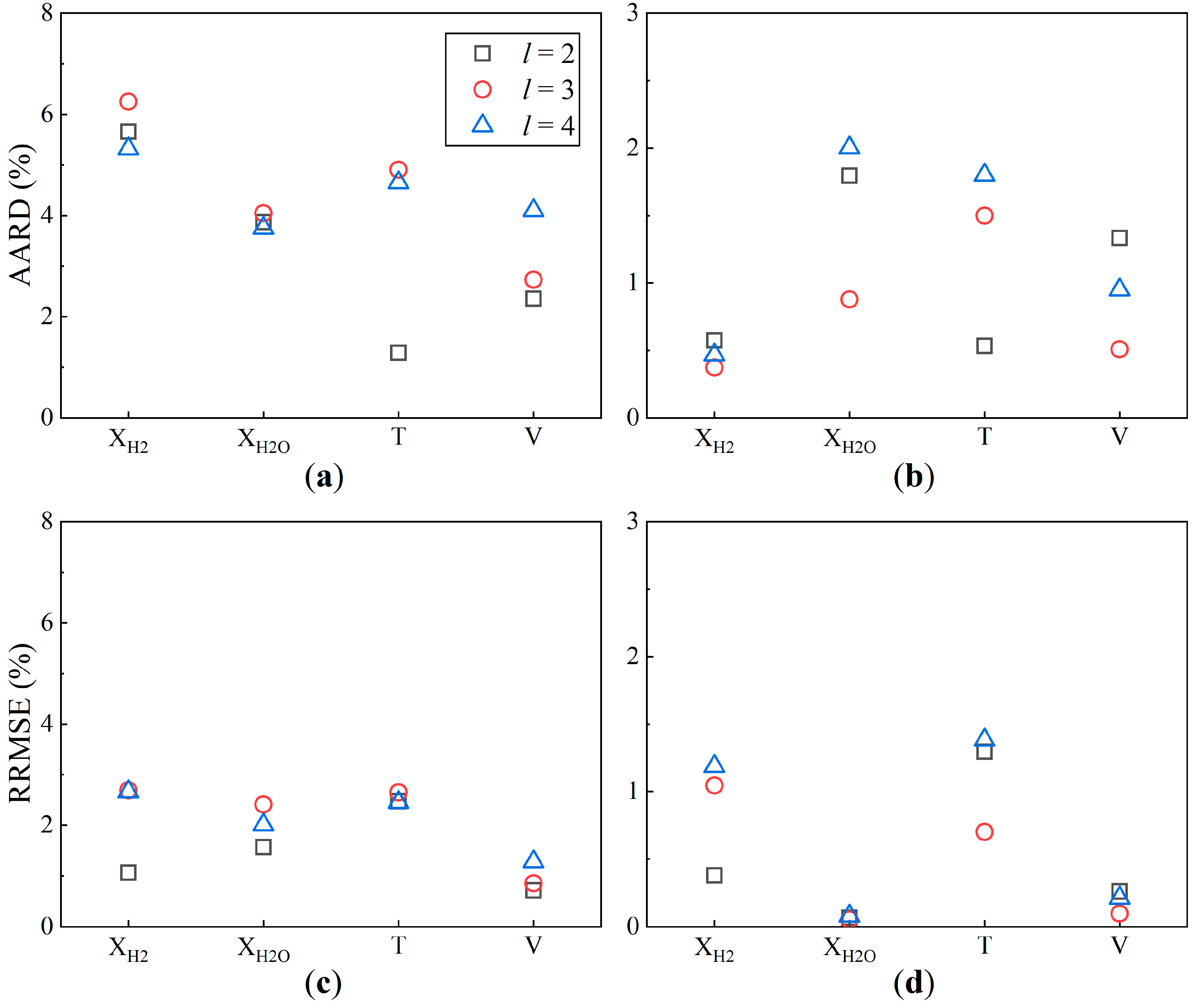
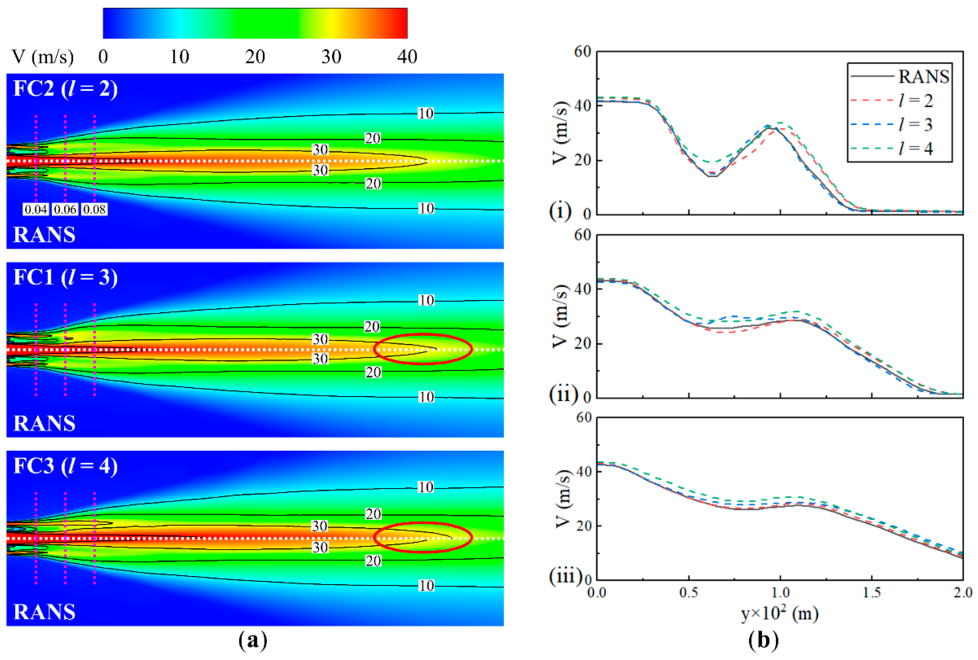
  • For AE-based ROMs, deeper networks are essential for capturing features in strongly nonlinear flowfields, while fewer layers are more effective for weakly nonlinear flowfields to avoid overfitting, as indicated by the average reconstruction AARDs. Specifically, when predicting a temperature field with strong nonlinearity, the l = 2 CAE model exhibited an absolute RD consistently ranging from 15% to 30% in the flame anchoring region, which was considerably larger than that of the l = 3 and 4 models. In contrast, for weakly nonlinear X H 2 predictions, an l = 2 configuration was more suitable.
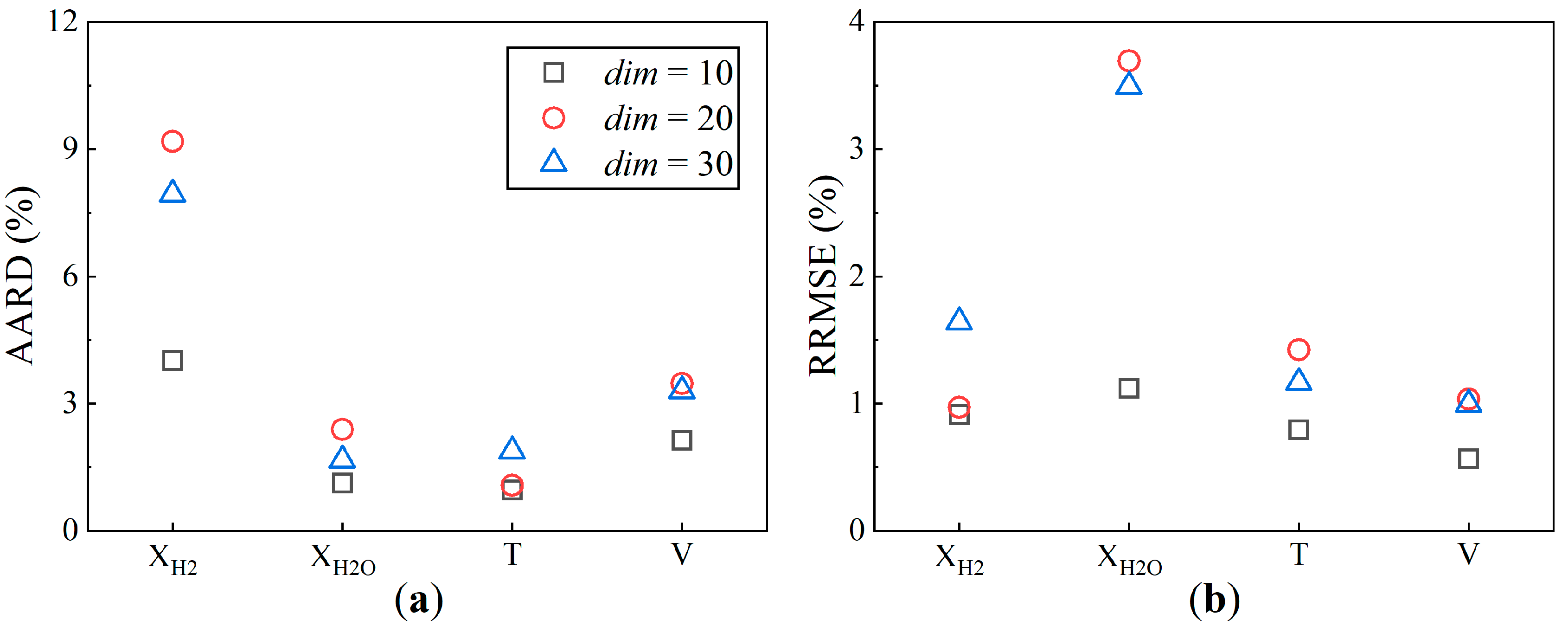
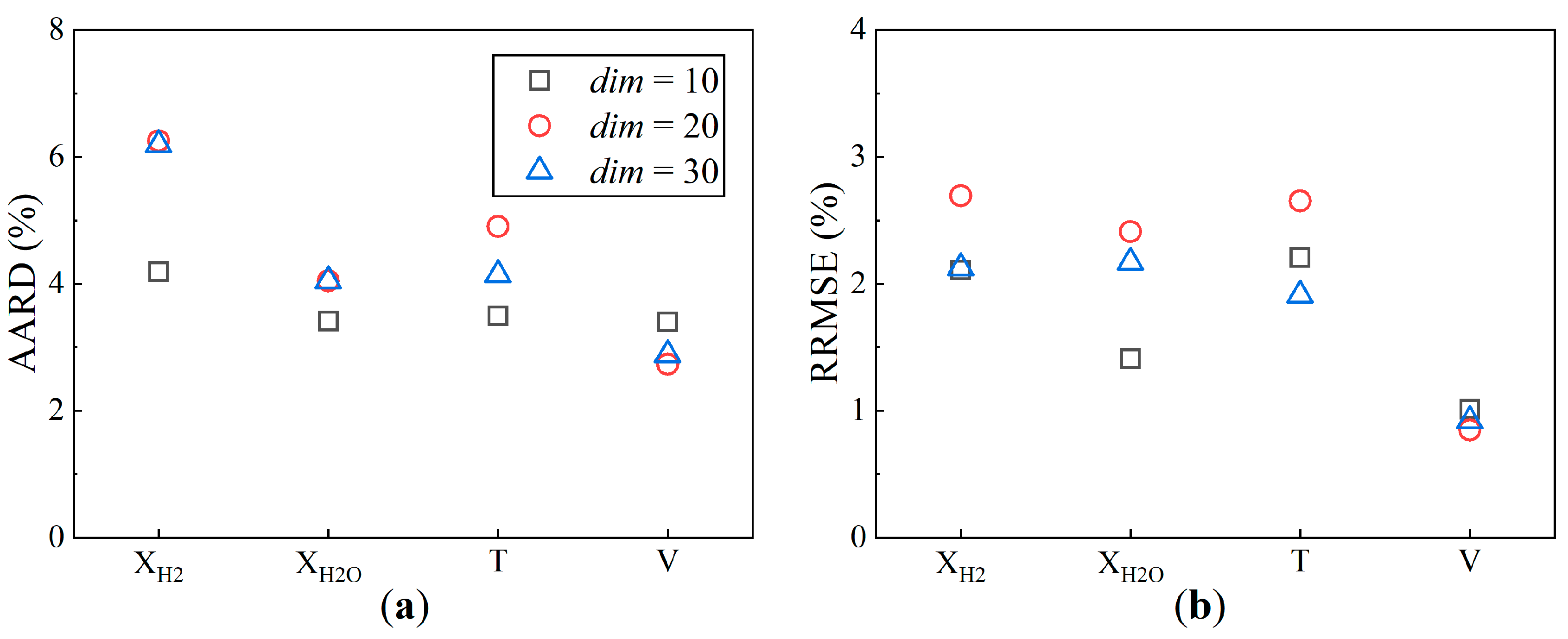
  • AE-based ROMs with fewer dimensions may yield better performance for flowfields where nonlinearity is less pronounced, while they may lead to an increased local error in certain cases because of excessive feature compression. The prediction for X H 2 demonstrated that the CAE model with a dim = 10 achieved a significantly lower AARD of 4.01%, representing about a 50% reduction compared to the dim = 20 and 30 models. However, when predicting regions with strong shear effects, the local errors of the dim = 10 and 20 CAE models were larger.
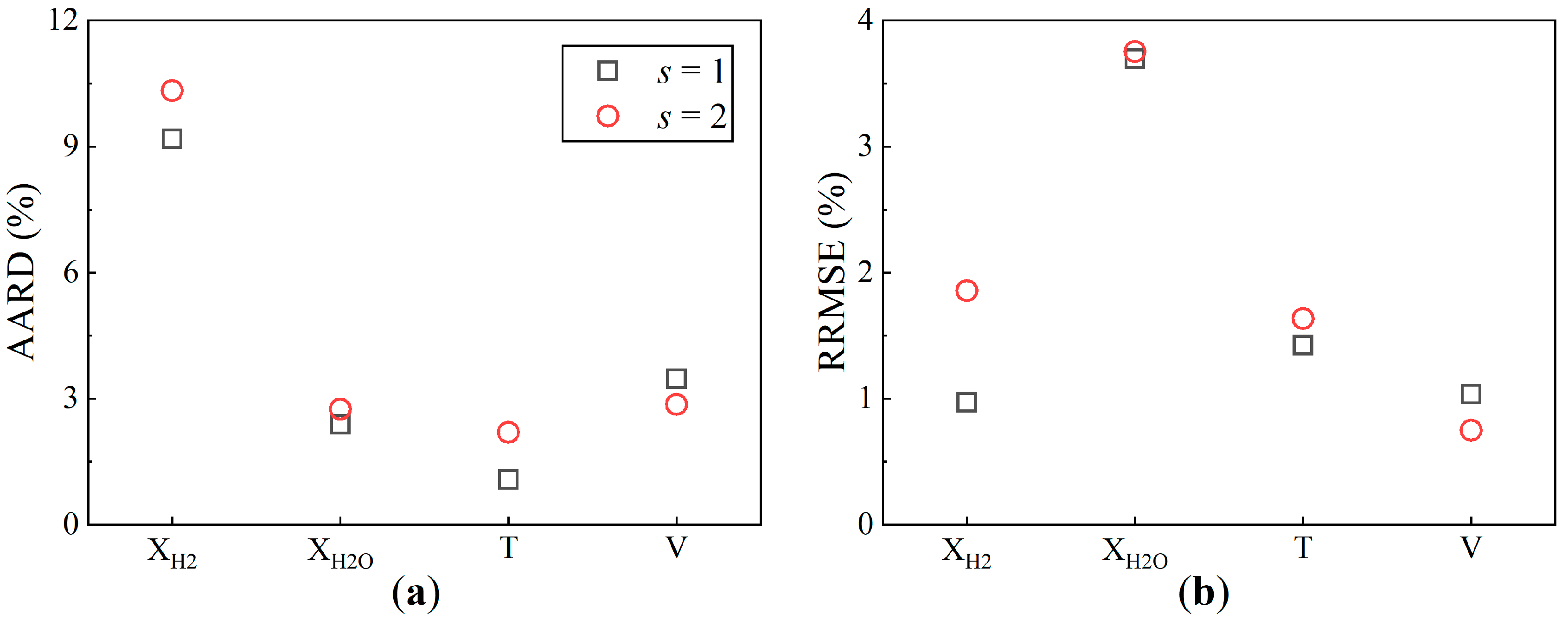
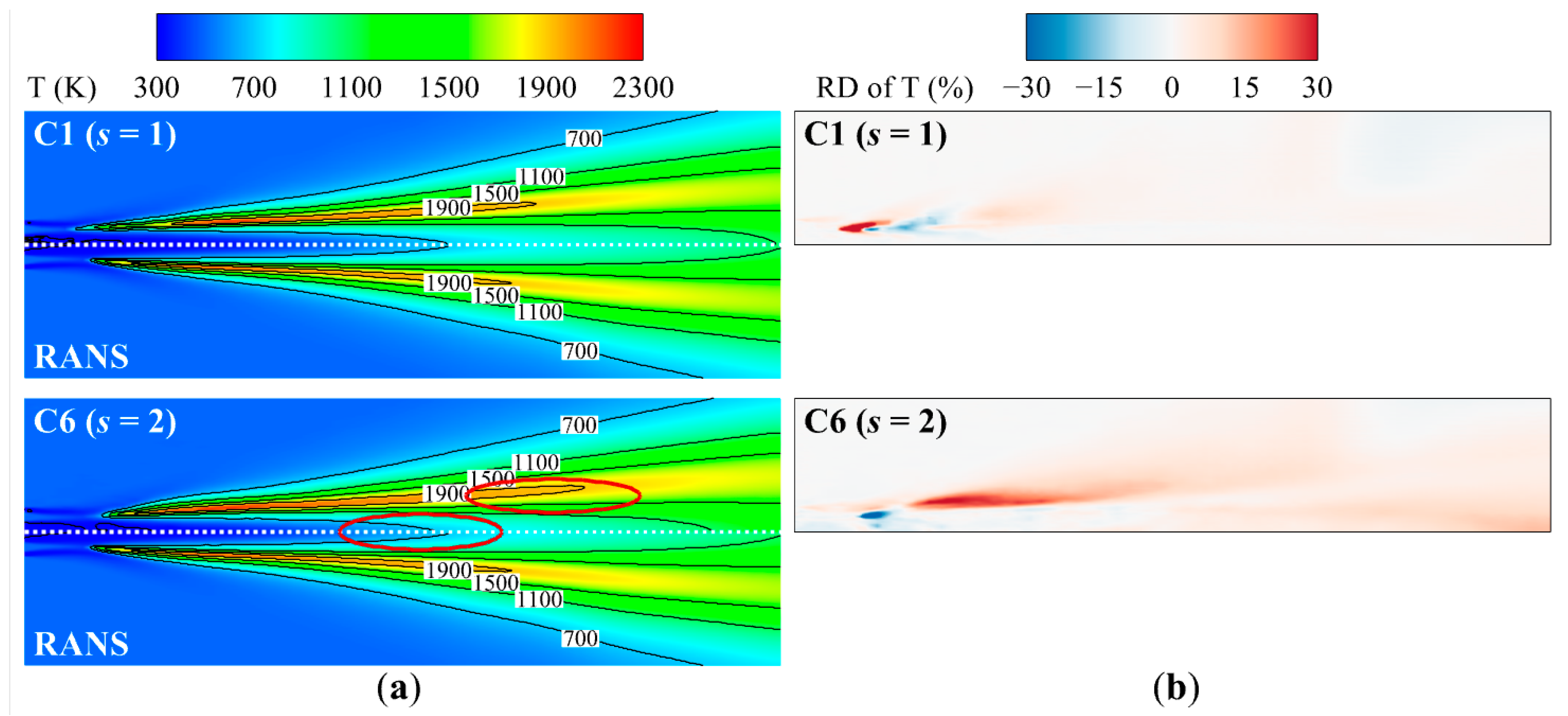
  • The CAE-based model indicated a preferable general simulation capability with a smaller convolutional stride, as the s = 1 model contained approximately 21 times more training parameters than the s = 2 model.
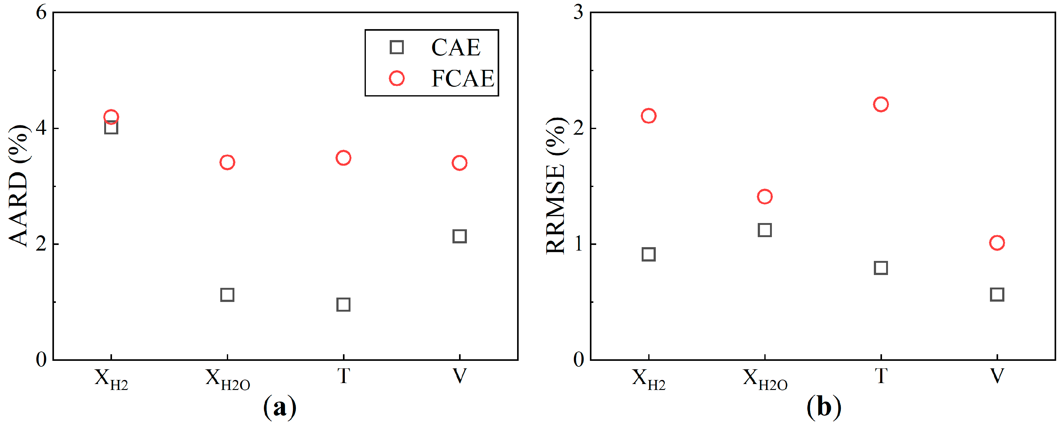
  • Comparing the CAE- and FCAE-based models under the same number of network layers and latent vector dimensionality, the CAE-based model exhibits superior predictive accuracy and a shorter training time.
This study offers valuable insights into hyperparameter settings for AE-based ROMs and clarifies the CAE model’s applicability for such a hydrogen-enriched combustion problem. The AE-based ROM developed in this study can be applied to datasets derived from other fuels or research domains, demonstrating its broad applicability. Future studies should further investigate the hyperparameter settings of AE-based ROMs for datasets from unstructured grids.

Author Contributions

Conceptualization, X.W.; methodology, X.C. and X.W.; software, L.Z. and X.C.; investigation, L.Z., X.C., S.D., M.Z. and C.N.; data curation, L.Z., X.C. and C.N.; writing—original draft preparation, L.Z. and X.C.; writing—review and editing, L.Z., X.C., S.D., M.Z. and X.W.; visualization, L.Z. and X.C.; supervision, X.W. and S.D.; project administration, X.W.; funding acquisition, X.W. All authors have read and agreed to the published version of the manuscript.

Funding

This research was partially supported by the Creative Seed Fund of the Shanxi Research Institute for Clean Energy, NO. 703 Research Institute of China State Shipbuilding Company, and the National Key Laboratory of Aerospace Liquid Propulsion.

Data Availability Statement

The original contributions presented in this study are included in the article. Further inquiries can be directed to the corresponding author.

Conflicts of Interest

The authors declare no conflicts of interest.

References

  1. Su-Ungkavatin, P.; Tiruta-Barna, L.; Hamelin, L. Biofuels, electrofuels, electric or hydrogen?: A review of current and emerging sustainable aviation systems. Prog. Energy Combust. Sci. 2023, 96, 101073. [Google Scholar]
  2. Jin, U.; Kim, K.T. Hybrid rich-and lean-premixed ammonia-hydrogen combustion for mitigation of NOx emissions and thermoacoustic instabilities. Combust. Flame 2024, 262, 113366. [Google Scholar] [CrossRef]
  3. Tanneberger, T.; Schimek, S.; Paschereit, C.O.; Stathopoulos, P. Combustion efficiency measurements and burner characterization in a hydrogen-oxyfuel combustor. Int. J. Hydrogen Energy 2019, 44, 29752–29764. [Google Scholar]
  4. Abbas, T.; Chen, S.; Zhang, X.; Wang, Z. Coordinated optimization of hydrogen-integrated energy hubs with demand response-enabled energy sharing. Processes 2024, 12, 1338. [Google Scholar] [CrossRef]
  5. Hydrogen Gas Turbines. Available online: https://etn.global/wp-content/uploads/2020/01/ETN-Hydrogen-Gas-Turbines-report.pdf (accessed on 18 February 2025).
  6. Lieuwen, T.; McDonell, V.; Petersen, E.; Santavicca, D. Fuel flexibility influences on premixed combustor blowout, flashback, autoignition and instability. Turbo Expo Power Land Sea Air 2006, 42363, 601–615. [Google Scholar]
  7. Noble, D.; Wu, D.; Emerson, B.; Sheppard, S.; Lieuwen, T.; Angello, L. Assessment of current capabilities and near-term availability of hydrogen-fired gas turbines considering a low-carbon future. J. Eng. Gas Turbines Power 2021, 143, 041002. [Google Scholar] [CrossRef]
  8. Noble, D.R.; Zhang, Q.; Shareef, A.; Tootle, J.; Meyers, A.; Lieuwen, T. Syngas mixture composition effects upon flashback and blowout. Turbo Expo Power Land Sea Air 2006, 42363, 357–368. [Google Scholar]
  9. Ni, C.; Ding, S.; Li, J.; Chu, X.; Ren, Z.; Wang, X. Projection-based reduced order modeling of multi-species mixing and combustion. Phys. Fluids 2024, 36, 077168. [Google Scholar]
  10. Ding, S.; Ni, C.; Chu, X.; Lu, Q.; Wang, X. Reduced-order modeling via convolutional autoencoder for emulating combustion of hydrogen/methane fuel blends. Combust. Flame 2025, 274, 113981. [Google Scholar]
  11. Li, J.; Zhang, R.; Wang, H.; Xu, Z. Inverse problem of permeability field under multi-well conditions using TgCNN-based surrogate model. Processes 2024, 12, 1934. [Google Scholar] [CrossRef]
  12. Forrester, A.I.; Keane, A.J. Recent advances in surrogate-based optimization. Prog. Aerosp. Sci. 2009, 45, 50–79. [Google Scholar]
  13. Eldred, M.; Dunlavy, D. Formulations for surrogate-based optimization with data fit, multifidelity, and reduced-order models. In Proceedings of the 11th AIAA/ISSMO Multidisciplinary Analysis and Optimization Conference, Portsmouth, VA, USA, 6–8 September 2006; p. 7117. [Google Scholar]
  14. Sun, L.; Gao, H.; Pan, S.; Wang, J.-X. Surrogate modeling for fluid flows based on physics-constrained deep learning without simulation data. Comput. Methods Appl. Mech. Eng. 2020, 361, 112732. [Google Scholar]
  15. Ma, T.; Lu, H.; Li, Q. Optimization design method based on parameter reduction and active subspaces: Redistribution of chordwise loading at blade tips in a transonic axial-flow fan. Phys. Fluids 2024, 36, 095103. [Google Scholar]
  16. Hou, C.K.J.; Behdinan, K. Dimensionality reduction in surrogate modeling: A review of combined methods. Data Sci. Eng. 2022, 7, 402–427. [Google Scholar]
  17. Berkooz, G.; Holmes, P.; Lumley, J.L. The proper orthogonal decomposition in the analysis of turbulent flows. Annu. Rev. Fluid Mech. 1993, 25, 539–575. [Google Scholar]
  18. Benner, P.; Gugercin, S.; Willcox, K. A survey of projection-based model reduction methods for parametric dynamical systems. SIAM Rev. 2015, 57, 483–531. [Google Scholar]
  19. Wang, X.; Chang, Y.-H.; Li, Y.; Yang, V.; Su, Y.-H. Surrogate-based modeling for emulation of supercritical injector flow and combustion. Proc. Combust. Inst. 2021, 38, 6393–6401. [Google Scholar]
  20. Hinton, G.E.; Salakhutdinov, R.R. Reducing the dimensionality of data with neural networks. Science 2006, 313, 504–507. [Google Scholar]
  21. Milan, P.J.; Torelli, R.; Lusch, B.; Magnotti, G. Data-driven model reduction of multiphase flow in a single-hole automotive injector. At. Sprays 2020, 30, 401–429. [Google Scholar]
  22. Brunton, S.L.; Noack, B.R.; Koumoutsakos, P. Machine learning for fluid mechanics. Annu. Rev. Fluid Mech. 2020, 52, 477–508. [Google Scholar]
  23. Xu, J.; Duraisamy, K. Multi-level convolutional autoencoder networks for parametric prediction of spatio-temporal dynamics. Comput. Methods Appl. Mech. Eng. 2020, 372, 113379. [Google Scholar]
  24. Hartman, D.; Mestha, L.K. A deep learning framework for model reduction of dynamical systems. In Proceedings of the 2017 IEEE Conference on Control Technology and Applications (CCTA), Hawaii, HI, USA, 27–30 August 2017; IEEE: Piscataway, NJ, USA, 2017; pp. 1917–1922. [Google Scholar]
  25. Agostini, L. Exploration and prediction of fluid dynamical systems using auto-encoder technology. Phys. Fluids 2020, 32, 067103. [Google Scholar]
  26. Zhang, Y.; Chen, Y.; Wang, J.; Pan, Z. Unsupervised deep anomaly detection for multi-sensor time-series signals. IEEE Trans. Knowl. Data Eng. 2021, 35, 2118–2132. [Google Scholar]
  27. Nakamura, T.; Fukami, K.; Hasegawa, K.; Nabae, Y.; Fukagata, K. Convolutional neural network and long short-term memory based reduced order surrogate for minimal turbulent channel flow. Phys. Fluids 2021, 33, 025116. [Google Scholar]
  28. Milano, M.; Koumoutsakos, P. Neural network modeling for near wall turbulent flow. J. Comput. Phys. 2002, 182, 1–26. [Google Scholar]
  29. Lee, K.; Carlberg, K.T. Model reduction of dynamical systems on nonlinear manifolds using deep convolutional autoencoders. J. Comput. Phys. 2020, 404, 108973. [Google Scholar]
  30. Gruber, A.; Gunzburger, M.; Ju, L.; Wang, Z. A comparison of neural network architectures for data-driven reduced-order modeling. Comput. Methods Appl. Mech. Eng. 2022, 393, 114764. [Google Scholar]
  31. Ding, S.; Wang, L.; Lu, Q.; Wang, X. Data-driven surrogate modeling and optimization of supercritical jet into supersonic crossflow. Chin. J. Aeronaut. 2024, 37, 139–155. [Google Scholar]
  32. Wu, X.; Wu, S.; Tian, X.; Guo, X.; Luo, X. Effects of hyperparameters on flow field reconstruction around a foil by convolutional neural networks. Ocean Eng. 2022, 247, 110650. [Google Scholar]
  33. Fukami, K.; Hasegawa, K.; Nakamura, T.; Morimoto, M.; Fukagata, K. Model order reduction with neural networks: Application to laminar and turbulent flows. SN Comput. Sci. 2021, 2, 467. [Google Scholar]
  34. Lui, H.; Wolf, W. Convolutional neural networks for the construction of surrogate models of fluid flows. In Proceedings of the AIAA Scitech 2021 Forum, Virtual, 11–21 January 2021; p. 1675. [Google Scholar]
  35. Peng, J.-Z.; Chen, S.; Aubry, N.; Chen, Z.; Wu, W.-T. Unsteady reduced-order model of flow over cylinders based on convolutional and deconvolutional neural network structure. Phys. Fluids 2020, 32, 123609. [Google Scholar]
  36. Wang, L.; Xiao, H.; Yang, B.; Wang, X.-E. Steam dilution effect on laminar flame characteristics of hydrogen-enriched oxy-combustion. Int. J. Hydrogen Energy 2024, 71, 375–386. [Google Scholar]
  37. McGuinness, R.M.; Kleinberg, W.T. Oxygen Production. In Oxygen-Enhanced Combustion, 2nd ed.; CRC Press: Boca Raton, FL, USA, 2013; pp. 92–125. [Google Scholar]
  38. Gregory, P.; Smith, D.M.G.; Frenklach, M.; Moriarty, N.W.; Eiteneer, B.; Goldenberg, M.; Bowman, C.T.; Hanson, R.K.; Song, S.; Gardiner, W.C.; et al. Available online: http://www.me.berkeley.edu/gri_mech/ (accessed on 18 February 2025).
  39. Undapalli, S.; Srinivasan, S.; Menon, S.-I. LES of premixed and non-premixed combustion in a stagnation point reverse flow combustor. Proc. Combust. Inst. 2009, 32, 1537–1544. [Google Scholar]
  40. Gopalakrishnan, P.; Bobba, M.; Seitzman, J.-I. Controlling mechanisms for low NOx emissions in a non-premixed stagnation point reverse flow combustor. Proc. Combust. Inst. 2007, 31, 3401–3408. [Google Scholar]
  41. Glorot, X.; Bordes, A.; Bengio, Y. Deep sparse rectifier neural networks. In Proceedings of the Fourteenth International Conference on Artificial Intelligence and Statistic, Fort Lauderdale, FL, USA, 11–13 April 2011; pp. 315–323. [Google Scholar]
  42. Mak, S.; Sung, C.-L.; Wang, X.; Yeh, S.-T.; Chang, Y.-H.; Joseph, V.R.; Yang, V.; Wu, C.J. An efficient surrogate model for emulation and physics extraction of large eddy simulations. J. Am. Stat. Assoc. 2018, 113, 1443–1456. [Google Scholar]
  43. Zhou, M.; Ni, C.; Sung, C.-L.; Ding, S.; Wang, X. Modeling of thermophysical properties and vapor-liquid equilibrium using Gaussian process regression. Int. J. Heat Mass Transf. 2024, 219, 124888. [Google Scholar]
  44. Cheng, J.C.; Wang, M. Automated detection of sewer pipe defects in closed-circuit television images using deep learning techniques. Autom. Constr. 2018, 95, 155–171. [Google Scholar]
Figure 1. Triple-coaxial injection nozzle configuration.
Processes 13 01093 g001
Figure 2. Comparison of axial velocity profiles between experiment and numerical simulations at x = 113 mm.
Processes 13 01093 g002
Figure 3. Centerline variations in temperature for different mesh sizes.
Processes 13 01093 g003
Figure 4. Design points (training cases) and test cases in the design space.
Processes 13 01093 g004
Figure 5. Structures of (a) CAE-based ROM and (b) FCAE-based ROM.
Processes 13 01093 g005
Figure 6. Average (a) prediction AARDs, (b) reconstruction AARDs, (c) prediction RRMSEs, and (d) reconstruction RRMSEs of physical fields achieved by CAE-based ROMs C1 (l = 3), C2 (l = 2), and C3 (l = 4).
Processes 13 01093 g006
Figure 7. (a) Spatial distributions of temperature predicted by CAEs (upper) and obtained from numerical simulation (lower); (b) spatial distributions of temperature RD predicted by CAE models; (c) spatial distributions of x-direction velocity gradient with respect to x-direction from RANS simulation for test case 2 ( X C H 4 = 0.5 ,   H 2 O = 0.15 ).
Processes 13 01093 g007
Figure 8. Average (a) prediction AARDs and (b) prediction RRMSEs of physical fields achieved by CAE-based ROMs C1 (dim = 20), C4 (dim = 10), and C5 (dim = 30).
Processes 13 01093 g008
Figure 9. Spatial distributions of X H 2 (a) predicted by CAEs (upper) and obtained from numerical simulation (lower); (b) RD predicted by CAE models for test case 1 ( X C H 4 = 0.3 ,   H 2 O = 0.15 ).
Processes 13 01093 g009
Figure 10. Average (a) prediction AARDs and (b) prediction RRMSEs of physical fields achieved by CAE-based ROMs C1 (s = 1) and C6 (s = 2).
Processes 13 01093 g010
Figure 11. Spatial distributions of temperature (a) predicted by CAEs (upper) and obtained from numerical simulation (lower); (b) RD predicted by CAE models for test case 3 ( X C H 4 = 0.5 ,   H 2 O = 0.25 ).
Processes 13 01093 g011
Figure 12. Average (a) prediction AARDs, (b) reconstruction AARDs, (c) prediction RRMSEs, and (d) reconstruction RRMSEs of physical fields achieved by FCAE-based ROMs FC1 (l = 3), FC2 (l = 2), and FC3 (l = 4).
Processes 13 01093 g012
Figure 13. Spatial distributions of velocity magnitude (a) predicted by FCAEs (upper) and obtained from numerical simulation (lower) and (b) predicted by models and obtained from numerical simulation at axial positions of (i) x = 0.04 m, (ii) x = 0.06 m, and (iii) x = 0.08 m for test case 4 ( X C H 4 = 0.7 ,   H 2 O = 0.25 ).
Processes 13 01093 g013
Figure 14. Average (a) prediction AARDs and (b) prediction RRMSEs of physical fields achieved by FCAE-based ROMs FC1 (dim = 20), FC4 (dim = 10), and FC5 (dim = 30).
Processes 13 01093 g014
Figure 15. Spatial distributions of X H 2 (a) predicted by FCAEs (upper) and obtained from numerical simulation (lower); (b) RD predicted by FCAE models for test case 4 ( X C H 4 = 0.7 ,   H 2 O = 0.25 ).
Processes 13 01093 g015
Figure 16. Average (a) prediction AARDs and (b) prediction RRMSEs of physical fields achieved by CAE- and FCAE-based ROMs C4 and FC4.
Processes 13 01093 g016
Figure 17. Spatial distributions of (a) temperature and (b) X H 2 O predicted by CAE and FCAE (upper) and obtained from numerical simulation (lower) for test case 2 ( X C H 4 = 0.5 ,   H 2 O = 0.15 ).
Processes 13 01093 g017
Table 1. Geometric settings.
StructuresSize (mm)
Outer Diameter of Fuel Nozzle, D 1 9
Outer Diameter of Steam Nozzle, D 2 16
Outer Diameter of Oxygen Nozzle, D 3 22
Thickness of Nozzle Wall, d 1
Axial Span of Computational Domain, L x 360
Radial Span of Computational Domain, L y 160
Table 2. Hyperparameter settings for CAE and FCAE models.
Model NumberLDimS
CAEC13201
C22201
C34201
C43101
C53301
C63202
FCAEFC1320/
FC2220/
FC3420/
FC4310/
FC5330/
Table 3. Total number of parameters and training time of all CAE-based ROMs.
CAE-Based ROMsTotal Training ParametersTraining Time (s)
C11,476,22959,671
C25,772,837143,168
C3433,38147,530
C4779,89954,783
C52,172,55966,424
C669,8938751
Table 4. Number of training parameters, training time, and prediction time of C4 and FC4, along with simulation time.
AETotal Training ParametersTraining Time (s)Prediction Time (ms)Simulation Time (CPUh)
C4779,89954,7833.916288–576
FC4293,473,0461,892,76711.860
Disclaimer/Publisher’s Note: The statements, opinions and data contained in all publications are solely those of the individual author(s) and contributor(s) and not of MDPI and/or the editor(s). MDPI and/or the editor(s) disclaim responsibility for any injury to people or property resulting from any ideas, methods, instructions or products referred to in the content.

