A Mobile Energy Storage Configuration Method for Power Grids Considering Power Losses and Voltage Stability

Abstract

The generation output of distributed power sources and the load possess periodic changes, which cause stability problems in the operation of the power grid. To ensure stability, energy storage devices are generally installed in the power grid, but their effectiveness is also limited by their fixed installation location and capacity. In this paper, to overcome the drawback of stationary energy storage devices, mobile energy storage devices are introduced to reduce power losses and enhance voltage stability. The installation location and capacity of these mobile energy storage devices can be changed with the generation output and load demands. Firstly, the influence of the mobile energy storage devices on power losses and voltage stability is analyzed. Next, a multi-objective optimization model is established to select the optimal installation location and the ideal capacity, which has optimization objectives including the improvement of voltage stability, the minimization of power losses, and the enhancement of utilization of energy storage devices. Finally, the particle swarm optimization algorithm is applied to solve the multi-objective optimization problem. The simulation results prove that the novel method of this paper enhances the dynamics of the power grid, i.e., the voltage vulnerability and power losses are reduced by 29% and 36%, respectively. In addition, it also increases the utilization rate of energy storage devices by 33.5% in different operating scenarios.

1. Introduction

Because of the rapid development of renewable energy, a larger number of distributed power sources are being integrated into the power grid. However, these renewable energy sources are characterized by fluctuations. For instance, wind power generation relies on wind resources, and the instability of wind power generation results in fluctuations in power output. Similarly, photovoltaic power generation relies on the intensity and duration of sunlight, and its capacity for generating electricity decreases significantly on cloudy days or during nighttime. For example, the “Zhangbei Renewable Energy Base” is one of the largest renewable energy demonstration bases in China, which includes wind and photovoltaic power generation and achieves a high percentage of renewable energy by connecting to the grid utilizing smart grid technology [1]. Due to the randomness of distributed generation, its large-scale integration poses challenges to the stability of the power grid [2,3,4,5]. This randomness often leads to some technical problems in the distribution network, including voltage imbalance, power loss, and reversed power flow. When the demand for electricity is low, the new energy generation system continuously supplies power to the grid, which increases the system voltage. This leads to shortened equipment lifetimes, tripping, or equipment damage. In terms of load demands, there are variations in electricity consumption at different times, characterized by peaks and troughs. The rapid growth of emerging loads, such as the electric vehicle charging stations, further exacerbates the uncertainty of load demands [6,7,8,9]. The fluctuations of the distributed generation output and the load demands show the characteristic of periodic changes and bring about stability problems in the power grid [10]. To balance supply and demand in real time and reduce fluctuations, one of the most effective solutions to the stability problem is the installation of energy storage devices [5,11]. As flexible power regulation equipment, energy storage devices store excess energy when load demands are low and release it when demands are high. Therefore, the introduction of energy storage devices can balance the load demand and generation output and can maintain the voltage stability of the power grid. Therefore, the study of the application of energy storage devices to the power system is essential for the operation of power grids.

1.1. Literature Review

The suitable installation location and the allowable minimum capacity of energy storage devices in the power grid are the main concerns for the configuration, which has been researched in the past few decades with numerous studies proposed. Sanjay et al. used the hybrid gray wolf optimization algorithm to determine the optimal configuration of distributed generator sets [12]. Khan et al. used an improved grey wolf optimizer to determine the optimal distributed generation (DG) allocation in order to reduce the power losses of the power grid [13]. Onlam et al. employed an adaptive optimization algorithm to address the DG configuration problem, aiming to reduce power losses and enhance voltage stability [14]. Sangeeta et al. proposed a sensitivity analysis method for voltage stability to determine the optimal location for DG [15]. Carpinelli et al. analyzed the benefits of integrating energy storage devices into the grid but did not consider the impact of energy storage devices on the power grid [16]. Ghofrani et al. studied the economic effects of energy storage devices on the grid, but they did not consider its impact on voltage stability [17]. Ahmed et al. determined the optimal size and location of DG and PV with the goal of minimizing costs without considering the stability of the grid [18]. In order to restrain the fluctuation of wind power and reduce the economic cost of the energy storage system, Yuming et al. proposed an optimization method to choose the optimal capacity, which also did not take into account the stability of the power grid [19]. Zhang et al. used the adaptive grey wolf optimization algorithm to determine the location and capacity of energy storage devices for the purpose of improving system reliability and voltage frequency stability, but this paper did not consider economic factors [20].

Most research focuses on stationary energy storage devices whose installation location and capacity cannot be changed with varying load demands; therefore, the effectiveness of stationary energy storage devices is limited if the operating scenario changes. Fortunately, mobile energy storage technology provides a way to overcome the drawbacks of stationary energy storage devices; however, little attention has been paid to this. As stated in [21], electric vehicles are typical mobile energy storage devices that can be used to improve the stability of power grids through vehicle-to-grid (V2G) technology. Therefore, electric vehicles can be considered a practical application of mobile energy storage devices. For example, in [22,23], the optimal capacity of the mobile energy storage devices of electric vehicles and the plan of charge or discharge were investigated for the stability problem of the power grid. In [24], the connection of electric vehicles with the power grid through V2G technology was studied, showing a positive influence on the integration of photovoltaic power generation. Meanwhile, by considering the mobile energy storage devices in the power grid, the configuration problem was investigated with regard to economic benefits [25]. By considering the lowest fluctuation of power as the optimization objective, the optimal capacity of energy storage devices was investigated [26]. By taking the largest economic benefits as the objective, the optimal location and capacity were determined using mixed-integer second-order cone programming [27].

Based on the analysis of the above, it is found that most previous research has been on stationary energy storage devices. Secondly, research on the configuration of mobile energy storage devices in the power grid does not attract enough attention and there is still room for further study. As for the configuration of mobile energy storage devices, the main focus is on the economic aspects of power grid operation, but few studies address the effect of mobile energy storage devices on the voltage stability and power losses of power grid operation in depth. Therefore, this paper aims to further explore how to determine the optimal configuration of mobile energy storage devices to enhance the voltage stability of power grids and reduce power losses, which are essential for the stable operation of power grids.

1.2. Contributions

As for the fluctuations of load demands and the distributed generation output, mobile energy storage technology provides an effective way of improving the stability of the power grid by adjusting the installation location and capacity according to the operation. In this paper, a mobile energy storage configuration method is proposed to enhance the utilization rate of the mobile energy storage devices and grid stability.

The major contributions of this paper are as follows:

(1)

Firstly, this study investigates the impact of energy storage devices on voltage stability and power losses with changes in the installation location and the capacity, which has not been studied in previous research;

(2)

Secondly, by fully considering the properties of the load demand of the power grid within a day, the load period is divided into three load scenarios, i.e., low, flat, and peak, and then a multi-objective optimization model is established to determine the optimal position and ideal capacity of energy storage devices for three different scenarios. The optimization objectives include the minimization of power loss, the improvement of voltage stability, and the improvement of the utilization of energy storage devices;

(3)

Finally, the IEEE 33-node system is used for the simulation in MATLAB R2023a. By comparing the simulation results of the stationary energy storage and the mobile energy storage, it is verified that the proposed method effectively improves the voltage stability and utilization rate of energy storage devices and reduces power losses.

1.3. Research Methodology

To make this paper readable,

Table 1. Conceptual framework of this study.

1. Research problem	The stability problem of the power grid caused by the fluctuation of new energy generation and load.
2. Research objectives	Main objectives: To determine the optimal configuration of mobile energy storage devices to enhance power grid stability.
	Specific objectives: To improve the voltage stability and utilization rate of energy storage devices and reduce power losses.
3. Research method	A mobile energy storage method by optimizing the optimal location and capacity of energy storage.
4. Techniques and tools	Multi-objective particle swarm optimization: Solving multi-objective optimization problems. Matlab R2023a: For simulation and example analysis.
5. Simulation	Simulation objects: Take the IEEE 33-node system (including wind turbines, photovoltaic generators, and energy storage devices) as an example. The stationary energy storage device and the mobile energy storage device are used as simulation objects. Simulation results: The voltage vulnerability and power losses are reduced by 29% and 36%, respectively. The utilization rate of energy storage devices increases by 33.5%.

shows the research problem, research objectives, research method, techniques, tools, and simulation.

1.4. Organization

The rest of this paper is organized as follows. In Section 2, the influence of mobile energy storage devices on the power grid and the characteristics of mobile energy storage devices are analyzed. In Section 3, a multi-objective optimization model is proposed to determine the optimal location and capacity of the energy storage device. In Section 4, particle swarm optimization (PSO) is introduced for solving multi-objective optimization problems. In Section 5, the validity of the proposed method is verified by simulation analysis. Finally, the conclusions are presented in Section 6.

2. The Influence of Mobile Energy Storage Devices on the Power Grid and the Characteristics of Mobile Energy Storage Devices

To prove the usefulness of mobile energy storage devices, the influence of introducing mobile energy storage devices on voltage stability and power losses is studied, and their characteristics are also introduced.

2.1. The Influence of Mobile Energy Storage Devices on the Power Grid

Integrating energy storage devices into the power grid enhances both its safety and economy. These devices charge or discharge according to load demands to improve voltage stability [28]. Additionally, power losses are related to the grid voltage. These losses increase or decrease in accordance with fluctuations in voltage levels [29,30]. Utilizing mobile energy storage devices to deal with fluctuations in distributed power sources and loads greatly reduces power losses and enhances voltage stability. Therefore, the impact of mobile energy storage devices on power losses and voltage stability is discussed in this section, which provides insights for the following research.

In the following example, the IEEE 33-node system is used in a simulation to study the influence of energy storage devices on voltage and power losses during the discharge state. The influence of energy storage devices on voltage and power losses at various locations and capacities is shown in Figure 1. The nodes in various colors represent the different positions of the energy storage device. According to part (a) of Figure 1, for all nodes, the voltage increases as the capacity increases, but the location changes lead to complicated influences on the voltage. For example, when the capacity is 1000 kWh, the voltage of node 13 is significantly higher than the other nodes, but when the capacity is 3000 kWh, the voltage of node 6 becomes the highest. Part (b) of Figure 1 indicates that energy storage devices with an appropriate capacity can effectively reduce power losses. However, as the capacity continues to increase, power losses also rise. For instance, when the capacity is less than 100 kWh, the location has little influence on power losses; however, when the capacity exceeds 1000 kWh, the influence on power loss becomes more pronounced at nodes 13 and 18.

Although large-capacity energy storage devices are effective in improving voltage stability, excessive capacity leads to an increase in power losses and higher investment costs, as well as the movement of devices. The capacity should be reduced as little as possible while ensuring the improvement of voltage stability. Therefore, when determining the location and capacity of energy storage devices, voltage stability and power losses cannot be ignored.

2.2. Analysis of the Characteristics of Mobile Energy Storage Devices

Previous research has mainly focused on stationary energy storage devices. These devices have some limitations when installed in fixed locations, which limits their applications in power systems. The construction of stationary energy storage devices also requires careful consideration of factors such as location, land availability, and infrastructure. If there are discrepancies between the predicted demands and the actual demands, the cost of subsequent adjustments is high.

With the development of high-energy batteries and intelligent energy management systems, the installation location and the capacity of energy storage devices can be changed [22]. When mobile energy storage devices are deployed, their capacity, power, and location can be adjusted to meet the specific demands of different situations, which significantly improves the utilization rate of these devices [31].

To accurately reflect the utilization rate of energy storage devices, Formula (1) is employed to quantify this rate. A higher utilization rate indicates a longer operational time. The utilization rate is calculated as follows:

$$\beta ={\displaystyle \frac{T_{use}}{T_{all}}}$$

(1)

where $T_{use}$ is the operating time of energy storage devices within a research cycle, and $T_{all}$ is the duration of one research cycle.

The mobile energy storage devices utilized in this paper consist of a number of energy storage battery units. Its design is convenient for disassembly and installation, and the number of devices can be increased according to the total capacity required to avoid the energy waste caused by the excessive distributed generation output. Because of their high energy density, these energy storage devices have a variety of advantages in volume and can be flexibly arranged in different locations according to the needs of various scenarios.

According to the characteristics of mobile energy storage devices, a management center is established within the power grid. When the location and capacity of energy storage need to be changed to meet different demands, this center serves as a platform for the coordination and maintenance of energy storage devices. Initially, devices will be adjusted between nodes within the network. Subsequently, new devices will be dispatched from the management center, or unused devices will be returned to the management center based on load demands. The overall configuration method is illustrated in Figure 2.

3. Multi-Objective Optimization Model for the Determination of the Optimal Location and Capacity of the Energy Storage Devices

The determination of the optimal location and capacity is a multi-objective optimization problem. In Section 2, the location and capacity changes of energy storage devices have been proven to have an obvious influence on the voltage stability and values of power losses. On this basis, it is important to ensure the proper configuration of mobile energy storage devices to realize voltage stability, a reduction in power losses, and an increase in the utilization rate. In this paper, voltage vulnerability is introduced to quantify the voltage stability. The smaller the voltage vulnerability, the more stable the system. The smaller the power loss and the capacity of energy storage devices, the lower the investment cost. The multi-objective optimization model for the determination of the optimal location and capacity of the energy storage devices is established in this paper and its objective function and constraints are shown below.

3.1. Objective Functions

(1)

Voltage stability

During the operation of the power grid, disturbances lead to voltage instability, causing the voltage of each node to deviate from the normal range. Therefore, in order to minimize these impacts, voltage vulnerability is introduced to measure voltage stability as an objective function. Voltage vulnerability is derived from the standard voltage deviation at each node within the power grid and serves as a measure of voltage stability. A higher voltage vulnerability indicates poorer voltage quality at the node [29,32,33]. The process for constructing the voltage vulnerability is as follows:

$$\left\{\begin{array}{c}v\left(t,j\right)={\displaystyle \frac{{|U}_{t,j}-U_{e,j}|}{∆U_{max}}}\\ V_{\left(t,j\right)}={\displaystyle \frac{v\left(t,j\right)-v\left(t,j_{min}\right)}{v\left(t,j_{max}\right)-v\left(t,j_{min}\right)}}\end{array}\right.$$

(2)

$$B\left(t\right)={\displaystyle \frac{1}{N}}\sum _{j=1}^{N}V\left(t,j\right)$$

(3)

$$f_1={\displaystyle \frac{1}{T}}\sum _{t=1}^{T}B\left(t\right)$$

(4)

where $U_{e,j}$ is the rated voltage of node $j$, $v(t,j)$ and $U_{t,j}$ are the voltage vulnerability and rated voltage of node $j$ at time $t$, respectively, $∆U_{max}$ is the maximum allowable voltage deviation, $V(t,j)$ is the voltage vulnerability of node $j$ after standardization at time $t$, $v(t,j_{max})$ and $v(t,j_{min})$ represent the maximum and minimum voltage vulnerability values of all nodes at time $t$ before standardization, respectively, $B\left(t\right)$ is the integrated voltage vulnerability at time $t$, $T$ is the unit cycle of the system operation with $T=24$, and $N$ is the number of nodes of the system.

The average voltage vulnerability $f_1$ ranges from 0 to 1. A higher value indicates greater vulnerability, signifying the decreased security of the power grid. A value close to 0 reflects that the power grid’s operation is more stable and reliable.

(2)

Power loss

Power loss is an important research objective in power system research. The minimization of power loss is essential for improving system efficiency [32,34]. According to the load demands, energy storage devices either inject or absorb power at various nodes. This process redistributes power flow from overloaded lines to those with lighter loads, thereby reducing the current in the overloaded lines and minimizing power losses. The power loss is calculated as follows:

$$P_{loss}=\sum _{l=1}^L{k}_{t,l}\cdot r_l$$

(5)

$$f_2=\sum _{t=1}^T{P}_{loss}$$

(6)

where $P_{loss}$ represents power losses within one hour, $L$ represents the total count of lines within the power grid, $k_{t,l}$ is the square of the current in the line $l$ after the energy storage device is connected, and $r_l$ is the resistance of the line $l$.

(3)

Capacity of energy storage devices

The total capacity of energy storage devices must be carefully determined. If the capacity is too small, these devices will be unable to effectively enhance voltage stability, particularly during significant load changes. Conversely, if the capacity is too large, it will lead to an increase in investment costs. Therefore, the appropriate choice of capacity is crucial. The designated capacities of energy storage devices are defined by the maximum charge or discharge energy within the operational cycle. The capacity is determined by the following formula:

$$f_3=\sum _{m=1}^M\sum _{t=t_0}^{t_0+∆t}{P}_i\left(t\right)\cdot ∆t$$

(7)

where $t_0$ and $t_0+∆t$ are the start and end times of charging or discharging, respectively, $P_i\left(t\right)$ is the power of the storage device $i$ at time $t$, $∆t$ is the time interval between the start and end moments, and $M$ is the number of energy storage devices.

The multi-objective optimization functions, encompassing voltage stability, power losses, and the capacity of energy storage devices, are formulated as follows:

$$\mathit{min} f=\left[f_1,f_2,f_3\right]$$

(8)

3.2. Constraint Conditions

The constraints of the multi-objective optimization model are divided into two components: operation constraints of the power grid and the energy storage devices. The power grid operation constraints include both power flow balance constraints and power balance constraints. The energy storage devices’ operation constraints include both capacity and power constraints, as well as state of charge (SOC) constraints.

(1)

Power flow balance constraint

$$\left\{\begin{array}{c}{P}_i\left(t\right)=V_i\left(t\right){\displaystyle \sum _{j\in i}}{V}_i\left(t\right)\left(G_{i,j}{\mathit{cos}\theta }_{i,j}+B_{i,j}{\mathit{sin}\theta }_{i,j}\right)\\ Q_i\left(t\right)=V_i\left(t\right){\displaystyle \sum _{j\in i}}{V}_i\left(t\right)\left(G_{i,j}{\mathit{sin}\theta }_{i,j}-B_{i,j}{\mathit{cos}\theta }_{i,j}\right)\end{array}\right.$$

(9)

where $P_i\left(t\right)$ and $Q_i\left(t\right)$ are the active power and reactive power injected into node $i$ at time $t$, respectively, $G_{i,j}$ and $B_{i,j}$ are the conductance and susceptance of the line connecting node $i$ to node $j$, respectively, $V_i\left(t\right)$ and $V_j\left(t\right)$ are the voltages at node $i$ and node $j$ at time $t$, respectively, and ${\theta }_{i,j}$ is the phase angle difference between node $i$ and node $j$.

(2)

Power balance constraint

$$P_{grid}\left(t\right)+\sum _{i=1}^N{P}_{DG,i}\left(t\right)+\sum _{i=1}^N{P}_{ESS,i}\left(t\right)=P_{Load}\left(t\right)+P_{Loss}\left(t\right)$$

(10)

where $P_{grid}\left(t\right)$ is the active power flowing from the main grid to the distribution network at time $t$, $P_{DG,i}\left(t\right)$ is the active power injected into node $i$ by the distributed generation source at time $t$, $P_{ESS,i}\left(t\right)$ is the active power supplied by the energy storage devices at node $i$ at time $t$, $P_{Load}\left(t\right)$ is the total load at time $t$, and $P_{Loss}\left(t\right)$ is the power losses at time $t$.

(3)

Capacity and power constraints

$$P_{ESS,min}\le P_{ESS}\left(t\right)\le P_{ESS,max}$$

(11)

$$E_{ESS,min}\le E_{ESS}\left(t\right)\le E_{ESS,max}$$

(12)

where $P_{ESS}\left(t\right)$ and $E_{ESS}\left(t\right)$ are the power and energy stored in the energy storage devices at time $t$, respectively, $P_{ESS,min}$ and $P_{ESS,max}$ are the minimum and maximum power thresholds, respectively, and $E_{ESS,min}$ and $P_{ESS,max}$ are the minimum and maximum rated capacities, respectively.

(4)

SOC constraint

The energy storage devices are assumed to operate in a cyclic mode during the research period, meaning that the amount of charging is equal to the amount of discharging points in a period, and the SOC remains unchanged. The specific constraints are as follows:

$${ S}_{n,s}=S_{n,e}$$

(13)

$$S_{n,t}+{\alpha }_{ch}\cdot P_{ESS}^{n,t+1}=S_{n,t+1}, t\in H_o$$

(14)

$$S_{n,t}+{\displaystyle \frac{P_{ESS}^{n,t+1}}{{\alpha }_{dis}}}=S_{n,t+1}, t\in H_p$$

(15)

$$S_{n,t}=S_{n,t+1}, t\in H_a$$

(16)

$$S_{min}\le S_{n,t}\le S_{max}$$

(17)

$$\sum _{t\in H_p}{P}_{ESS}^{n,t}={\alpha }_{ch}\cdot {\alpha }_{dis}\cdot \sum _{t\in H_o}{P}_{ESS}^{n,t}$$

(18)

where $S_{n,s}$ and $S_{n,e}$ are the SOC at the beginning and end of the energy storage device $n$ during a research cycle, respectively, $S_{n,t}$ and $S_{n,t+1}$ are the SOC of device $n$ at time $t$ and time $t+1$, respectively, ${\alpha }_{ch}$ and ${\alpha }_{dis}$ are the charging and discharging efficiencies, respectively, $P_{ESS}^{n,t+1}$ is the power of device $n$ at time $t$ and $S_{min}$ and $S_{max}$ are the minimum and maximum values of the charged state of the battery, respectively.

4. Multi-Objective Particle Swarm Optimization (MOPSO) Algorithm

As shown in Section 3, it is observed that the determination of the optimal location and capacity includes multiple optimization objectives. To deal with the multi-objective optimization problem, various optimization algorithms have been used in previous research, such as the genetic algorithm, fireworks algorithm, cuckoo search algorithm, ant colony search algorithm, runner-root algorithm, and shuffled frog leaping algorithm [14]. To clearly show the advantages of the mobile energy storage device over the stationary one, MOPSO, as an effective method of solving the multi-objective optimization problem, is applied to the configurations of the two devices. Note that other advanced optimization algorithms may lead to better results, which will be studied in the near future. In the particle swarm optimization (PSO) algorithm, the problem space is regarded as a multidimensional, continuous space, where each particle is a candidate solution. A particle swarm is made up of multiple particles, each of which has a position and a speed that are constantly updated during the iterative process of the algorithm. Each particle has an adaptation value determined by the objective functions, which reflects the current position of the particle. Each particle also records two positions: the best position it has ever been and the best position found by all particles in the entire population. Each particle then updates its speed and position based on its own best position and the group’s best position. This process continues until an end condition is met, such as the maximum number of iterations [35,36]. In this algorithm, the number of particles and iterations can be set freely. However, these two parameters are related to the computational complexity and execution time of the simulation because each additional particle requires one more calculation. In addition, the execution time increases with the number of iterations. Therefore, the number of particles and iterations should be chosen reasonably. Among them, the updated formulas for speed and position are as follows:

$$V_{id}^{\left(k+1\right)}=w{V}_{id}^{\left(k\right)}+c_1{r}_1\left(P_{id}^{\left(k\right)}-X_{id}^{\left(k\right)}\right)+c_2{r}_2\left(g_d^{\left(k\right)}-X_{id}^{\left(k\right)}\right)$$

(19)

$$x_{id}^{\left(k+1\right)}=x_{id}^{\left(k\right)}+V_{id}^{\left(k+1\right)}$$

(20)

where $w$ is the inertia weight, $c_1$ and $c_2$ are learning factors, and random numbers $r_1$ and $r_2$ vary between 0 and 1. $P_{id}^{\left(k\right)}$ and $g_d^{\left(k\right)}$ are the components of the optimal position vectors of the particle $i$ in the $k$ iteration and the population after the $k$ iteration, respectively.

MOPSO is an extension of PSO that is specifically designed to address optimization problems with multiple objectives. It introduces the external archives, which maintain a collection of solutions that are not dominated. The individuals in these external archives are considered elite individuals. The algorithm directs the evolution of the population through these elite individuals, guiding the swarm toward the true Pareto front. Once the algorithm converges, the particles in the external archive are considered the approximated Pareto optimal solutions [37,38].

The problem of the capacity and location selection of energy storage is modeled as a multi-objective optimization problem in this paper, and a set of Pareto optimal solutions is obtained by solving the multi-objective problem. In order to select the optimal solution, that is, to make the optimal balance between different objectives, this paper adopts the technique for order preference by similarity to ideal solution (TOPSIS) [39]. By introducing positive and negative ideal solutions (the maximum and minimum values of each objective function), the method calculates the relative distance of each scheme to the ideal scheme (the distance between the positive ideal solution and the negative ideal solution) and then sorts the schemes to select the optimal scheme. This is based on the principle that among all the candidate solutions, the optimal solution should have the property of being the closest to the ideal solution and the furthest from the negative ideal solution. In this paper, the three objective functions (voltage vulnerability, power loss, and the total capacity of energy storage devices) are first normalized. The optimal and worst solutions (positive and negative ideal solutions) for each objective function are then determined based on the solution set. Finally, the relative distance between each solution and the positive and negative ideal solutions is calculated separately, and the relative distance is calculated using Formula (21). The larger the value of C is, the better the solution is.

$$C={\displaystyle \frac{D^{-}}{D^{+}+D^{-}}}$$

(21)

where $C$ is the relative distance and $D^{+}$ and $D^{-}$ are the distances from each solution to the positive and negative ideal solutions, respectively.

A set of Pareto-optimal solutions sets is obtained by solving multi-objective problems, from which decision-makers can choose the best option according to their preference criteria. This paper employs the technique for order preference by similarity to ideal solution (TOPSIS) method to identify the optimal solution [39]. In the TOPSIS method, the first step is to eliminate the influence of dimensions by standardizing the indicators into a common scale. Next, the score is calculated by comparing the distance between each assessed object and the best and worst values. The distance values are then used to compute the final evaluation score. The solution with the highest score is considered the optimal choice.

In the optimization model introduced in this paper, the optimization variables include location, capacity, and power. Consequently, these variables are encoded during the optimization process, and the encoding format is as follows:

$$z=\left[x_1,x_2,\cdots ,x_n,y_1,y_{2,}\cdots ,y_n,P_{\mathrm{1,1}},P_{\mathrm{1,2}},\cdots ,P_{n,t}\right]$$

(22)

where $x_n$ is the location where the energy storage device $n$ is connected, it is an integer, and thus it must be rounded up when initializing and updating the location. $y_n$ is the capacity of the energy storage device $n$, and $P_{n,t}$ is the power of the energy storage device $n$ at time $t$.

Figure 3 shows the solution process with MOPSO. The specific process is to search for the optimal location and capacity of the energy storage device as follows:

• Enter the basic parameters of the system and initialize the basic quantities in the algorithm;
• Calculate the fitness using Equations (4), (6) and (7). Then, input the non-inferior set of solutions. Finally, determine the individual and group extremes.
• Update particle velocity and position using Equations (19) and (20).
• Recalculate the fitness using Equations (4), (6) and (7) and form a new non-dominated set of solutions.
• Update the non-dominated set and select the global optimum solution.
• Check the termination condition. If the stopping condition is met, output the Pareto solution set and use TOPSIS to select the optimal configuration. Otherwise, return to Step 3 and continue the iterative process.

5. Simulation Analysis

In this section, based on the optimization model established in Section 3 and MOPSO proposed in Section 4, the feasibility of the method proposed in this paper is verified using the IEEE 33-node system as an example in MATLAB R2023a. Based on the wind power, photovoltaic, and load data over a 24 h period, the optimal location and ideal capacity of the energy storage devices can be determined using the method in this paper. This section contains two simulations. In both simulations, the data and the solution methods used are identical, but the types of energy storage devices differ. Specifically, the first simulation (simulation 5.1) features stationary energy storage devices that maintain their location and capacity throughout the day. In contrast, the second simulation (simulation 5.2) introduces mobile energy storage devices. According to the net load, the day is divided into three scenarios, and the energy storage devices are configured separately in each scenario.

5.1. Stationary Energy Storage Devices

For the simulation analysis, this study uses the IEEE 33-node distribution network system, as illustrated in Figure 4. The total network load is 3715 kW + j2300 kvar. The allowable node voltage range is between 0.9 and 1.05 per unit. Detailed system parameters are shown in

Table A1. Branch parameters of the IEEE 33-node distribution network.

$\mathbf{Node} \mathit{i}$	$\mathbf{Node} \mathit{j}$	Node Impedance (Ω)	Load of Node j (kW)	$\mathbf{Node} \mathit{i}$	$\mathbf{Node} \mathit{j}$	Node Impedance (Ω)	Load of Node j (kW)
1	2	0.0239 + j0.0350	100 + j60	17	18	0.0348 + j0.0509	90 + j40
2	3	0.0195 + j0.0285	90 + j40	2	19	0.0309 + j0.0452	90 + j40
3	4	0.0344 + j0.0503	120 + j80	19	20	0.0279 + j0.0409	90 + j40
4	5	0.0168 + j0.0246	60 + j30	20	21	0.0175 + j0.0257	90 + j40
5	6	0.0243 + j0.0355	60 + j20	21	22	0.0223 + j0.0327	90 + j40
6	7	0.0260 + j0.0381	200 + j100	3	23	0.0253 + j0.0370	90 + j50
7	8	0.0204 + j0.0299	200 + j100	23	24	0.0150 + j0.0220	420 + j200
8	9	0.0127 + j0.0186	60 + j20	24	25	0.0066 + j0.0097	420 + j200
9	10	0.0168 + j0.0246	60 + j20	6	26	0.0213 + j0.0312	60 + j25
10	11	0.0259 + j0.0380	45 + j30	26	27	0.0149 + j0.0219	60 + j25
11	12	0.0230 + j0.0337	60 + j35	27	28	0.0200 + j0.0293	60 + j20
12	13	0.0298 + j0.0436	60 + j35	28	29	0.0119 + j0.0174	120 + j70
13	14	0.0218 + j0.0319	120 + j80	29	30	0.0063 + j0.0093	200 + j600
14	15	0.0239 + j0.0349	60 + j10	30	31	0.0119 + j0.0174	150 + j70
15	16	0.0360 + j0.0526	60 + j20	31	32	0.0168 + j0.0246	210 + j70
16	17	0.0321 + j0.0470	60 + j20	32	33	0.0079 + j0.0116	60 + j40

in Appendix A [40].

The typical daily load curve is illustrated in part (a) of Figure 5. The system connects two energy storage devices, with nodes 2 to 33 serving as their access points. The power range of these devices varies from 30 kW to 200 kW, and their capacity ranges from 80 kWh to 300 kWh. The ${SOC}_{min}$ and ${SOC}_{max}$ are set as 0.2 and 0.9, respectively. In MOPSO, the population size is set to 50, the number of iterations is 100, the inertia weight is 0.8, and the learning factor is 0.5.

In this simulation, wind turbine generators (WT) are connected at nodes 14 and 20, and photovoltaic (PV) systems are connected at nodes 9 and 30. The typical daily output curves for both the WT and PV systems are shown in part (b) of Figure 5.

Using the above data, the Pareto solution set obtained by MOPSO is shown in part (a) of Figure 6. Each yellow asterisk represents a solution, and the three axes represent the values of the three objective functions (average voltage vulnerability, power loss and capacity of the energy storage device). The TOPSIS is used to determine the optimal solution, which determines the final locations at nodes 20 and 32 (see part (b) of Figure 6). The black dot represents the node of the IEEE33-node system, and the red star represents the location of the energy storage device. The corresponding capacities for these installations are 204 kWh and 257 kWh, respectively.

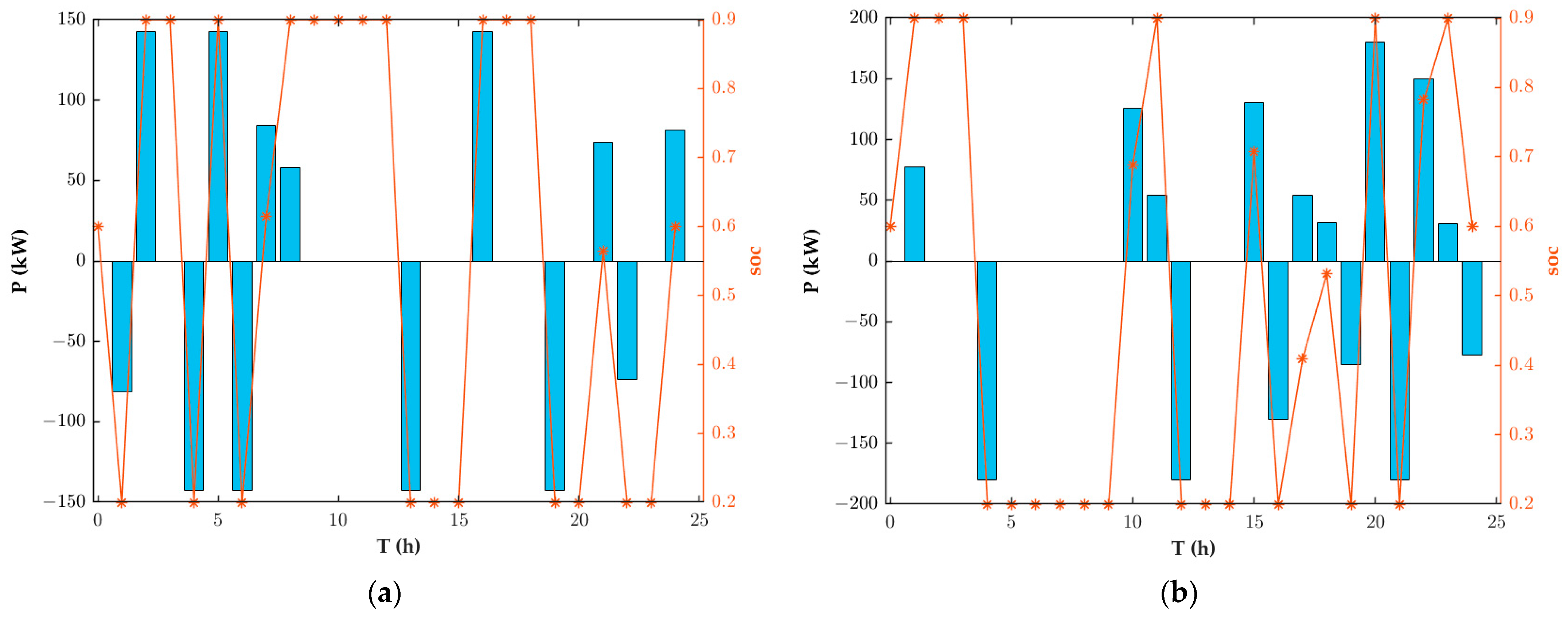
Figure 7 presents the 24 h power and SOC for two energy storage devices. Focusing on the first energy storage device, part (a) of Figure 7 shows the power over 24 h, represented by the blue bar chart. If the power exceeds zero, the energy storage system is in the charging state. Conversely, if it falls below zero, the device is in the discharging state. If the power is zero, neither charging nor discharging occurs. The yellow asterisk represents the SOC of the energy storage device. It is assumed that the energy storage device maintains a balance of charge and discharge during a study cycle, that is, the SOC remains unchanged at the beginning and end of the study. The initial SOC of the energy storage device is set to 0.6. The SOC changes with the charging and discharging behavior of the device.

By observing the load curve and the voltage vulnerability curve, a correlation between them becomes evident. When the load is high, the voltage vulnerability at the nodes increases. If the energy storage devices are connected, it is clear that the voltage vulnerability decreases, indicating an improvement in voltage stability. Figure 8 displays the voltage vulnerability and power loss before and after energy storage devices are integrated into the power grid, respectively. After the energy storage devices are connected, according to Formula (4), the average voltage vulnerability is reduced from 0.3639 to 0.2583, it is significantly reduced by 29%, and the voltage stability is greatly improved. Power loss decreased from 1650 kwh to 1050 kwh, reducing the total power loss by 36%. This shows that more electricity can be utilized efficiently without increasing the total amount of electricity generated, thereby improving the economy of the power grid.

5.2. Mobile Energy Storage Devices

Through the simulation of the stationary energy storage devices, the accuracy and feasibility of the proposed model and method are validated. However, the location and capacity of the energy storage devices remained stationary throughout the day. As a result, there is a period of time when the energy storage devices neither charge nor discharge, resulting in low utilization. By utilizing the mobile energy storage method, their location and capacity can be dynamically adjusted throughout the day. Therefore, according to net load demands, the day is divided into various scenarios, and the mobile energy storage devices are dynamically reconfigured to meet load demands in each scenario.

The net load curve is obtained from Figure 5 and shown in Figure 9. The 24 h day is segmented into three time periods based on the average net load over eight consecutive hours.

Table 2. Time and average load for different scenarios.

Scenario	T (h)	Average Net Load (kW)	Net Load Segments
1	01:00–08:00	1050.87	Low
2	09:00–16:00	1965.62	Flat
3	17:00–24:00	2598.12	Peak

lists the time and average load value of each scenario in detail.

In the three scenarios, the configuration schemes of the mobile energy storage devices are shown in Figure 10. During periods of low load, two energy storage devices are connected at nodes 22 and 26, with a capacity of 167 kWh and 123.6 kWh, respectively. As the load increases, two energy storage devices are connected at nodes 2 and 33, with a capacity of 200 kWh and 172 kWh. In this scenario, the existing devices are insufficient to meet the load demands. Therefore, new energy storage devices are dispatched from the energy storage management center. In the highest load scenario, a larger energy storage capacity is required. Consequently, additional energy storage devices must be deployed to the corresponding locations.

The configuration schemes of energy storage devices in each scenario are summarized in

Table 3. The configuration schemes of energy storage devices in different scenarios.

Scenario	Node	Capacity (kWh)	${\mathit{T}}_{\mathit{u}\mathit{s}\mathit{e}}$ (h)
1	22	167	7
	26	123.6	6
2	2	200	6
	33	172	8
3	16	200	8
	26	200	8
Stationary energy storage device	30	204	13
	32	257	15

. The utilization rate of these devices is calculated using Formula (1). Without altering the location and capacity of the energy storage devices, their utilization rates are 54% and 63%. However, when the devices are dynamically adjusted to adapt to different scenarios, their utilization rates increase to 87.5% and 92%, respectively. This calculation demonstrates that dynamically adjusting the location and capacity of energy storage devices can significantly improve their overall utilization.

In Figure 11, the comparisons of the voltage vulnerability and the power loss between the stationary and mobile energy storage strategies in the three scenarios are proposed. As for voltage vulnerability, it is clear that the mobile energy storage strategy brings about smaller values of voltage vulnerability in the three scenarios in comparison to the stationary energy storage strategy. As for power loss, except for a few cases at 6 h and 13 h, the power loss of the mobile energy storage strategy is slightly larger than that of the stationary energy storage strategy. The mobile energy storage strategy also reduces the power loss produced by the stationary energy storage strategy in general.

To sum up, the application of mobile energy storage devices is effective in enhancing voltage stability, reducing power loss, and increasing utilization. Moreover, the IEEE 33-node system can be changed with actual operational situations to enhance the reliability of the simulation study, and real-world cases will be studied in future research.

6. Conclusions

For the purposes of enhancing the voltage stability and utilization of energy storage devices and reducing power loss, mobile energy storage devices and a configuration method were proposed in this paper as renewable energy generation is connected to the power grid. Firstly, it has been proven that the changes to the location and capacity of the energy storage devices have significant influences on voltage stability and power loss. Secondly, by considering the minimization of power loss, the enhancement of voltage stability, and the improvement of the utilization of energy storage devices as the optimization objectives, a multi-objective optimization model has been constructed, which has been solved by the multi-objective particle swarm optimization (MOPSO) algorithm. By using this method, a simulation analysis has been conducted to examine the advantages of mobile energy storage devices within the power grid over stationary ones. The results have demonstrated that the optimal location and ideal capacity of energy storage devices can be effectively determined while enhancing voltage stability, minimizing power losses, and improving the utilization of these devices.

However, it should be noted that the electricity price during the charging or discharging of the energy storage device is not taken into account in this study. Further optimization of the charging or discharging of the energy storage device, combined with peak and valley electricity prices to improve the economy of the grid, is considered to be a future work. In addition, the deployment of energy storage devices is considered to be an ideal state and not a reality; therefore, according to the power grid and the combination of the road network, the fast and efficient deployment of energy storage is a future research direction. In addition, the typical load, wind power, and photovoltaic curves used as examples in this paper are not universal, and their combination with AI-based forecasting will also be the focus of future research.