Article

Numerical Simulation and Application of Coated Proppant Transport in Hydraulic Fracturing Systems

1
Northwest Sichuan Gas District of Southwest Oil and Gasfield Company, Jiangyou 621741, China
2
State Key Laboratory of Oil and Gas Reservoir Geology and Exploitation, Southwest Petroleum University, Chengdu 610500, China
*
Author to whom correspondence should be addressed.
Processes 2025, 13(4), 1062; https://doi.org/10.3390/pr13041062
Submission received: 18 February 2025 / Revised: 6 March 2025 / Accepted: 31 March 2025 / Published: 2 April 2025
(This article belongs to the Section Chemical Processes and Systems)

Abstract

:
The enhancement of proppant conductivity in shale gas fracturing can be effectively achieved through the implementation of coated proppants. After soaking, non-curable viscous resin-coated proppants exhibit progressive viscosity development and spontaneous agglomeration during the transportation phase. Furthermore, upon fracture closure, the formed proppant agglomerates demonstrate significant stability and do not flow back with the fracturing fluid through the wellbore. While contemporary research has mostly focused on proppant coating methodologies, the transportation process of these proppants remains insufficiently investigated. To fill this knowledge gap, a sophisticated migration two-phase flow coupling model was developed utilizing the computational fluid dynamics–discrete element method (CFD-DEM) approach. This model incorporates the bond contact forces between film-coated proppant particles, accounting for their distinctive cementing characteristics during transport. Through comprehensive numerical simulations, the transport properties of film-coated proppants were systematically analyzed. Field application indicated that compared with conventional continuous sand fracturing, the amount of proppant after treatment with viscous resin film was reduced by 35% and the production was increased by about 25–30%. Additionally, the optimization of the field-scale coated proppant transport processes was achieved through the implementation of a lower fracturing displacement combined with staged sand addition.

1. Introduction

Unconventional oil and gas reservoirs now account for most oil and gas production as conventional oil and gas resources approach a later stage of development [1,2,3]. In the shale gas sector, hydraulic fracturing is employed to enhance the low-permeability properties of unconventional reservoirs to boost the oil and gas well output [4]. Impulse sand fracturing creates discrete layers of proppant within fractures. This method optimizes the proppant distribution, enhances the flow channels, and improves the fracture permeability while reducing the proppant consumption [5]. In the field, proppant placement is typically conducted by co-injecting fibers with pulsed sand. While this method is cost-effective, fiber-bound sand exhibits suboptimal performance. This limitation may lead to proppant backflow issues during post-fracture fluid recovery. To improve and utilize the “bonding” quality of fiber-bound proppants, a novel self-polymerizing treatment has recently been invented. This process involves applying resin chemistry to the surface of proppant particles, enabling self-polymerization during wellbore transport and fracturing. The treated proppants polymerize during transport and form stable sand clusters upon fracture closure, effectively preventing backflow, as shown in Figure 1 [6]. The non-curing viscous resin-coated proppant, a novel fracturing material, gradually develops viscous qualities after soaking and may autonomously aggregate during transit. The clusters have a high degree of stability after the crack is sealed. In addition, the hydrophobic action of the coating layer can lessen the reservoir fluid erosion and fracturing fluid adsorption, helping to maintain both long-term diversion and compressive strength [7].
Currently, numerous scholars have conducted numerical simulations of the movement of proppants during the conventional sand fracturing process for shale gas [8]. Zeng et al. (2016) used the coupled CFD-DEM method to simulate the proppant transport process in a hydraulic fracturing system, which mainly focused on the particle–particle/wall contact damping interaction [9]. Zhang et al. (2017) systematically investigated the transport and placement of multi-sized proppants in fractures in vertical and horizontal wells using a coupled CFD-DEM model [10]. Xu et al. (2022) proposed a method introducing the normal distribution random function into the quartet structure generation set to construct the three-dimensional tortuous fracture networks to study the proppant transport in the tortuous fracture network [11]. However, the transport mechanisms of coated proppants differ from those of conventional fracturing proppants, and the clarity regarding their transport processes and sand placement effectiveness remains insufficient. Since the fracture conductivity is directly influenced by the proppant positioning, further research into the transport processes of coated proppants is essential.
This paper proposes a CFD-DEM-based simulation method for coated proppant transport that accounts for particle adhesion and analyzes the transport stages of coated proppants in fractures. Additionally, this research optimizes the hydraulic fracturing with a field-scale pulsed sand injection technique, providing a basis for the design of operational parameters in shale gas fracturing.

2. Coated Proppant Transport CFD-DEM Mathematics Model

The surface viscous resin will agglomerate under the immersion of the fracturing fluid after the coated proppant is introduced into the formation to generate irregular pillars. In contrast to the fiber activity, softening of the film surface during fracture transit causes particles to aggregate and form pillars. The fluid is viewed as a continuum solved in a Euler mesh when using the CFD-DEM method, and the dispersed phase is viewed as a discrete particle moving according to Newton’s law. This approach can more accurately simulate the particle motion and better characterize the particle contact process when two-phase flow is at work.

2.1. CFD-DEM Mathematical Model

In the Euler framework, the CFD-DEM approach solves fluid motion using the Navier–Stokes control equation, and in the Lagrangian framework, it employs Newton’s second law to monitor each actual particle. The empirical resistance model is used to realize momentum exchange between the fluid and particle phases. The computing data between the two grid systems can be communicated in real time on both values.
The fracture fluid flow’s continuity equation and momentum conservation equation are as follows [12]:
t ρ l ε l + ρ l ε l v l = 0
t ρ l ε l v l + ρ l ε l v l v l = ε l P + ε l τ l ¯ ¯ + ρ l ε l g + S p l
τ l ¯ ¯ = μ l v l + v l T
ε l = 1 i = 1 n V p , i V c e l l
where ε l indicates the dimensionless liquid volume fraction of the fracturing fluid. ρ l is the density of the fracturing fluid. v l is the velocity of the liquid phase. P is the pressure in the flow field. τ l depicts the fluid phase’s stress–strain tensor. μ l is the coefficient of liquid viscosity. g is gravity’s acceleration. S p l is the momentum exchange term between the liquid and particle phases. V p , i represents the volume of particle i and V c e l l is the volume of the local fluid computing unit.
The particle phase’s translational and rotational equations are (5) and (6), respectively [13]:
m p , i d v p , i d t = F d r a g , i + F c + m p , i g
I p , i d w p , i d t = T d r a g , i + T c
where F c denotes the contact force between the proppant particles, m p , i denotes the quality of the proppant, v p , i is the velocity of the proppant, and F d r a g , i denotes the drag force of the liquid phase on the proppant. I p , i represents the moment of inertia of the proppant i, w p , i is the angular velocity, and T d r a g , i is the torque of the liquid phase’s drag force on the proppant i.
The soft ball model is chosen in this study to determine the proppant-to-wall contact. The Hertz–Mindlin (no-slip) contact model and a customized normal cohesive force model are used to determine the normal and tangential forces of particle contact. As a result, it can accurately describe how proppant particles interact to generate irregular pillars. Particle i and particle j produce the following force [14]:
F c , i j = F n , i j + F n , i j d + F t , i j + F t , i j d + F v i s , i j
where F n , i j is the normal force, and F n , i j d is the normal damping force. F t , i j is the tangential force and F t , i j d is the tangential damping force. F v i s , i j is the binding force between particles.
The solvation of the fracturing fluid on the surface resin is crucial for the agglomeration of coated proppants in the formation. The particles undergo water absorption and softening, transitioning from the initial solid condensation state to the coating film viscoelastic state as the fracture fluid permeates into the surface coating resin. The surface resin coating film’s hydration layer exhibits a viscoelastic state with binding properties, which can help the coating film’s proppant particle system maintain the aggregation state. The degree of softening is primarily influenced by three key factors: contact duration, temperature, and pH. Temperature and pH changes are not taken into account in this study; just the change in the contact time is. Changes in the temperature and pH can be studied in subsequent studies. Fu et al. (2016) found the first 10 min after coming into contact with the fracturing fluid are when coated proppant softens the most, after which time it tends to stabilize [15]. By using needle penetration, we can depict the degree of softening, as shown in Figure 2.
Based on the preceding analysis, this study addresses the adhesive characteristics of resin-coated proppants, specifically their agglomeration behavior resulting from the softening of the surface polymer coating upon water contact. An augmented normal contact force model is incorporated into the foundational Hertz–Mindlin (no-slip) contact model to characterize the adhesive interactions between proppant particles. The model assumes uniform and identical adhesive forces among all the coated proppant particles during the transport process. This enhancement enables the CFD-DEM proppant transport model to more accurately simulate the transport and placement patterns influenced by the clustering effects of coated proppants. The normal force model incorporates a penetration degree number into the linear adhesion force model to characterize the contact process between proppant particles. The penetration degree number progressively increases with the contact duration until reaching a stable equilibrium state. Also, we assume that the increase in the adhesion force during softening is proportional to the increase in the penetration, and based on the normal linear spring model, the normal adhesion force between particles is:
F v i s , i j = K π R * δ n 1 4 δ n 2 P P max
K = F v i s max π R max * δ n max 1 4 δ n max 2
where K is the adhesion force per unit area. R * is the equivalent radius of the model particles. δ n is the normal overlap. P is the penetration degree number, which is defined as P = 7.6118 ln ( t ) + 22.435 . P max is the maximum penetration degree. F v i s max is the maximum adhesion force between particles. t is the contact time between the particles and fluid, scaling at the model scale.
In liquid–solid multiphase flow, particles experience various fluid forces. Here, the Gidaspow drag model is used to quantify the drag force caused by the fracturing fluid flowing on the proppant particles:
F d r a g , i = V p β v l v p , i 1 ε l
β = 150 1 ε l 2 μ l d p 2 ε l + 1.75 ρ f 1 ε l v l v p , i d p ε l < 0.8 3 4 C D v l v p , i ρ f 1 ε l d p ε l 1.65 ε l 0.8
C D = 24 1.0 + 0.15 Re 0.687 / Re Re 1000 0.44 Re > 1000
Re = ρ d p v l v p , i ε l μ f
where β is the two-phase exchange coefficient. C D is the particle drag coefficient. d p is the diameter of particle. Re is the Reynolds number.
The force of the particles acting on the fluid, which is identical to the reaction force of the fluid acting on the particle drag force, is the momentum exchange source term of the liquid–solid phase. It may be stated as follows:
S p l = 1 V c e l l i = 1 N F d r a g , i
where N is the total number of proppant particles in the grid, which is dimensionless.

2.2. Model Parameters and Verification

The fracture geometry model is developed based on an established similarity criterion. In the fluid calculation grid, the developed fracture model has to be discretized. Given that the fracture model is represented as a rectangular plate, a regular hexahedral grid structure can be employed to achieve effective control of the volume discretization. The rectangular fracture model developed in this study has dimensions of 300 mm, 60 mm, and 2 mm, which are comparable to the Reynolds number of the formation fractures. In addition, the grid independence of the fluid computing grid in the model is verified, and it is found that the addition of the grid has little effect on the calculation results when the dimensions in the x, y and z directions reach 3 mm, 2 mm and 1 mm, respectively. Figure 3 shows the height flow velocity at length x = 150 mm under different grid numbers. The DEM computational grid is three times the particle mode’s radius. The fracture fluid and proppant particles enter the model through the inlet, which is located at the left border and is designated as the velocity inlet boundary. The outlet, which is the constant pressure barrier, is then placed at the right end. While the particle wall is thought of as a discrete element particle contact model, the liquid wall boundary is a non-slip barrier. Table 1 lists several simulation parameters, including the Young’s modulus and Poisson’s ratio. The fluid phase control equation is discretized using the first-order upwind strategy for the CFD-DEM coupling model’s solution, the discrete equation is iteratively computed using the SIMPLE algorithm, and the particle phase is iteratively calculated using the Euler display difference method. The CFD time step in the coupling calculation is 3 × 10⁻⁴ s, while the DEM time step is 3 × 10⁻⁶ s.
The channel fracture sand dispersion experiment was contrasted with the simulation of a sandbank in order to verify the CFD-DEM coupling approach. Figure 4 depicts the ultimate sandbank form based on the viscosity of 40 mPas and the displacement of 4.8 m3/h, comparing the distribution law of the Qingzhi’s [16] plate transport physical model experiment on the channel-fracturing sand beach. Similar to the experiment, the same factors are used to determine the form of a sand dike in addition to its total size. There are fewer channels than at the outflow because the sand dike at the entry is taller and the pillars there have been compressed by the fluid’s scour. It is shown that the CFD-DEM coupling model with the additional adhesive contact force of coated proppant particles can better simulate the transportation and placement process of coated proppant.

3. Numerical Simulation Results and Applications

This section first discusses the characteristics of the coating proppant transport process and then applies it to the actual parameters of fracturing in well X.

3.1. Transport Characteristics

Through simulation analysis, we identified four distinct stages in terms of coated proppant transport over a 5 s duration. During the initial injection phase, known as the proppant contact softening stage, the film proppant’s surface has not fully softened, resulting in weak surface adhesion forces that prevent pillar formation under fluid drag conditions. At this point, a layer of sand dunes is being generated by sedimentation, the flow rate is downhill, and the proppant is being impacted by gravity in a vertical direction. As illustrated in Figure 5a, the unsettled proppants continue to migrate away from the viscous resistance.
The proppant particles continue to soften throughout the contact process as the contact time increases. The two particles are joined together when their adhesive forces are equivalent to the combined forces of gravity and fluid drag. The sandbank begins to steadily increase at 1.2 s, as illustrated in Figure 5b. The injectable proppant initially generates agglomerates, which then gradually settle and aggregate as a result of their adhesive interaction. Figure 6 shows the flow of the proppant cluster in the fracture of the slab. This phase, characterized by the development of proppant pillars, is known as the proppant agglomeration paving stage.
The proppant aggregates on the surface to form a sandbank with pillars as the injection time goes up, intensifying the effect of proppant agglomeration. The proppant sandbank progressively accumulates and expands along the fracture’s height. In order to allow the unsettled proppant particles to go farther and form pillars and settle, the flow section on the upper half of the sandbank gradually shrinks as the sandbank expands. Between 1.2 and 2.5 s, high-velocity fluid flow causes fluidization of the settled proppant pillars as the sandbank elevates. The particles are detached from the pillar when the drag force outweighs the combined force of adhesion and gravity. The placement stage of the proppant pillars along the fracture height occurs when the force returns to equilibrium and the particles aggregate and move to a new location.
Once the sandbank created by the proppant pillars reaches a critical height at the fracture front, its upward movement ceases. At this point, increased flow rates result in accelerated scouring of the settled pillars by high-velocity fracturing fluid. The sandbank height stabilizes when the settlement of the pillars on it reaches equilibrium with the quantity of particle scour during fluidization, indicating that it has reached a balance height. Additionally, the proppant pillars are transported forward until they are evenly distributed throughout the fracture before being delivered to the ends of the fracture through the flow section at the top of the fracture.

3.2. Parametric Studies

The injection flow rate significantly influences the proppant transport velocity and pillar formation patterns in channel fracturing. Numerical simulations were conducted under the following conditions: injection velocities ranging from 0.20 to 0.35 m/s (at 0.05 m/s intervals), fracturing fluid viscosity of 20 mPa·s, proppant concentration of 8%, particle diameter of 0.4 mm, and proppant density of 2200 kg/m3.
In this paper, the pore volume ratio is calculated by Formula (15):
C = V h V t = 1 V P V t × 1 ε
V t = x = g L g R l H w
where C is the pore volume ratio. V h is the pore volume. V t is the total volume of the sandbank. V p is the volume of particles. ε is the porosity of the particles during accumulation, and the value is 0.6. gL and gR are the left and right boundary grids of the sandbank, respectively. l is the grid length, and the value is 3. H is the height of the sandbank boundary grid to the bottom. w is the fracture width, namely 2 mm.
As seen in Figure 7, as the injection rate is increased, the pore volume ratio first rises and subsequently falls. As a result, channel fracturing is not ideal for large pumping rates, and the operator must optimize the pumping rates in accordance with the field circumstances.
The effects of the fracturing fluid viscosity on the coated proppant transport dynamics and sandbank formation are also discussed. Simulations were performed using constant parameters (flow velocity: 0.269 m/s, field rate: 5 m3/min, proppant concentration: 4%, particle diameter: 0.4 mm, density: 2100 kg/m3) while varying the fluid viscosities (10–60 mPa·s) to assess their impact on the proppant placement efficiency and channel development.
Figure 8 illustrates the relationship between the fracturing fluid viscosity and the sandbank pore volume ratio. The data demonstrate a positive correlation between the fluid viscosity and the pore volume ratio, attributable to the enhanced proppant transport capacity at higher viscosities. This suggests that strategic optimization of the fracturing fluid viscosity can improve the transport efficiency and pore volume development.

3.3. Field Application

Well X is a horizontal well situated in the Sichuan northwest field. With a horizontal section of 1500 m, the well was drilled to a depth of 5230 m. The well was completed in the Longmaxi Formation using a 139.7 mm casing. Gas logging revealed high-quality hydrocarbons.
Modeling was based on the actual situation on-site. A pump injection rate of 12 m3/min was selected to add the liquid. High-viscosity fracturing fluid was also used, and proppant was introduced in batches. According to the simulation of the proppant delivery, a uniform sand-laying effect can be obtained.
Proppant pulse injection enhances proppant transport efficiency and promotes large-scale pillar formation through injecting a pure liquid section into the injection gap in a sand mixture. The following simulation parameters were applied: injection flow rate of 0.27 m/s, fracturing fluid viscosity of 20 mPa, proppant concentration of 8%, particle size of 0.4 mm, and density of 2200 kg/m3. As demonstrated in Figure 9, the pore volume ratio of the sandbank initially increases and subsequently declines as the pulse injection interval duration increases. Proppant pillars are distributed and better channels can form between the small, settled pillars when the gap period is appropriate. Insufficient intervals will lead to channel compression, which will increase the fracturing fluid’s displacement effect on the mixture. Conversely, excessive pulse intervals will result in large proppant pillars settling too fast, the proppant pillars’ growth along the fracture height stage will be too short, and the pore volume ratio will be reduced. The simulation results are converted to the field time by the similarity criterion, and the best results are obtained with pulse intervals of 2–3 s.
According to the data in the field, the amount of self-aggregating proppant after being covered in a viscous resin film was reduced by 35% when compared to conventional fracturing, and the real-time data of the fracturing revealed that the concentration of proppant slug increased quickly during the pulse sanding process without delay phenomenon, allowing the ground control system to successfully open and close the valve, as shown in Figure 10. Proppant particles may self-assemble into “sand clusters” during transit when viscous resin is present. They can also easily flow through perforation holes and be injected into fractures to create highly conductive fracture channels. Also, compared to untreated adjacent wells, the production has increased by about 25–30%. At the same time, the fracturing fluid is also saved, and the amount of proppant flowback is reduced.

4. Conclusions

(1)
The two-phase flow coupling model based on the CFD-DEM approach taking into account the adhesive contact of coated proppant particles can better simulate the transport process of coated proppant in the fracture thanks to prior data and experimental verification.
(2)
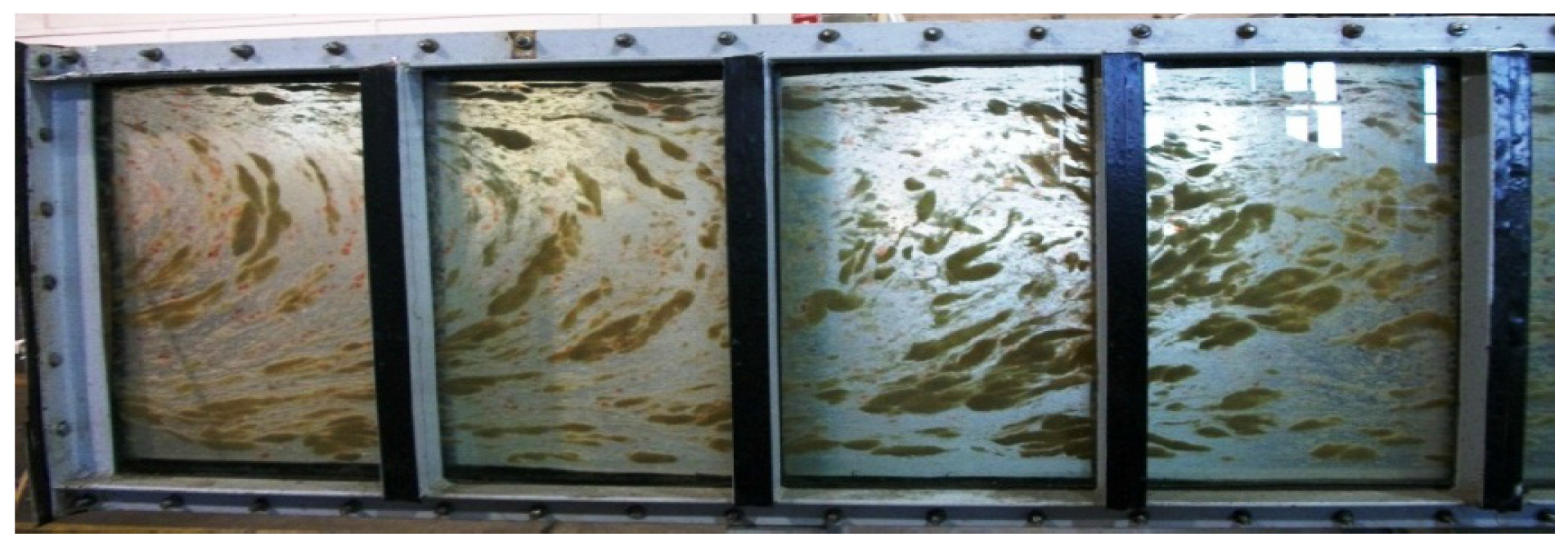
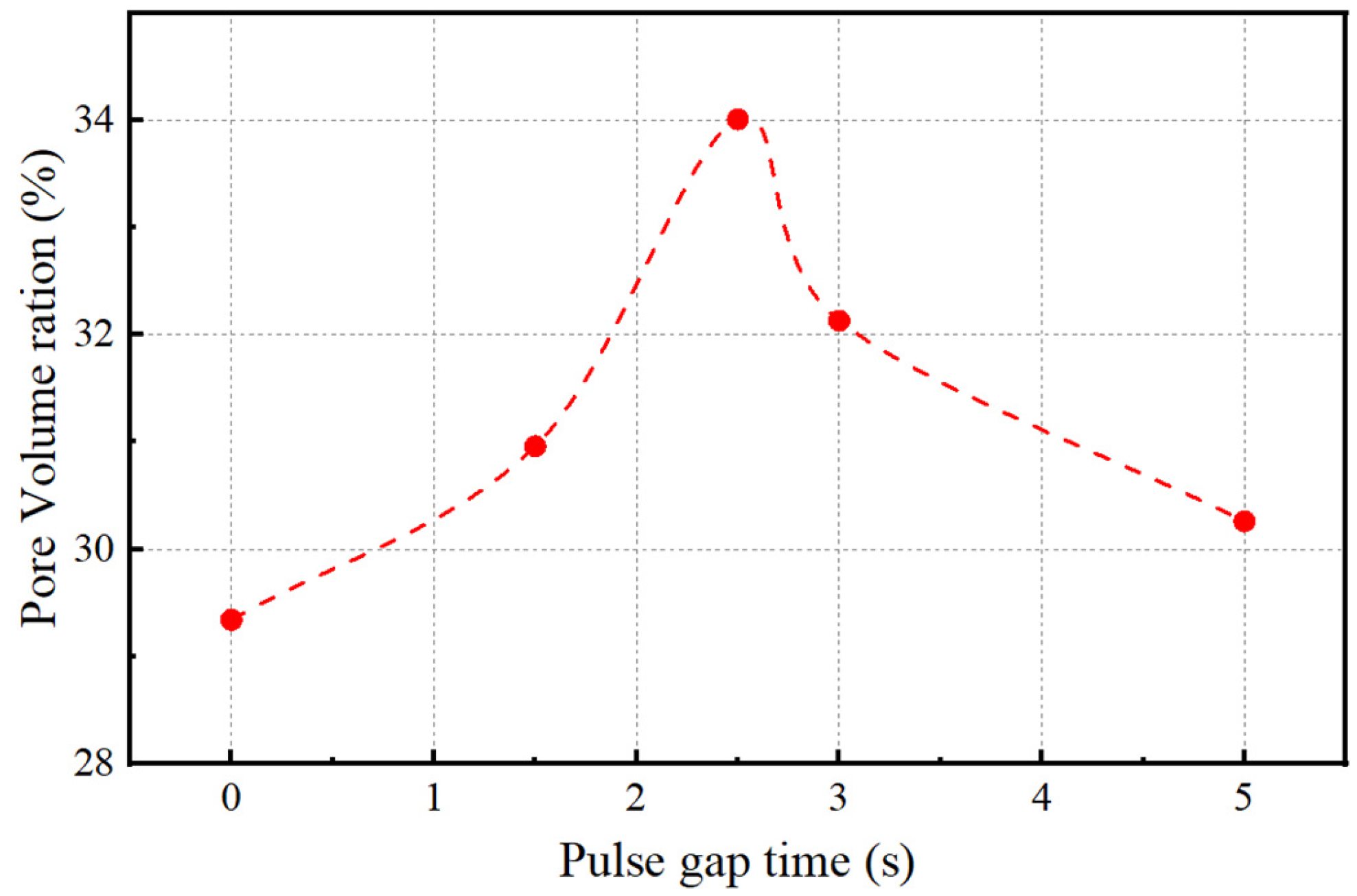
The four stages of transportation in plane vertical cracks are separated by dynamic changes in the coated film proppant particles generating pillars. (1) The softening of proppant particles upon contact with fluid; (2) the positioning of the proppant pillars along the fracture height; and (3) the placement of the proppant pillars along the fracture length. The pore volume ratio can be raised by shortening the fourth stage time.
(3)
Field results show that compared with conventional continuous sand fracturing, the amount of proppant after treatment with viscous resin film is reduced by 35%, and the proppant particles can self-aggregate during transportation to form “sand clusters” to form highly conductive fracture channels.

Author Contributions

Methodology, Q.D.; writing—original draft, H.Y. (Hua Yang) and S.H.; writing—review and editing, P.D.; investigation, X.Y.; software, C.L.; validation, Z.S.; supervision, L.R.; funding acquisition, H.Y. (Hanxiang Yin); project administration, B.H.; resources, R.L. All authors have read and agreed to the published version of the manuscript.

Funding

This research was funded by the National Natural Science Foundation of China, grant number U21B2071; National Natural Science Foundation of China, grant number 52104038; National Natural Science Foundation of China, grant number 52104039; and Science and Technology Cooperation Project of the CNPC-SWPU Innovation Alliance, grant number 2020CX030201.

Data Availability Statement

The original contributions presented in this study are included in the article. Further inquiries can be directed to the corresponding author.

Acknowledgments

Thank you to the Southwest Oil and Gas Field Company and Southwest Petroleum University for their strong support of this research.

Conflicts of Interest

Authors Qiang Du, Hua Yang, Shipeng He, Xun Yang, Xun Yang, Zhiyun Sun, Hanxiang Yin and Bencheng He was employed by the company Northwest Sichuan Gas District of Southwest Oil and Gasfield Company. The remaining authors declare that the research was conducted in the absence of any commercial or financial relationships that could be construed as a potential conflict of interest.

References

  1. Chen, J.; Cao, J.; Han, H.; Nian, J.; Guo, L. Adaptability Analysis of Commonly Used Production Prediction Models for Shale Oil and Gas Wells. Unconv. Oil Gas Resour. 2019, 6, 48–57. [Google Scholar]
  2. Lin, H.; Deng, J.; Xie, T.; Huo, H.; Chen, Z. Effect of Formation Anisotropy on Wellbore Stability of Hard Brittle Shale. J. Northeast. Pet. Univ. 2021, 45, 85–94. [Google Scholar]
  3. Wang, H.; Feng, M.A.; Tong, X.; Liu, Z.; Zhang, X.; Wu, Z.; Li, D.; Wang, B.; Xie, Y.; Yang, L. Assessment of Global Unconventional Oil and Gas Resources. Pet. Explor. Dev. 2016, 43, 925–940. [Google Scholar]
  4. Zhao, J.; Zhao, X.; Zhao, J.; Cao, L.; Hu, Y.; Liu, X. Coupled Model for Simulating Proppant Distribution in Extending Fracture. Eng. Fract. Mech. 2021, 253, 107865. [Google Scholar]
  5. Qian, B.; Yin, C.; Zhu, J.; Chen, X. Research and Practice of the Impulse Sand Fracturing Technology. Nat. Gas Ind. B 2015, 2, 334–340. [Google Scholar] [CrossRef]
  6. Inyang, U.A.; Nguyen, P.D.; Cortez, J. Development and Field Applications of Highly Conductive Proppant-Free Channel Fracturing Method. In Proceedings of the SPE Unconventional Resources Conference/Gas Technology Symposium, The Woodlands, TX, USA, 1–3 April 2014; SPE: Richardson, TX, USA, 2014; p. D031S006R006. [Google Scholar]
  7. McDaniel, B.W.; Weaver, J.D. Fracture Stimulate and Effectively Prop Fracs: The Conductivity Challenges of Liquids Production from Ultralow-Permeability Formations. In Proceedings of the SPE Canadian Unconventional Resources Conference, Calgary, AB, Canada, 30 October–1 November 2012. [Google Scholar]
  8. Sahai, R.; Moghanloo, R.G. Proppant Transport in Complex Fracture Networks–A Review. J. Pet. Sci. Eng. 2019, 182, 106199. [Google Scholar] [CrossRef]
  9. Zeng, J.; Li, H.; Zhang, D. Numerical Simulation of Proppant Transport in Hydraulic Fracture with the Upscaling CFD-DEM Method. J. Nat. Gas Sci. Eng. 2016, 33, 264–277. [Google Scholar] [CrossRef]
  10. Zhang, G.; Li, M.; Gutierrez, M. Simulation of the Transport and Placement of Multi-Sized Proppant in Hydraulic Fractures Using a Coupled CFD-DEM Approach. Adv. Powder Technol. 2017, 28, 1704–1718. [Google Scholar] [CrossRef]
  11. Xu, J.; Gao, R.; Yang, L.; Liu, Z.; Ding, Y.; Wang, Z.; Mo, S. A 3D Tortuous Fracture Network Construction Approach to Analyze Proppant Distribution in Post-Fractured Shale. J. Pet. Sci. Eng. 2022, 208, 109676. [Google Scholar] [CrossRef]
  12. Akhshik, S.; Rajabi, M. Simulation of Proppant Transport at Intersection of Hydraulic Fracture and Natural Fracture of Wellbores Using CFD-DEM. Particuology 2022, 63, 112–124. [Google Scholar] [CrossRef]
  13. Zhao, J.; Shan, T. Coupled CFD–DEM Simulation of Fluid–Particle Interaction in Geomechanics. Powder Technol. 2013, 239, 248–258. [Google Scholar] [CrossRef]
  14. Ren, L.; Lin, C.; Zhao, J.; Lin, R.; Wu, J.; Wu, J.; Hu, Z. Numerical Simulation of Coated Proppant Transport and Placement in Hydraulic Fractures Based on CFD-DEM. Pet. Sci. Technol. 2024, 42, 3334–3354. [Google Scholar] [CrossRef]
  15. Fu, L.; Zhang, G.; Ge, J.; Liao, K.; Jiang, P.; Pei, H.; Li, X. Surface Modified Proppants Used for Porppant Flowback Control in Hydraulic Fracturing. Colloids Surf. A Physicochem. Eng. Asp. 2016, 507, 18–25. [Google Scholar] [CrossRef]
  16. Wen, Q.; Yang, Y.; Wang, F. Experimental Study on an Innovative Proppant Placement Method for Channel Fracturing Technique. J. China Univ. Pet. Ed. Nat. Sci. 2016, 40, 112–117. [Google Scholar]
Figure 1. Proppant “clumps” formed by pulsed sand addition in a flat plate model [6].
Processes 13 01062 g001
Figure 2. The effect of time on the needle penetration.
Processes 13 01062 g002
Figure 3. Grid independence verification (height flow velocity at length x = 150 mm under different grids).
Processes 13 01062 g003
Figure 4. During settlement, a comparison of the proppant pillars’ distribution in the slot.
Processes 13 01062 g004
Figure 5. Coated proppant particle transport process. Figure (ad) are the simulation results for transport stages 1~4, respectively.
Processes 13 01062 g005
Figure 6. Distribution of coated proppant in the slab fracture [6].
Processes 13 01062 g006
Figure 7. Pore volume ratio of the sandbank under different injection flow rates at the final time.
Processes 13 01062 g007
Figure 8. Pore volume ratio of the sandbank under different fracturing fluid viscosities at the final time.
Processes 13 01062 g008
Figure 9. Pore volume ratio of the sandbank under different pulse gap times at the final time.
Processes 13 01062 g009
Figure 10. On-site fracturing construction curve in the oil field.
Processes 13 01062 g010
Table 1. Numerical simulation calculation parameters [14].
ParametersSymbolUnitValues
Domain size-mm300 × 60 × 2
CFD mesh size-mm3 × 2 × 1
Proppant:
Shear modulusEpMPa1 × 102
Poisson’s ratiovp-0.25
Fractured model:
Shear modulusEpMPa7.85 × 103
Poisson’s ratiovp-0.12
Proppant–proppant contact:
Restitution coefficiente1-0.3
Static friction coefficient:μs1-0.5
Rolling friction coefficient:μr2-0.1
Proppant–fractured contact:
Restitution coefficiente2-0.24
Static friction coefficient:μs2-0.194
Rolling friction coefficient:μr2-0.005
Disclaimer/Publisher’s Note: The statements, opinions and data contained in all publications are solely those of the individual author(s) and contributor(s) and not of MDPI and/or the editor(s). MDPI and/or the editor(s) disclaim responsibility for any injury to people or property resulting from any ideas, methods, instructions or products referred to in the content.

