Article

Research on the Prediction of Cement Precalciner Outlet Temperature Based on a TCN-BiLSTM Hybrid Neural Network

College of Materials Science and Engineering, Nanjing Tech University, Nanjing 211816, China
*
Author to whom correspondence should be addressed.
Processes 2025, 13(12), 4068; https://doi.org/10.3390/pr13124068
Submission received: 20 November 2025 / Revised: 10 December 2025 / Accepted: 11 December 2025 / Published: 16 December 2025
(This article belongs to the Section Chemical Processes and Systems)

Abstract

As the global cement industry moves toward energy efficiency and intelligent manufacturing, refined control of key processes like precalciner outlet temperature is critical for improving energy use and product quality. The precalciner’s outlet temperature directly affects clinker calcination quality and heat consumption, so developing a high-accuracy prediction model is essential to shift from empirical to intelligent control. This study proposes a TCN-BiLSTM hybrid neural network model for the accurate prediction and regulation of the outlet temperature of the decomposition furnace. Based on actual operational data from a cement plant in Guangxi, the Spearman correlation coefficient method is employed to select feature variables significantly correlated with the outlet temperature, including kiln rotation speed, high-temperature fan speed, temperature A at the middle-lower part of the decomposition furnace, temperature B of the discharge from the five-stage cyclone, exhaust fan speed, and tertiary air temperature of the decomposition furnace. This method effectively reduces feature dimensionality while enhancing the prediction accuracy of the model. All selected feature variables are normalized and used as input data for the model. Finally, comparative experiments with RNN, LSTM, BiLSTM, TCN, and TCN-LSTM models are performed. The experimental results indicate that the TCN-BiLSTM model achieves the best performance across major evaluation metrics, with a Mean Relative Error (MRE) as low as 0.91%, representing an average reduction of over 1.1% compared to other benchmark models, thereby demonstrating the highest prediction accuracy and robustness. This approach provides high-quality predictive inputs for constructing intelligent control systems, thereby facilitating the advancement of cement production toward intelligent, green, and high-efficiency development.

1. Introduction

The outlet temperature of the decomposition furnace serves as a critical indicator of the thermal stability of the pre-calciner system, directly determining the efficiency of raw meal decomposition, the final quality of clinker, and the economic performance of system operation [1]. From the perspectives of process mechanism and control, this temperature is influenced by the strong coupling of multiple variables. Specifically, for the production line on which this study is based, the key measurable and controllable variables affecting the outlet temperature mainly include driving and conveying parameters, such as kiln speed and high-temperature fan speed, which collectively determine the residence time and flow state of materials and gases within the system; key temperature parameters at specific locations, such as the temperature at the middle-lower part of the decomposition furnace and the discharge temperature from the five-stage cyclone, which directly reflect the heat distribution and heat exchange progress in the system; gas flow control and air temperature parameters, such as exhaust fan speed and tertiary air temperature of the decomposition furnace, which regulate the oxygen content and total enthalpy input of the system. Together, these variables constitute a complex thermal system characterized by highly nonlinear and significantly delayed dynamics.
When the outlet temperature of the precalciner is too low, it may result in a decomposition rate of CaCO3 in the raw meal falling below 85%, causing a large amount of undecomposed material to enter the rotary kiln. This leads to the free calcium oxide (f-CaO) content exceeding 2%, which in turn causes volumetric expansion and cracking during the later stages. Moreover, inadequate temperature can lead to incomplete combustion of pulverized coal, with CO concentration rising from 50 ppm to over 200 ppm, necessitating additional ammonia injection for treatment [2]. On the other hand, if the temperature is excessively high, it may disrupt the thermal balance of the downstream process system, increase the heat consumption of the sintering process, and consequently affect the overall stability of the sintering system [3]. Therefore, constructing a high-precision prediction model based on the aforementioned key variables holds critical engineering significance for achieving precise feedforward control of the outlet temperature, ensuring stable product quality, and reducing coal consumption and emissions.
In recent years, deep sequential models such as Temporal Convolutional Networks (TCN) [4], bidirectional recurrent networks [5], and attention mechanisms [6] have emerged as mainstream paradigms in the field of time series forecasting internationally. In the field of temperature prediction, Rahman et al. [7] utilized multi-source time series data such as raw meal feed rate, temperatures at various levels, pressures, and gas compositions as inputs to predict the outlet temperature of the decomposition furnace. The constructed CNN-LSTM-Attention hybrid model demonstrated high accuracy, but its performance heavily relied on the stable allocation of attention weights. Similarly, Sun et al. [8] used inputs such as kiln torque, kiln outlet temperature, and exhaust gas composition to predict the burning zone temperature of the rotary kiln. Their proposed Hammerstein model combining CNN-GRU-Attention with ARX enhanced interpretability but remained insufficient in modeling the dynamics of strongly nonlinear systems. Raza [9] directly modeled temperature series using multivariate CNN with attention mechanisms, with input variables similar to those in Rahman et al.’s study. However, the model complexity and its robustness to sudden operational changes were inadequate. In energy consumption and emission prediction, Liu et al. [10] employed motor current, material flow rate, and other inputs to predict the power consumption of the cement raw mill system. The LSTM-with-spatial-attention-mechanism model they used was effective but limited in generalizing to different process stages. Okoji et al. [11] used combustion parameters and operational variables as inputs to predict NOx emissions. Their method, combining adaptive neural networks with genetic algorithms, improved adaptability but was constrained by computational efficiency for real-time applications. In system modeling and control, Li et al. [12] focused on the lime rotary kiln, using various temperature, pressure, and flow signals as inputs to predict key internal temperatures. Their CNN-BiLSTM-OC model reduced errors by analyzing system inertia and time delays, but its applicability to cement pre-calciner systems remains unverified. Yang et al. [13] and Wang et al. [14] modeled cement rotary kilns using BP, Elman, and RNN attention networks, respectively, with inputs mostly comprising traditional process variables. Although progress was made in short-term prediction, these models generally suffered from limited generalization capabilities. Ali et al. [15] and Santos et al. [16] focused on waste heat power generation prediction (using inputs such as steam parameters) and kiln temperature control (using state variables as inputs), respectively. The former simplified thermodynamic calculations, while the latter faced deployment bottlenecks due to high computational resource consumption. In summary, existing research often relies on empirical approaches for feature selection, lacking a transparent screening framework. While model architectures have become increasingly complex, their ability to synergistically model local features and long-term dependencies, as well as their robustness under varying operating conditions, remains inadequate. These are also common challenges faced by the international industrial forecasting community [17]. To address these issues, this study proposes a prediction framework that integrates Temporal Convolutional Networks (TCN) with causally constrained Bidirectional Long Short-Term Memory (BiLSTM), aiming to enhance the model’s representational capacity and causal robustness. This effort responds to the ongoing demand within the international academic community for interpretable and robust industrial forecasting models.
The paper proposes an innovative framework that integrates classical statistical learning with deep learning. First, the Spearman rank correlation coefficient is introduced to perform interpretable feature screening, identifying key variables such as kiln speed and high-temperature fan speed, thereby addressing issues of input redundancy and ambiguous physical significance. To overcome the limitations of classical methods in modeling complex nonlinear time series, a TCN-BiLSTM hybrid model is further proposed. This model combines the local feature extraction capability of temporal convolutional networks with the long-term dependency modeling ability of causally constrained bidirectional long short-term memory networks, deeply uncovering the complex dynamics of key variables. This framework systematically integrates interpretable feature engineering with powerful time-series modeling, providing an accurate, robust, and interpretable solution for predicting critical industrial parameters.

2. Process Description and Variable Selection

2.1. The Precalciner Kiln Process

The precalciner kiln is the core process of modern new dry-process cement production. By transferring the carbonate decomposition stage from the rotary kiln to the decomposition furnace, it significantly enhances production efficiency and energy utilization [18]. As shown in Figure 1, the precalciner kiln production process consists of five key stages: raw material processing, preheating, decomposition, calcination, and cooling. The core equipment in each stage directly or indirectly affects the outlet temperature of the decomposition furnace. During raw material processing, crushers, batching scales, and ball mills are employed. Improper raw material particle size or formulation can reduce preheating and decomposition efficiency, leading to fluctuations in the decomposition furnace outlet temperature [19]. The multi-stage cyclone preheater utilizes exhaust gas from the rotary kiln to preheat raw meal. If seal failure causes gas leakage, insufficient preheating of the raw meal occurs, requiring additional heating in the decomposition furnace thereby driving up its outlet temperature [20].
One of the core control objectives in the production process of a precalciner kiln is achieving precise regulation of the temperature at the outlet of the decomposition furnace. The TCN-BiLSTM hybrid neural network, leveraging its capability for in-depth mining of multi-dimensional time-series data and dynamic modeling, provides an efficient solution to this challenge. On one hand, it effectively mitigates issues such as unstable clinker quality and surging fuel consumption caused by temperature anomalies. On the other hand, by proactively predicting temperature trends, it significantly enhances production efficiency, reduces overall energy consumption, and facilitates the intelligent and green transformation of the cement industry.

2.2. Variable Screening Using Spearman’s Rank Correlation

In the modeling and optimization research of precalciner outlet temperature, the scientific and rational selection of characteristic variables is a key prerequisite for ensuring the predictive accuracy of the model. In this paper, the Spearman rank correlation coefficient method is used to select and validate the original characteristic variables. The Spearman rank correlation coefficient performs linear correlation analysis based on the rank order between two variables [21]. The formula for calculating the SR correlation coefficient is:
ρ = 1 6 i = 1 n d i 2 n ( n 2 1 )
where d i represents the rank difference between the two data variables, ρ is the SR correlation coefficient bounded by −1 ≤ ρ ≤ 1 (Equation (1)). n is the number of data samples. Based on the absolute value of the correlation coefficient derived from this method, the correlation strength can be roughly categorized as follows: no correlation (0~0.1), weak correlation (0.1~0.3), moderate correlation (0.3~0.8), and strong correlation (0.8~1). In general, when the absolute value of the correlation coefficient exceeds 0.3, the variable can be used as a predictive characteristic variable [22]. After obtaining the data from the cement plant, preprocessing is carried out to remove outliers and missing values, and the correlation coefficients between the characteristic variables and the precalciner outlet temperature are computed.
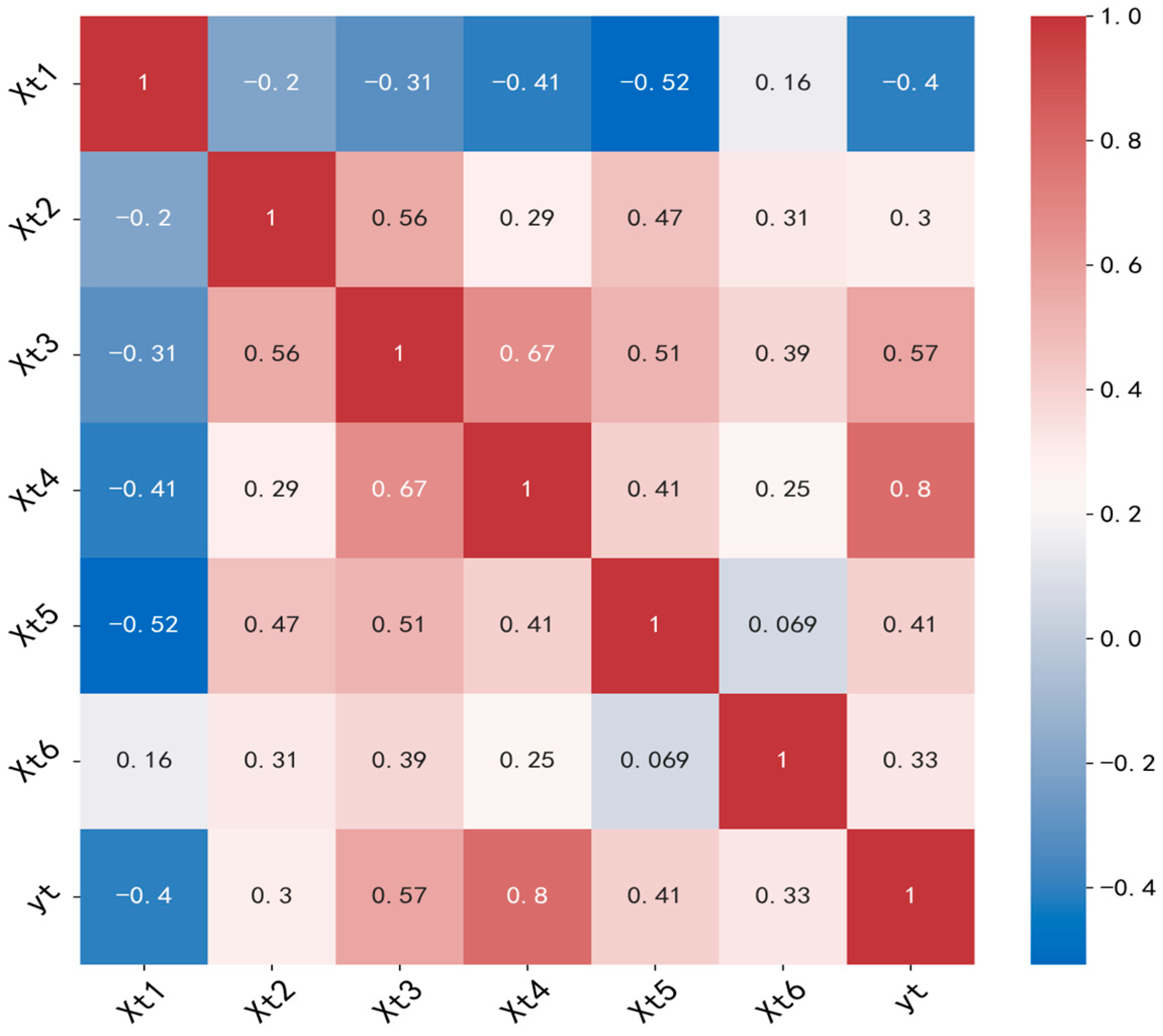
The dataset is collected from the Distributed Control System (DCS) and thermal sensors of a cement plant in Guangxi, China, covering continuous records of four months of normal operation. This study employs the Spearman rank correlation coefficient to screen process variables that exhibit statistically significant correlations with the outlet temperature of the decomposition furnace. Six key operational parameters are ultimately identified as model inputs, with the outlet temperature itself serving as the output target. Detailed descriptions of each variable, including variable labels, physical meanings, symbols, and units, are summarized in Table 1. As can be seen from Figure 2, Yt serves as the key response variable in this study for characterizing the thermal state of the combustion system, which serves as the key response variable characterizing the thermal state of the combustion system in this study. Notably, Xt4 exhibits the most similar fluctuation pattern and strongest influence on the calciner outlet temperature, with their correlation coefficient reaching 0.8. This is because, in actual production, if the material feeding temperature is too high or too low, the decomposition rate of the raw meal will deviate from the target (generally required to be ≥90%), which in turn leads to a rise or fall in the precalciner outlet temperature. The coefficient value of Xt3 at 0.57 indicates a moderate correlation. This is because zone A in the lower-middle temperature region serves as the primary combustion zone of the fuel, reflecting the intensity of fuel combustion and directly driving changes in the outlet temperature. The fluctuations of Xt1 and Xt5 are the most similar, with coefficient values of 0.4 and 0.41, respectively. Xt2 and Xt6 have coefficients of 0.3 and 0.33. All four influencing factors exhibit moderate correlations. It can thus be concluded that the rank correlation coefficient is beneficial in capturing nonlinear relationships and in mitigating the impact of noise on model performance.

2.3. Sensitivity Analysis

Building upon the Spearman correlation analysis for variable screening, perturbation-based sensitivity analysis was employed to quantify the relative importance of each input variable in the TCN-BiLSTM model. A ±5% perturbation was applied to each variable to calculate the average change in the outlet temperature of the precalciner. As shown in Figure 3, the discharge temperature of the fifth-stage cyclone B consistently emerged as the primary influencing factor in both analyses. The tertiary air temperature exhibited a significant increase in importance, rising from the 5th to the 2nd position, indicating that the model effectively captured its nonlinear interactive effects. Conversely, the relative importance of kiln speed and the mid-lower temperature of precalciner A decreased, reflecting the model’s automatic optimization in handling multicollinear features. This analysis validates the physical rationality of the model’s decision-making and demonstrates the capability of deep learning to uncover complex underlying relationships within industrial data.

3. TCN-BiLSTM Model Construction

3.1. Residual Blocks and Causal Dilated Convolution

Temporal Convolutional Network (TCN) is a convolutional architecture designed for sequence modeling, aiming to address the limitations inherent in recurrent neural networks. It is often used for mining image information and predicting sequential data. Compared with typical recurrent networks, the TCN architecture is simpler and clearer, mainly composed of residual modules and causal convolutions [23].
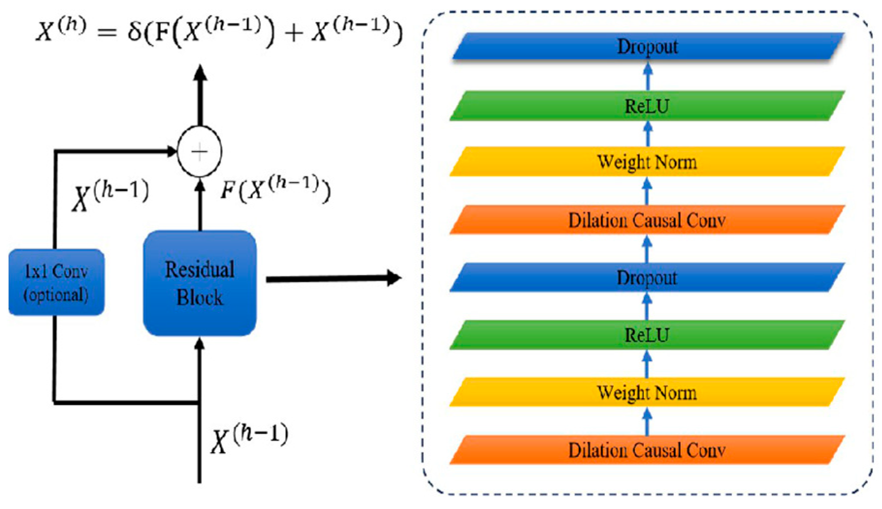
To enhance network depth and improve the ability to model complex temporal dependencies, TCN adopts residual blocks as its basic building units. Each residual unit is a small neural network with a residual connection. The use of residual connections accelerates feedback and convergence in deeper networks, resolving the degradation problem caused by increasing network layers. Each residual unit contains two convolutional units and a 1 × 1 convolution layer. The convolution units achieve a larger receptive field by adjusting the dilation rate, thereby enabling the network to retain sufficiently long-term information. Moreover, they only convolve the input data prior to the target time t to generate the output at time t, ensuring no information leakage occurs. Then, the weights are normalized, and the ReLU function is used as the activation function. Finally, a Dropout operation is applied to randomly discard certain neurons to accelerate model training and prevent overfitting [24]. As shown in Figure 4, the output of the h-th residual module F( X ( h 1 ) )is added to the input X ( h 1 ) to obtain the new input x ( h ) :
X ( h ) = δ ( F X h 1 + X h 1 )
where δ denotes the activation function.
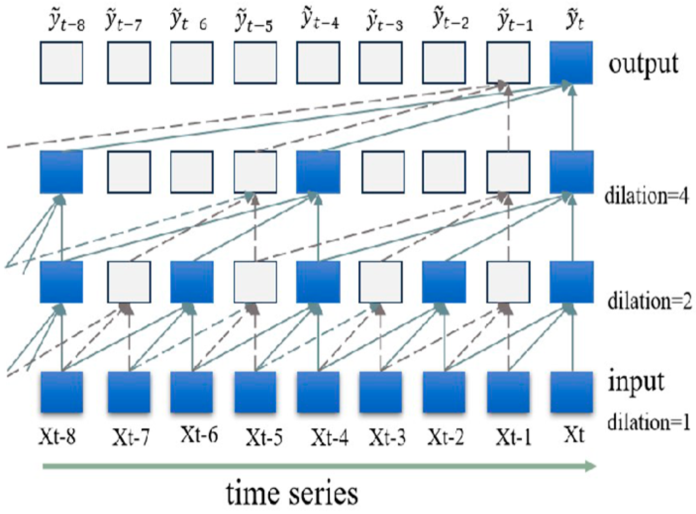
The convolution operation used in the residual block is causal convolution, whose core purpose is to ensure that the model output depends solely on the current and past input data, thus strictly adhering to temporal causality [25]. As shown in Figure 5, causal convolution can be understood as a one-way transmission of temporal data. Unlike traditional convolutional neural networks, causal convolution prohibits future data from influencing the past, and convolution operations can only be performed on the current and preceding time steps [26]. Dilated convolution enlarges the receptive field by inserting convolution kernels with specific spacing, where the interval size is defined by the dilation rate. The dilation rate is expressed as [d1, d2, d3,…] = [ 2 0 , 2 1 , 2 2 ,…]. The formula for dilated convolution is as follows:
F s = X × d f s = i = 0 k 1 f ( i ) · X s d · i
In this equation, X represents the input sequence, f = ( f 1 , f 2 ,…, f k ) represents the input sequence, k is the filter size, d is the dilation factor, and sd · i denotes the past time direction.

3.2. BiLSTM and TCN-BiLSTM

TCN possesses strong parallelism and an ability to model long-term dependencies. However, it is essentially a feedforward structure, making it difficult to fully capture bidirectional contextual information in sequential data [27]. To further enhance the representational power of temporal modeling, this study introduces the Bidirectional Long Short-Term Memory network (BiLSTM), a neural network model for processing sequential data [28]. LSTM is an improved RNN that incorporates an internal mechanism known as “gates,” which regulate information flow by learning to retain important information while discarding irrelevant parts [29]. BiLSTM introduces a bidirectional architecture composed of two independent LSTM networks: one processes the input sequence in the forward direction, and the other processes it in the reverse direction [30]. As shown in Figure 6, this enables the network to capture information from both before and after each time step, encompassing both past and future context. Its forward computation process is defined by the following equations:
Input Gate:
i t = σ ( W x i x t + W h i h t 1 + b i )
Forget Gate:
f t = σ ( W x f x t + W h f h t 1 + b f )
Candidate Memory:
C t ~ = t a n h ( W x c x t + W h c h t 1 + b c )
Memory Cell:
C t = f t C t 1 + i t C T ~
Output Gate:
o t = σ W x o x t + W h o h t 1 + b 0
h t = o t t a n h ( C t )
In the above formulas, x t denotes the input vector at time step t, t is the current time step; h t 1 is the hidden state at the previous time step; C t 1 is the cell state at the previous time step. W x i ,   W x f , W x o ,   W x c represents the weight matrices from the input x t to each gate; W h i ,   W h f , W h o , W h c denotes the weight matrices from the previous hidden state h t 1 to each gate; b i , b f , b o ,   b c represents the bias vectors corresponding to each gate.
BiLSTM can capture bidirectional dependencies in sequences, but training requires sequential unrolling, leading to high computational cost and poor parallelism. TCN, on the other hand, offers high parallel efficiency and excels at local feature extraction, but it cannot directly utilize bidirectional information. Based on their complementary strengths, this study constructs a TCN-BiLSTM hybrid model. As illustrated in Figure 7, TCN serves as a front-end feature extractor, transforming raw inputs into high-dimensional representations, while BiLSTM captures temporal dynamics through bidirectional states to better model complex sequential relationships. This hierarchical structure improves computational efficiency and enhances the model’s ability to learn nonlinear dependencies, thereby improving prediction performance.

4. Results and Analysis

4.1. Data Source and Preprocessing

The dataset used in this study is sourced from the historical database of the Distributed Control System of a new dry-process cement clinker production line in Guangxi Zhuang Autonomous Region, China. The data collection period spans from 6 March 2023 to 30 June 2023, with a sampling interval of one minute. After completeness checks and outlier processing of the raw data, a total of 2128 valid time-series samples were obtained.
The prediction target of this study is the outlet temperature of the precalciner, and the rationale for selecting it as a core control indicator has been clarified in the introduction. The selection of input variables integrates process mechanisms and expert experience, with quantitative screening based on the Spearman rank correlation coefficient. The specific methodology and analytical process are detailed in Section 2.2, “Variable Screening”. To clearly present the characteristics of the final dataset used for modeling, Table 2 provides descriptive statistical information for all key variables.
Data preprocessing is a crucial step in machine learning and data analysis, involving the transformation of raw data into a format suitable for model training. Effective preprocessing can significantly enhance model performance and accuracy:
  • First, the data underwent cleaning to handle missing and anomalous values. Regarding outlier handling, model prediction residuals were analyzed, and 22 samples (5.2%) with residuals exceeding the 95th percentile were identified as outliers. After removal, RMSE decreased by 16.5%, and MAE decreased by 12.0%. Linear interpolation was applied to fill the outliers, ensuring data continuity while significantly improving the model’s prediction accuracy under normal operating conditions.
  • Following this, the data were standardized using the formula:
x = x X m i n X m a x X m i n
where x represents a feature variable related to the precalciner outlet temperature; x is the normalized value; X m a x and X m i n denote the maximum and minimum values of the feature, respectively.
3.
Finally, the dataset is partitioned. To ensure the fairness of model evaluation and adhere to the causal nature of industrial time-series data, a strictly chronological dataset partitioning method is employed. The first 80% of the samples are allocated for model training, while the remaining 20% are reserved as an independent dataset that does not participate in training, serving to evaluate the model’s final generalization performance. To further optimize model hyperparameters and prevent overfitting, 10% of the training set is sequentially partitioned as a validation set.
This study selected widely used metrics Mean Squared Error (MSE), Root Mean Squared Error (RMSE), Mean Relative Error (MRE), and Mean Absolute Error (MAE) to evaluate model accuracy and applicability. The calculation formulas for these predictive metrics are:
M S E = 1 m i = 1 m ( y i ~ y i ) 2 ,   R M S E = 1 m i = 1 m ( y i ~ y i ) 2
M R E = 1 m i = 1 m y i ~ y i y i ,   M A E = 1 m i = 1 m y i ~ y i
In these equations, y i ~ denotes the predicted value, y i is the actual value, and M is the sample size.

4.2. Selection of Optimization Algorithm and Model Parameters

Adam, RMSprop, and SGD are commonly used optimization algorithms. Among them, Adam offers advantages such as adaptive learning rates, fast convergence, and strong robustness. In contrast, RMSprop converges more slowly but remains stable, while SGD is sensitive to the learning rate and yields higher errors. As shown in Figure 8, the error of the SGD algorithm consistently remains higher than the other two. Both Adam and RMSprop show rapid error reduction as the sample size increases, but Adam performs better after multiple iterations, achieving the lowest loss value. This indicates that under the same testing conditions, Adam demonstrates superior predictive performance.
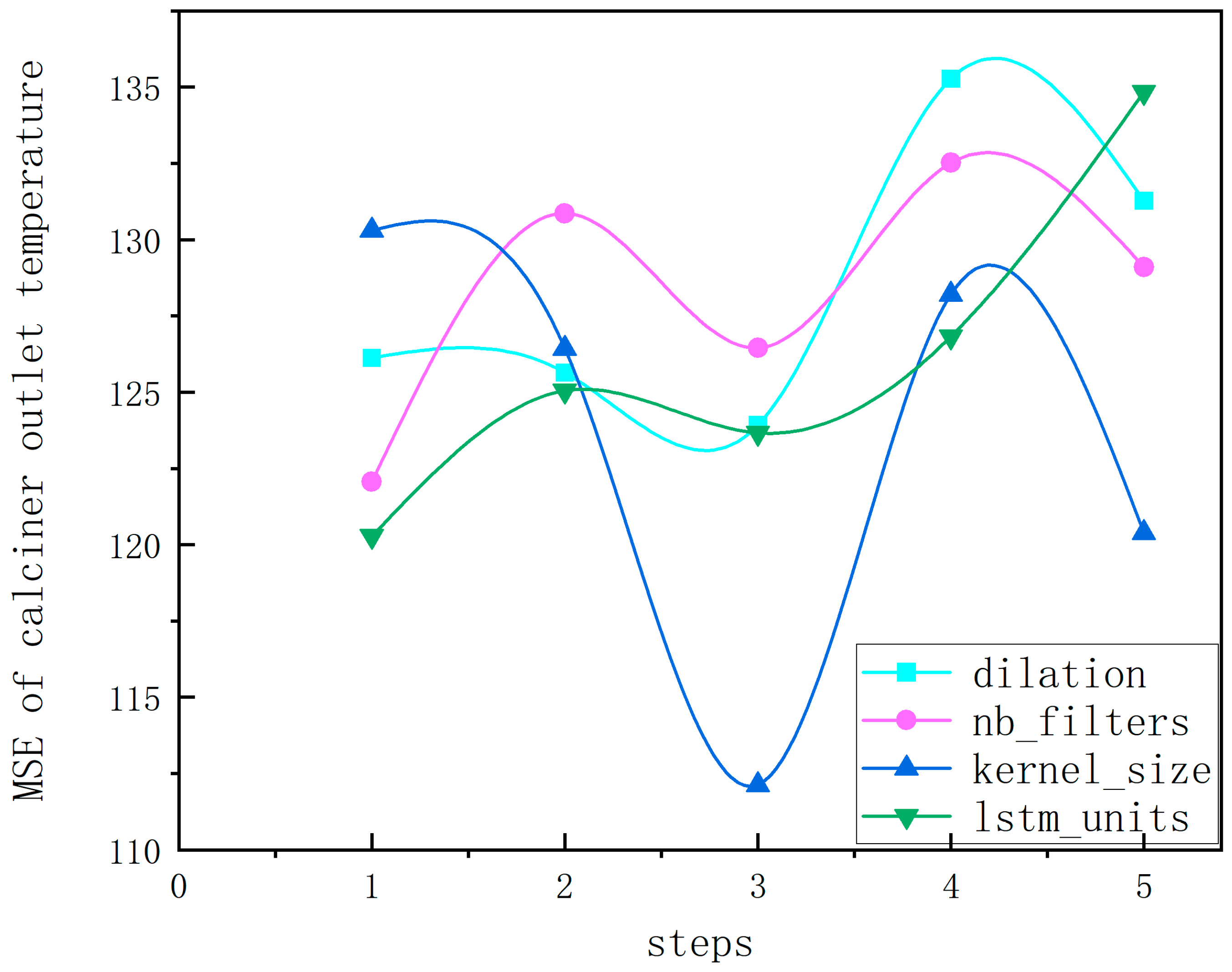
From Section 3, we know the TCN-BiLSTM hybrid model combines TCN and BiLSTM, and that parameters such as kernel size, dilation rate, filter size, and number of units critically influence performance. Table 3 presents various parameter combinations, offering rich options for model tuning. By adjusting these parameters, model performance under different configurations can be explored to identify optimal settings. As shown in Figure 9, varying a single parameter reveals its influence on MSE. The lowest error—and hence best model performance—is achieved when the kernel size is set to 8, dilation rate to [1, 2, 4, 8, 16], filter size to 18, and number of LSTM units to 64. To systematically evaluate the effectiveness of model architectures, this study employs a controlled variable approach for fair comparison. All models involved in the comparison, including the proposed TCN-BiLSTM and selected baseline models, are trained and tested under identical hyperparameter configurations.
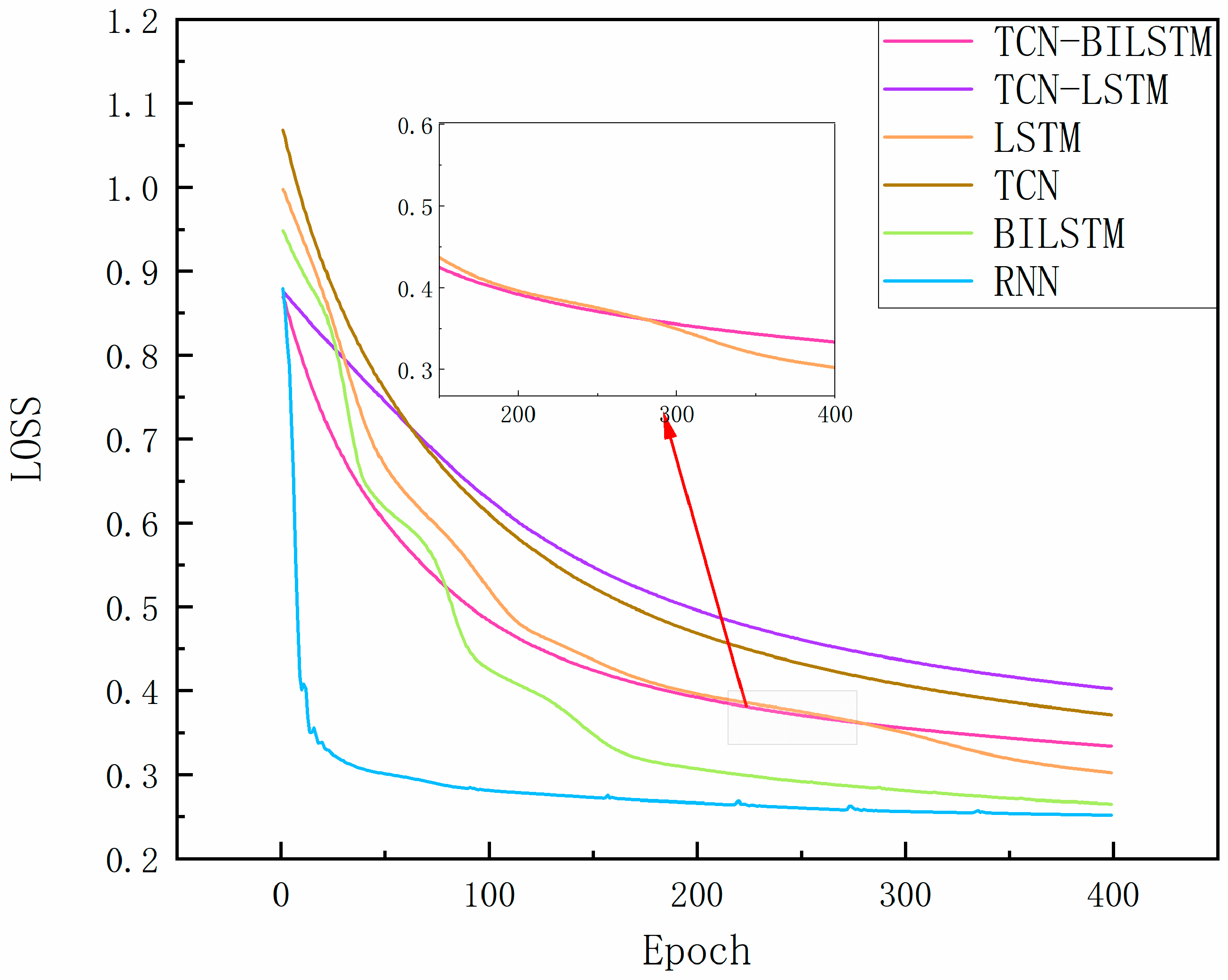
To validate the stability of the training process, Figure 10 presents the training loss convergence curves for each model. The losses of all models exhibit a smooth decline and eventual stabilization, indicating adequate and effective training. Notably, the TCN-BiLSTM model proposed in this study (represented by the black solid line) achieves the fastest convergence speed and the lowest stabilized loss value, providing intuitive evidence of its architectural effectiveness. This serves as procedural justification for the superior performance demonstrated in subsequent testing.

4.3. Prevention of Temporal Data Leakage

To ensure the causality of predictions, this study prevents future information leakage at both the model architecture and data preprocessing levels. At the model level, a causally constrained BiLSTM layer is employed, which applies masking to the backward LSTM to restrict its access to current and historical information only. At the data level, a strategy of sequential partitioning followed by separate normalization is adopted: standardization parameters are calculated exclusively from the training set and then applied separately to both the training and test sets, thereby eliminating information leakage during the preprocessing stage.

4.4. Comparative Analysis of Predictions

4.4.1. Short-Term Forecasting Analysis

This section presents a comparative analysis of the TCN-BiLSTM model against five other models in predicting one hour ahead, aimed at verifying the predictive performance of the TCN-BiLSTM model for the precalciner outlet temperature. As shown in Table 4, the comparison is based on the values of MSE, RMSE, MRE, and MAE. It can be seen that the RNN model has relatively high MSE (149.0311) and MAE (9.3357), indicating the limitations of traditional recurrent neural networks in modeling long sequences and their susceptibility to the vanishing gradient problem. The BiLSTM (MSE = 144.0579), TCN-LSTM (MSE = 127.1515), and LSTM (MSE = 120.0579) models perform at an intermediate level with generally moderate predictive accuracy. The TCN model (MSE = 116.3618), with its multi-scale feature extraction capability enabled by dilated convolution, ranks second in performance. The TCN-BiLST Mmodel, which integrates TCN’s local feature capturing with BiLSTM’s bidirectional temporal modeling, achieves the best prediction performance in industrial temperature forecasting scenarios that involve both local fluctuations and long-term patterns. Its MSE (112.1317), RMSE (10.5892), MRE (0.0091), and MAE (8.1598) are all lower than those of the other models. Specifically, its MSE is 3.6% lower, RMSE 1.8% lower, MRE 1.1% lower, and MAE 0.9% lower than the next-best TCN model. This also verifies the synergistic effect of the hybrid architecture.
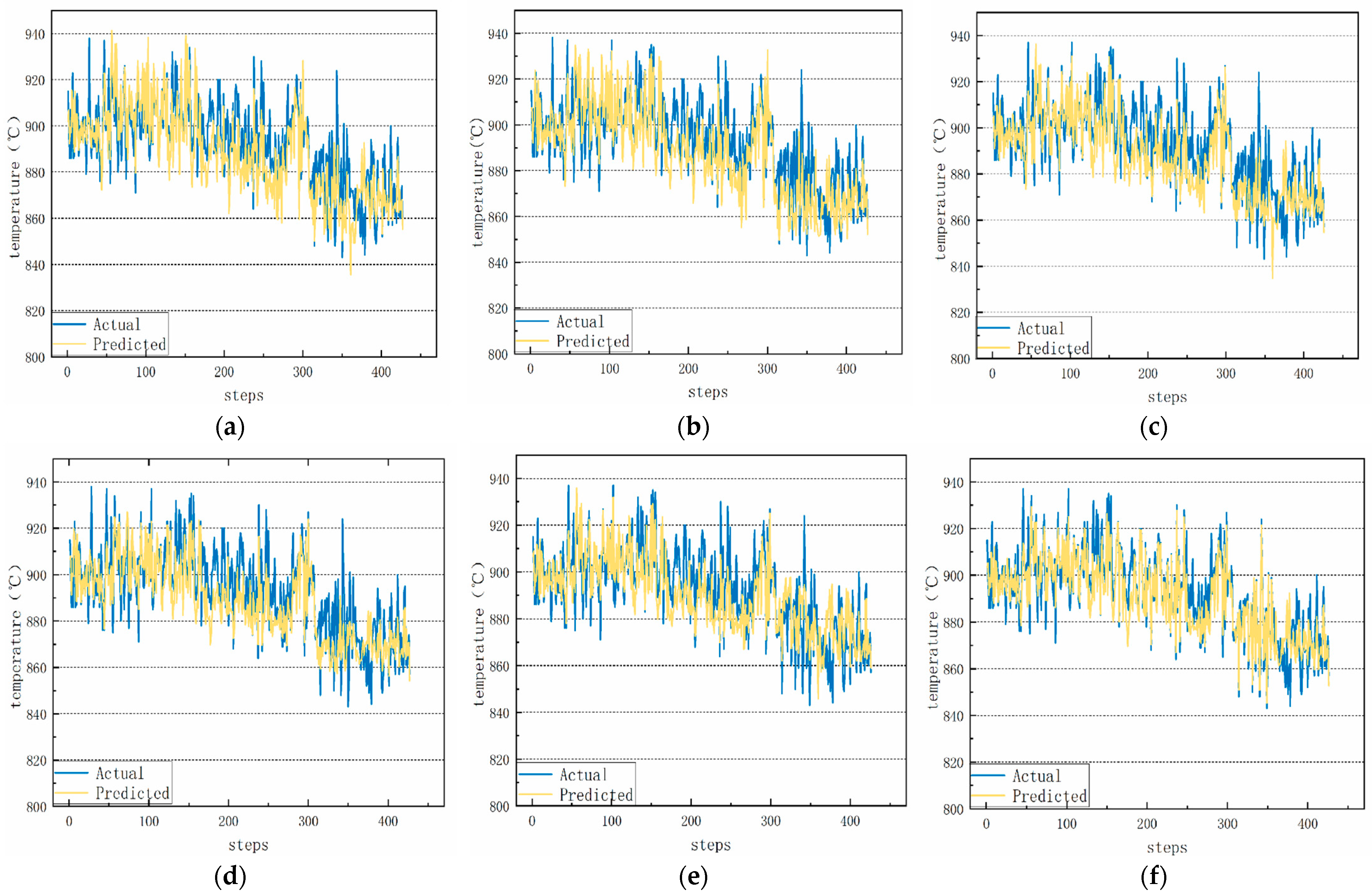
As shown in Figure 11, six models’ prediction curves for the next one hour are presented. The RNN model produces a smooth but noticeably lagging prediction curve, and its response to abrupt temperature changes is delayed. The BiLSTM model, due to its bidirectional structure, slightly improves trend tracking, but still fails to adequately capture sudden changes. The TCN-LSTM model significantly reduces peak prediction errors compared to RNN and BiLSTM, though it still shows minor overfitting fluctuations. The LSTM model’s gating mechanism effectively mitigates gradient issues, but it still exhibits lag during rapid transitions. The TCN model responds relatively well to abrupt changes but lacks in modeling long-range dependencies. The TCN-BiLSTM model shows relatively low peak error in the abrupt change segment, 15% lower than that of the TCN model, and has the least delay among all models. It also improves phase shift issues in long-term cycles.

4.4.2. Medium-Term Forecasting Analysis

A comparison is made between the TCN-BiLSTM model and the other five models in predicting the precalciner outlet temperature over the next twelve hours, to verify the prediction performance of the TCN-BiLSTM model. As shown in Table 5, the comparison is based on the values of MSE, RMSE, MRE, and MAE. It can be concluded that the error of the TCN-BiLSTM model is significantly lower than that of the other five models. Figure 12 illustrates the prediction performance of the six models for the precalciner outlet temperature over the next 12 h. Overall, the TCN-BiLSTM model demonstrates more accurate prediction results, with its prediction curve showing significantly higher coincidence with the real values than the other five models. This verifies its dual advantages in capturing short-term abrupt changes and modeling long-term dependencies in complex time-series data.

4.4.3. Long-Term Forecasting Analysis

A comparison is conducted between the TCN-BiLSTM model and the other five models in predicting the precalciner outlet temperature over the next twenty-four hours, to assess the prediction capability of the TCN-BiLSTM model. As shown in Table 6, the evaluation is based on the values of MSE, RMSE, MRE, and MAE. It can be concluded that the error of the TCN-BiLSTM model is significantly lower than that of the other five models. As shown in Figure 13, the TCN-BiLSTM model outperforms other models. Its prediction curve generally aligns well with the actual values, demonstrating stronger stability and robustness.
In summary, to validate the model’s forecasting ability under dynamic working conditions, predictions were tested for 1 h, 12 h, and 24 h into the future. TCN-BiLSTM showed the highest fitting accuracy in short-term forecasting (1 h), while in medium- and long-term forecasting (12 h and 24 h), although the error increased slightly, it still significantly outperformed the other five models. The TCN-BiLSTM model, by integrating temporal convolution and bidirectional long short-term memory networks, achieves a balance between error minimization and optimal dynamic response, outperforming single-structure models. It provides a reliable solution for modeling complex industrial time-series data and highlights the crucial role of hybrid architectures in the collaborative modeling of feature extraction and temporal dependency.

5. Discussion

This study demonstrates the superior performance of the TCN-BiLSTM model, which stems from the synergistic integration of TCN and causal BiLSTM. The TCN captures long-term temperature trends through dilated convolutions, while the causal BiLSTM enhances contextual modeling under strict temporal causality, together improving robustness in complex industrial dynamics. These results align with international advances in hybrid forecasting models, with our causal constraints refining the approach for industrial applications. Practically, the model enables high-precision feedforward control for decomposition furnaces, supporting operational adjustments and energy efficiency in process industries.
(1)
This study innovatively proposes a causally constrained TCN-BiLSTM hybrid architecture, which achieves synergistic enhancement through TCN’s long-term trend capture and BiLSTM’s bidirectional contextual modeling. The Spearman correlation coefficient is employed for key variable selection, ensuring predictive causality while providing a new reliable method for industrial time series forecasting.
(2)
The model enables high-precision, minutes-ahead temperature prediction for decomposition furnace operations, which can be directly applied to optimize real-time fuel and air distribution. This stabilizes thermal conditions, improves clinker quality, reduces energy consumption, and offers a feasible technical solution for intelligent control in cement production.
(3)
The current model’s performance relies on high-quality historical data, and its robustness to sensor anomalies or major process changes requires further validation. As a purely data-driven model, its integration with process mechanisms is insufficient, and its lightweight deployment in practical DCS systems necessitates additional research.
(4)
Future efforts will focus on developing self-learning models capable of adapting to operational condition changes, exploring deeper integration of data-driven and mechanistic models, and promoting the lightweight deployment and long-term operational validation of the model in edge computing environments.

Author Contributions

Conceptualization: M.D. and H.K. Methodology: M.D. and H.K. Software: M.D. Validation: M.D. Formal Analysis: M.D. and H.K. Investigation: M.D. Resources: M.D. and H.K. Data Curation: M.D. and H.K. Writing–Original Draft: M.D. Writing–Review & Editing: M.D. and H.K. Visualization: M.D. Supervision: H.K. Project Administration: H.K. Funding Acquisition: Not applicable. All authors have read and agreed to the published version of the manuscript.

Funding

This research received no external funding.

Data Availability Statement

The original contributions presented in this study are included in the article. Further inquiries can be directed to the corresponding author.

Acknowledgments

First and foremost, I express sincere gratitude to Kao Hongtao, my supervisor, for his invaluable guidance throughout this research. From defining the direction and conceiving the TCN-BiLSTM model to optimizing the experimental scheme and refining the manuscript, his rigorous academic attitude, profound scholarly accomplishments, and forward-looking vision greatly benefited me and laid a solid foundation for this work. I also thank the collaborating cement plant for providing real production data, which offered a reliable basis for model validation. Additionally, my thanks go to fellow laboratory colleagues and friends for their technical discussions and assistance, as well as my family for their unwavering silent support and understanding behind the scenes. All authors have read and agreed to the published version of the manuscript.

Conflicts of Interest

The authors declare no conflicts of interest.

References

  1. Zhou, H.; Zhang, Y.; Li, X.; Wang, C.; Liu, Y.; Chen, L.; Yang, M.; Xu, K.; Sun, L.; Wu, Q.; et al. Modeling and control of the clinker calcination process in rotary kilns: A review. Chem. Eng. Sci. 2020, 225, 115752. [Google Scholar]
  2. Kurdowski, W.; Duszak, S. Influence of precalciner temperature on free lime content and clinker phase composition in cement production. Cem. Concr. Res. 2018, 103, 123–134. [Google Scholar]
  3. Zhang, H.; Li, Y.; Wang, J.; Liu, B.; Chen, X.; Zhao, Y.; Sun, T.; Xu, L.; Zhou, W. Over-burning effect in cement clinker: Microstructure and grindability analysis. Constr. Build. Mater. 2019, 218, 497–506. [Google Scholar]
  4. Bai, S.; Kolter, J.Z.; Koltun, V. An empirical evaluation of generic convolutional and recurrent networks for sequence modeling. arXiv 2018, arXiv:1803.01271. [Google Scholar] [CrossRef]
  5. Schuster, M.; Paliwal, K.K. Bidirectional recurrent neural networks. IEEE Trans. Signal Process. 1997, 45, 2673–2681. [Google Scholar] [CrossRef]
  6. Vaswani, A.; Shazeer, N.; Parmar, N.; Uszkoreit, J.; Jones, L.; Gomez, A.N.; Kaiser, Ł.; Polosukhin, I. Attention is all you need. In Proceedings of the Advances in Neural Information Processing Systems, Long Beach, CA, USA, 4–9 December 2017; pp. 5998–6008. [Google Scholar]
  7. Rahman, M.A.; Zhang, T.; Lu, Y. PINN-CHK: Physics-informed neural network for high-fidelity prediction of early-age cement hydration kinetics. Neural Comput. Appl. 2024, 36, 13665–13687. [Google Scholar]
  8. Sun, C.; Liu, P.; Guo, H.; Di, Y.; Xu, Q.; Hao, X. Control of Precalciner Temperature in the Cement Industry: A Novel Method of Hammerstein Model Predictive Control with ISSA. Processes 2023, 11, 214. [Google Scholar] [CrossRef]
  9. Raza, A.; Mehmood, A.; Kim, H. Multivariate CNN with attention mechanism for rotary kiln temperature prediction. Appl. Therm. Eng. 2021, 189, 116682. [Google Scholar]
  10. Liu, G.; Wang, K.; Hao, X.; Zhang, Z.; Zhao, Y.; Xu, Q. SA-LSTMs: A new advance prediction method of energy consumption in cement raw materials grinding system. Energy 2022, 241, 122768. [Google Scholar] [CrossRef]
  11. Okoji, A.I.; Anozie, A.N.; Omoleye, J.A.; Taiwo, A.E.; Babatunde, D.E. Evaluation of adaptive neuro-fuzzy inference system-genetic algorithm in the prediction and optimization of NOx emission in cement precalcining kiln. Environ. Sci. Pollut. Res. Int. 2023, 30, 54835–54845. [Google Scholar] [CrossRef] [PubMed]
  12. Li, J.; Meng, P.; Liang, Y.; Li, J.; Miao, S.; Pan, Y. Research on lime rotary kiln temperature prediction by multi-model fusion neural network based on dynamic time delay analysis. Therm. Sci. 2024, 28, 2703–2715. [Google Scholar] [CrossRef]
  13. Yang, X.; Wang, Z.; Zhang, L.; Liu, Y.; Chen, H.; Li, M. Nonlinear modeling of cement rotary kiln based on BP neural network with adaptive learning rate. IEEE Trans. Ind. Inf. 2019, 15, 3254–3262. [Google Scholar]
  14. Wang, Y.; Li, Z.; Zhang, Q.; Liu, S.; Chen, W.; Zhou, T.; Xu, F.; Sun, H. Hybrid RNN-attention model for delayed process variables prediction in cement kilns. Control Eng. Pract. 2021, 112, 104812. [Google Scholar]
  15. Ali, A.; Kamal, K.; Ratlamwala, T.A.H.; Sheikh, M.F.; Arsalan, M. Power prediction of waste heat recovery system for a cement plant using back propagation neural network and its thermodynamic modeling. Int. J. Energy Res. 2021, 45, 9162–9178. [Google Scholar] [CrossRef]
  16. Santos, J.; Oliveira, R.; Costa, L. Deep reinforcement learning for rotary kiln temperature control in cement production. Ind. Eng. Chem. Res. 2020, 59, 6782–6790. [Google Scholar]
  17. Bontempi, G.; Ben Taieb, S.; Le Borgne, Y.A. Machine learning strategies for time series forecasting. In European Business Intelligence Summer School; Springer: Berlin/Heidelberg, Germany, 2013; pp. 62–77. [Google Scholar]
  18. Atmaca, A.; Yumrutaş, R. Thermodynamic and exergoeconomic analysis of a cement plant. Energy 2014, 64, 454–468. [Google Scholar]
  19. Liu, S.; Shen, W.; Wu, C.Q.; Lyu, X. Optimizing Temperature Setting for Decomposition Furnace Based on Attention Mechanism and Neural Networks. Sensors 2023, 23, 9754. [Google Scholar] [CrossRef] [PubMed]
  20. Zhang, K.; Liu, M.; Wang, X.; Chen, D.; Zhao, R.; Sun, P.; Li, J. Digital twin-driven temperature prediction for cement kilns using TCN-BiLSTM with attention mechanism. Appl. Energy 2023, 331, 120389. [Google Scholar]
  21. Duan, K.; Cao, S.; Li, J.; Xu, C. Prediction of neutralization depth of R.C. bridges using machine learning methods. Crystals 2021, 11, 210. [Google Scholar] [CrossRef]
  22. Schober, P.; Boer, C.; Schwarte, L.A. Correlation coefficients: Appropriate use and interpretation. Anesth. Analg. 2018, 126, 1763–1768. [Google Scholar] [CrossRef] [PubMed]
  23. Veit, A.; Wilber, M.; Belongie, S. Residual networks behave like ensembles of relatively shallow networks. In Proceedings of the Annual Conference on Neural Information Processing Systems, Montreal, QC, Canada, 5–10 December 2020; pp. 550–558. [Google Scholar]
  24. Srivastava, N.; Hinton, G.; Krizhevsky, A.; Sutskever, I.; Salakhutdinov, R. Dropout: A simple way to prevent neural networks from overfitting. J. Mach. Learn. Res. 2014, 12, 1929–1958. [Google Scholar]
  25. Zhou, X.; Wang, J.; Cao, X.; Fan, Y.; Duan, Q. Simulation of future dissolved oxygen distribution in pond culture based on sliding-window temporal convolutional network and trend surface analysis. Aquacult. Eng. 2021, 95, 102200. [Google Scholar] [CrossRef]
  26. Fan, J.; Zhang, K.; Huang, Y.; Zhu, Y.; Chen, B. Parallel spatio-temporal attention-based TCN for multivariate time series prediction. Neural Comput. Appl. 2023, 35, 13109–13118. [Google Scholar] [CrossRef]
  27. Yu, Y.; Si, X.; Hu, C.; Zhang, J. A review of recurrent neural networks: LSTM cells and network architectures. Neural Comput. 2019, 31, 1235–1270. [Google Scholar] [CrossRef]
  28. Wang, Y.; Xu, Y.; Shi, Y. Bi-directional LSTM with hierarchical attention for text classification. Expert Syst. Appl. 2022, 187, 115905. [Google Scholar]
  29. Hochreiter, S.; Schmidhuber, J. Long short-term memory. Neural Comput. 1997, 9, 1735–1780. [Google Scholar] [CrossRef] [PubMed]
  30. Lin, Q.; Yang, Z.; Huang, J.; Deng, J.; Chen, L.; Zhang, Y. A Landslide Displacement Prediction Model Based on the ICEEMDAN Method and the TCN-BiLSTM Combined Neural Network. Water 2023, 15, 4247. [Google Scholar] [CrossRef]
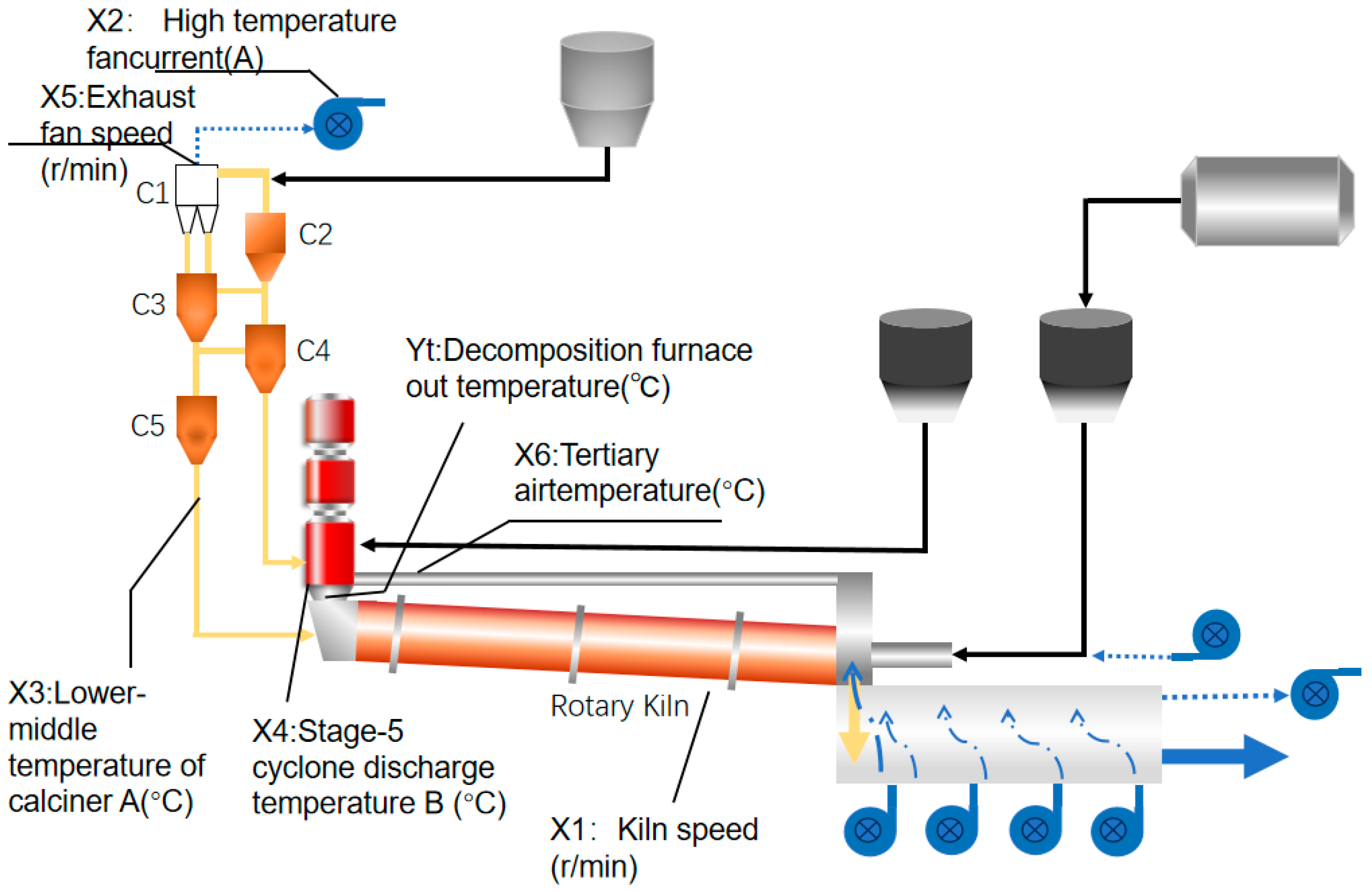
Figure 1. Production Process Flowchart of the Precalciner Kiln. (Arrows in different colors represent distinct paths: blue for air path and orange for material path).
Processes 13 04068 g001
Figure 2. Spearman correlation analysis.
Processes 13 04068 g002
Figure 3. Sensitivity Analysis of Key Operational Parameters on Outlet Temperature of the Precalciner.
Processes 13 04068 g003
Figure 4. Architecture of the residual block.
Processes 13 04068 g004
Figure 5. Structure of the causal dilated convolution.
Processes 13 04068 g005
Figure 6. Architecture of the BiLSTM neural network.
Processes 13 04068 g006
Figure 7. Structure of the TCN-BiLSTM hybrid model.
Processes 13 04068 g007
Figure 8. Error distribution across different algorithms.
Processes 13 04068 g008
Figure 9. Mean squared error (MSE) under different conditions.
Processes 13 04068 g009
Figure 10. Comparison of Training Loss Convergence Curves Among Different Models.
Processes 13 04068 g010
Figure 11. Comparison of 1-h ahead prediction results among different models. (a) RNN Prediction Results; (b) BILSTM Prediction Results; (c) TCN-LSTM Prediction Results; (d) LSTM Prediction Results; (e) TCN Prediction Results; (f) TCN-BiLSTM Prediction Results.
Processes 13 04068 g011aProcesses 13 04068 g011b
Figure 12. Comparison of 12-h ahead prediction results among different models. (a) RNN Prediction Results; (b) BILSTM Prediction Results; (c) TCN-LSTM Prediction Results; (d) LSTM Prediction Results; (e) TCN Prediction Results; (f) TCN-BiLSTM Prediction Results.
Processes 13 04068 g012
Figure 13. Comparison of 24-h ahead prediction results among different models. (a) RNN Prediction Results; (b) BILSTM Prediction Results; (c) TCN-LSTM Prediction Results; (d) LSTM Prediction Results; (e) TCN Prediction Results; (f) TCN-BiLSTM Prediction Results.
Processes 13 04068 g013
Table 1. Description of input and output variables for the TCN-BiLSTM prediction model.
Variable LabelPhysical MeaningSymbolUnit
X1Kiln speedKSrpm
X2High-temperature fan speedHTFSrpm
X3Mid-lower temperature of precalciner (A)Tpml°C
X4Stage-5 cyclone discharge temperature BT5t°C
X5Exhaust fan speedEFSrpm
X6Tertiary air temperatureTta°C
YtOutlet temperature of precalcinerTout°C
Table 2. Descriptive statistics of the key variables (N = 2128).
Input VariablesMaximumMinimumAverageStandard Deviation
Kiln rotation speed: X1 (r/min)4.732.414.0692636020.309318701
High-temperature fan speed: X2 (r/min)915654872.751407125.32727357
Lower-middle temperature of calciner A: X3 (°C)951739879.174953127.37702543
Outlet temperature of 5-stage cyclone B: X4 (°C)914685868.626641714.20531897
Exhaust gas fan speed: X5 (r/min)627472524.252345231.48491656
Tertiary air temperature of calciner: X6 (°C)1200873989.520637943.72847244
decomposer exit outlet temperature: Yt (°C)938837887.166979416.66492248
Table 3. Parameter configurations of the TCN-BiLSTM model.
Parameters\Code12345
kernel size678910
dilation[1, 2, 4][1, 2, 4, 8][1, 2, 4, 8, 16][1, 2,…, 32][1, 2,…, 64]
filter size1836547290
Lstm_units641282565121024
Table 4. Error metrics for 1-h ahead predictions.
ModelParameterMSERMSEMREMAE
RNNhidden size = 8145.671512.06950.01059.3536
BILSTMhidden size = 8141.570911.89840.01059.3994
TCN-LSTMhidden size = 8127.151511.27620.00988.7467
LSTMhidden size = 8120.057910.97770.00968.6183
TCNdilation = [1, 2, 4, 8, 16], kernel size = 8116.361810.78710.00928.2340
TCN-BiLSTMdilation = [1, 2, 4, 8, 16], kernel size = 8112.131710.58920.00918.1598
Table 5. Prediction error metrics for 12-h ahead forecasts.
ModelParameterMSERMSEMREMAE
RNNhidden size = 8146.566012.10650.01089.6102
BILSTMhidden size = 8143.956611.99820.01079.5764
TCN-LSTMhidden size = 8130.329911.41620.00998.8382
LSTMhidden size = 8129.023611.35890.00998.9034
TCNdilation = [1, 2, 4, 8, 16], kernel size = 8128.616511.34090.00988.7304
TCN-BiLSTMdilation = [1, 2, 4, 8, 16], kernel size = 8115.885810.76500.00948.4366
Table 6. 24-h ahead prediction error metrics.
ModelParameterMSERMSEMREMAE
RNNhidden size = 8150.301412.25990.01059.3184
BILSTMhidden size = 8144.057912.00240.01049.3361
TCN-LSTMhidden size = 8138.550911.77080.01029.2987
LSTMhidden size = 8137.949611.74520.01029.2074
TCNdilation = [1, 2, 4, 8, 16], kernel size = 8134.902911.61480.00978.6997
TCN-BiLSTMdilation = [1, 2, 4, 8, 16], kernel size = 8118.579610.88940.00958.5002
Disclaimer/Publisher’s Note: The statements, opinions and data contained in all publications are solely those of the individual author(s) and contributor(s) and not of MDPI and/or the editor(s). MDPI and/or the editor(s) disclaim responsibility for any injury to people or property resulting from any ideas, methods, instructions or products referred to in the content.