Beyond Static Fingerprints to Dynamic Evolution: A CNN–LSTM–Attention Model for Identifying Coal Mine Water Inrush Sources in Northern China

Abstract

Mine water inrush poses a severe threat to coal mine safety, making rapid and accurate identification of water sources essential. Existing methods, including conventional hydrochemical diagrams and machine learning, struggle with high-dimensional, nonlinear hydrogeochemical data characterized by implicit temporal dynamics. This study proposes an intelligent identification model integrating convolutional neural networks (CNNs), long short-term memory (LSTM), and an attention mechanism (CNN–LSTM–Attention). The model employs a CNN to extract local fingerprint features from hydrochemical indicators (K⁺+Na⁺, Ca²⁺, Mg²⁺, Cl⁻, SO₄²⁻, and HCO₃⁻), uses LSTM to model evolutionary patterns, and leverages an attention mechanism to adaptively focus on critical discriminative features. Based on 76 water samples from the Tangjiahui Coal Mine, the model achieved 91% accuracy on the test set, outperforming standalone CNN, LSTM, and CNN–LSTM models. Visualization of attention weights further revealed key diagnostic indicators, enhancing interpretability and bridging data-driven methods with hydrogeochemical mechanisms. This study provides a powerful and interpretable tool for water inrush source identification, supporting the transition toward intelligent and transparent coal mine water hazard prevention.

1. Introduction

Safe and efficient coal production is a cornerstone of national energy security, yet it remains persistently threatened by geological hazards [1,2]. Among these, mine water inrush, characterized by sudden onset, destructive force, and rescue difficulties, has long posed a major challenge to the sustainable development of the coal industry [3,4]. In China, water-related accidents rank second in fatalities among major coal mine disasters, causing severe economic losses and social consequences [5,6]. Fundamentally, water inrush occurs when large volumes of groundwater, driven by high hydraulic pressure, rapidly enter underground workings through conductive pathways such as faults, fracture zones, or collapse columns [7,8,9]. Consequently, rapid and accurate identification of water sources is crucial, not only for post-disaster emergency responses, such as determining sealing targets or devising drainage strategies, but also for hydrogeological assessment, hazard forecasting, and the formulation of preventive measures [10,11,12].

Traditionally, source identification has relied heavily on hydrogeologists’ expert judgment, based on aquifer burial conditions, hydraulic monitoring, and limited hydrochemical data [13,14]. This reliance introduces subjectivity and delay, and misclassification can result in missed rescue opportunities and ineffective mitigation, with potentially catastrophic outcomes [15,16]. Therefore, the development of objective, precise, efficient, and intelligent identification methods is urgently needed to transition from “experience-driven” to “data-driven” paradigms [17,18]. Achieving this transformation is of great theoretical and practical significance for modernizing water hazard prevention in coal mines, safeguarding miners’ lives, and preventing property loss [19,20]. The central aim of this study is to extract nonlinear relationships between complex hydrogeochemical features and water source categories in order to construct a high-performance intelligent identification model to support coal mine safety.

Over decades of research, methods for source identification have evolved from traditional to modern approaches, each with distinct strengths and limitations [21,22]. Early studies primarily relied on hydrogeological investigations, including borehole drilling to analyze aquifer lithology, thickness, burial depth, and water abundance, combined with hydraulic monitoring to assess inter-aquifer connectivity [23,24]. While fundamental for understanding hydrogeological conditions, these methods cannot provide precise “fingerprint” tracing of inrush sources [25,26]. Hydrochemical analysis subsequently became the dominant and “gold-standard” technique. Based on the principle that aquifers formed under different geological ages and depositional environments (e.g., Quaternary pore water, Carboniferous–Permian sandstone fissure water, Ordovician karst water) exhibit unique geochemical signatures due to variations in lithology, water–rock interactions, and flow conditions, researchers have applied ionic compositions (K⁺, Na⁺, Ca²⁺, Mg²⁺, Cl⁻, SO₄²⁻, HCO₃⁻), isotopes (δD, δ¹⁸O), and trace elements (e.g., Sr, Br) for source discrimination [27,28,29]. Tools such as Piper trilinear diagrams, Gibbs plots, ion ratio methods, and statistical approaches including cluster analysis (CA) and principal component analysis (PCA) have been widely used [30,31,32]. Although effective, these methods remain highly dependent on expert interpretation and are challenged by ambiguous hydrochemical signatures or strong mixing effects, which reduce classification accuracy.

With the rise of machine learning (ML), data-driven intelligent identification models have become more prominent [33,34,35,36]. Early applications employed traditional algorithms such as support vector machine (SVM), random forests (RF), and naive Bayes classifier, all of which can automatically learn classification rules from hydrochemical data, thereby reducing subjectivity and improving the handling of high-dimensional datasets [37,38]. However, these models are inherently “shallow” learners, relying heavily on complex feature engineering and prior knowledge; moreover, they struggle to capture deep nonlinear relationships and temporal dynamics. Hydrochemical data are not static snapshots but evolve dynamically under mining influences, carrying valuable hydrogeological information that conventional ML approaches cannot fully exploit [39]. Thus, the development of advanced models capable of automatically extracting deep features and capturing temporal dependencies from high-dimensional hydrochemical data has become an inevitable trend.

Despite these challenges, ML applications in source identification have demonstrated substantial potential and achieved notable successes. For example, SVM maintained strong performance even with small sample sizes via identification of the optimal hyperplanes that effectively separate aquifer types [40]. RF, leveraging ensemble learning, not only achieves high accuracy but also ranks feature importance, thereby revealing the key hydrochemical indicators (e.g., Na⁺+K⁺, HCO₃⁻) that most contribute to classification [41]. Such insights enhance interpretability and support hydrogeochemical analyses. These successes validate the applicability of data-driven approaches, yet they do not fully resolve the bottlenecks of feature extraction and temporal information utilization [42].

Recent advances in deep learning (DL) may provide solutions to these limitations [43,44]. CNNs possess strong capabilities for local feature extraction and hierarchical representation, treating hydrochemical samples as one-dimensional vectors analogous to image pixels and automatically learning complex nonlinear feature combinations without manual selection [45]. LSTM, as a variant of recurrent neural networks, is specifically designed for sequential data, employing gated mechanisms to capture the long-term dependencies and dynamic variation capabilities essential for understanding hydrochemical changes under mining conditions [46]. However, CNNs alone are limited in modeling long-term dependencies, while LSTM is less effective in hierarchical abstraction.

To address these gaps, this study proposes a hybrid CNN–LSTM–Attention model. The framework first applies CNNs to extract high-level features from raw hydrochemical data and then feeds these sequences into LSTMs to capture temporal dependencies and dynamic evolution [47]. Finally, the attention mechanism adaptively assigns weights to different time steps, enabling the model to focus selectively on decisive features while suppressing noise. This synergistic design—CNNs for deep feature extraction, LSTM for temporal modeling, and an attention mechanism for interpretability—facilitates comprehensive analysis of both static fingerprints and dynamic evolutions in hydrochemical data [48,49]. Ultimately, the proposed model achieves more accurate and interpretable source identification of mine water inrush, offering a robust innovation for advancing coal mine water hazard prevention toward intelligent and transparent practices. Unlike typical applications that use explicit time-series data (e.g., stock prices, sensor readings), we innovatively treat the static hydrochemical fingerprint of a single water sample as a 1D sequential input. This allows the LSTM to model the implicit geochemical evolution and relationships between ions (e.g., the co-evolution of Ca²⁺ and SO₄²⁻ in limestone aquifers), which is a novel conceptualization in this field. The primary goal of integrating the attention mechanism in our work extends beyond a mere performance boost. It is explicitly used as a tool for hydrogeochemical interpretation. We validate the attention weights by correlating them with SHAP analysis and known geochemical principles (e.g., high attention on SO₄²⁻ for Ordovician water). This focus on using the architecture to generate scientifically plausible explanations, rather than as a black-box predictor, is a significant departure from many existing applications. The model is specifically designed and validated for the high-stakes task of water inrush source identification in coal mines. This necessitates a framework that is not only accurate but also robust and interpretable for practical decision-making by mine engineers and hydrogeologists. The integration of the three components is fine-tuned for this specific objective, differing from more generic implementations. In summary, our contribution lies in the novel application, adaptation, and interpretation of this established architecture to solve a critical geoscientific problem, with a strong emphasis on transparency and physical consistency.

The key innovations of our work lie in the following aspects: (1) While hydrochemical data are often treated as static, we constructed pseudo-time-series inputs to capture the dynamic evolution patterns of aquifers, which traditional methods (e.g., Piper diagrams, SVM, RF) cannot adequately represent. (2) Beyond high accuracy, we emphasize model transparency. The attention mechanism allows us to visualize and interpret the contribution of key ions (e.g., SO₄²⁻, Ca²⁺) in classification, aligning data-driven decisions with domain knowledge. (3) This is the first systematic application of the CNN–LSTM–Attention fusion model to water inrush source identification in the Tangjiahui Coal Mine. We provide a complete technical pathway from data collection and model construction to interpretable output, ensuring practical deployability.

2. Materials and Methods

2.1. Sampling and Analytical Procedures

A total of 76 groundwater samples (Figure 1) were collected and analyzed for their hydrochemical compositions: 33 samples from the sandstone aquifer above the No. 6 coal seam (The No. 6 coal seam is the primary minable seam in the study area, typically overlain by sandstone aquifers (roof aquifer) and underlain by another sandstone aquifer (floor aquifer), with the Ordovician limestone aquifer situated further below in the stratigraphic sequence) roof (roof aquifer water, RW), 20 samples from the sandstone aquifer beneath the No. 6 coal seam floor (floor aquifer water, FW), and 23 samples from the Ordovician limestone aquifer (Ordovician aquifer water, OW). Samples were collected into pre-cleaned and sterilized 5 L high-density polyethylene bottles [50], which were rinsed two to three times with the corresponding source water prior to collection. Bottles were then sealed, labeled, and transported for analysis. All samples were obtained from surface or underground observation wells.

Six major hydrochemical parameters (Na⁺+K⁺, Ca²⁺, Mg²⁺, Cl⁻, SO₄²⁻, and HCO₃⁻) were determined for each sample. Onsite filtration through a 0.45 μm membrane was conducted prior to laboratory analysis at the Testing Center of Anhui University of Science and Technology [51]. Cation samples were stored in acid-cleaned 550 mL polypropylene bottles and acidified to pH < 2 with high-purity HNO₃ [52]. Anions (Cl⁻, SO₄²⁻, HCO₃⁻) were analyzed using Ion Chromatography (Dionex 120, Thermo Fisher Scientific, USA), while cations (Na⁺+K⁺, Ca²⁺, Mg²⁺) were determined using Inductively Coupled Plasma Atomic Emission Spectroscopy (ICP-AES, Thermo Fisher Scientific, USA) [53]. Due to the low concentration of K⁺, the contents of Na⁺ and K⁺ were combined as a single variable (Na⁺+K⁺) for analysis. All ion measurements were completed within 24 h of sampling. Ionic charge balance errors were calculated using the Aq•QA software 1.1 package [54], with all samples meeting the acceptable threshold of <5% [15].

Table 1. Water sample statistics.

Aquifers	Statistics	Concentration (mg/L)
		Ca2+	K+ + Na+	Mg2+	Cl−	SO42−	HCO3−
RW (n = 33, Type 2)	Min.	44.97	134.49	11.16	72.98	120.03	230.63
	Max.	103.23	416.77	36.59	566.08	210.66	463.07
	Mean	78.87	259.84	22.91	288.68	160.24	340.04
	Standard deviation	12.48	110.89	5.53	182.25	22.16	57.93
	C.V	0.16	0.43	0.24	0.63	0.14	0.17
FW (n = 20, Type 3)	Min.	128.78	180.47	29.15	307.69	203.31	232.44
	Max.	204.41	432.60	58.30	842.21	249.85	457.62
	Mean	160.15	277.79	47.72	454.34	224.87	396.15
	Standard deviation	17.28	72.34	7.09	148.67	13.06	56.50
	C.V	0.11	0.26	0.15	0.33	0.06	0.14
OW (n = 23, Type 1)	Min.	69.50	306.41	14.88	433.93	146.97	141.64
	Max.	122.64	633.41	37.21	962.53	240.05	348.66
	Mean	91.41	427.79	22.33	581.51	189.15	284.24
	Standard deviation	14.22	83.32	4.98	146.22	27.68	49.12
	C.V	0.16	0.19	0.22	0.25	0.15	0.17

presents the statistical summary for RW, FW, and OW. CO₃²⁻ accounted for less than 5% of the combined carbonate and bicarbonate content and was therefore excluded from compositional analyses. For cations, Na⁺+K⁺ exhibited the highest mean concentration across all aquifers, followed by Ca²⁺ and Mg²⁺. For anions, Cl⁻ was most abundant, followed by HCO₃⁻ and SO₄²⁻. In all aquifers, coefficients of variation were <1, indicating low variability and suggesting potential hydraulic connectivity.

2.2. CNN Architecture

CNNs are widely recognized for their capability to automatically extract local features and have achieved outstanding success in domains such as image recognition. In this study, each water sample, characterized by n hydrochemical parameters, was treated as a one-dimensional (1D) feature vector and fed into a 1D–CNN. Here, the CNN functions as a high-efficiency feature extractor, automatically learning deep, discriminative local patterns (e.g., ion combination ratios) from raw high-dimensional data, thus replacing the labor-intensive feature engineering (FE) typical of traditional machine learning.

The CNN module included the following [55]:

(1) Input Layer: Accepts input arrays of shape (None, n), where None refers to batch size and n to the number of input parameters.

(2) 1D Convolutional Layer: Multiple convolutional kernels slide across the input vector to detect local feature patterns:

$$h_i=f\left({\sum }_{j=1}^k{w}_j·x_{i+j-1}+b\right)$$

(1)

where w_j are kernel weights, b is bias, k is kernel size, x is the input vector, and f is the activation function.

(3) Activation Function: The Rectified Linear Unit (ReLU) was used to introduce non-linearity.

(4) Pooling Layer: A 1D Max Pooling layer reduced feature dimensionality, preserved salient patterns, and mitigated overfitting.

Stacked convolution and pooling stages generated a high-level abstract feature sequence subsequently processed by the LSTM module (Figure 2).

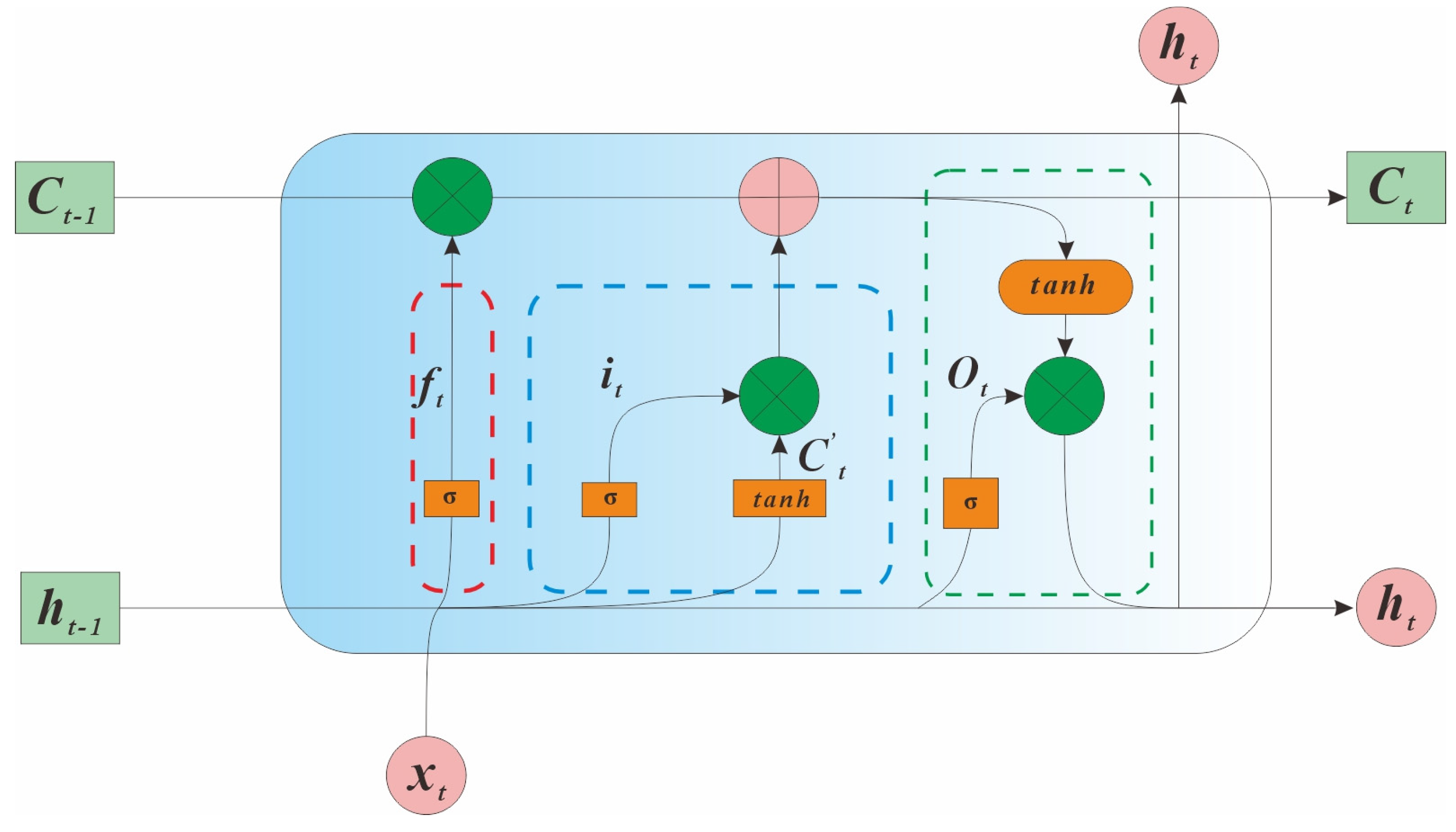
2.3. LSTM Network

Long short-term memory (LSTM) networks, a special type of recurrent neural network (RNN), address the vanishing/exploding gradient problem through gated mechanisms, enabling them to capture long-term dependencies.

In this study, the LSTM acted as a temporal modeling module. Although individual water samples are static, hydrogeochemical processes exhibit intrinsic sequential characteristics (e.g., long-term variation in ion concentrations). LSTM was used to model these dependencies from the CNN-extracted feature sequences.

An LSTM unit consists of three gates [56,57]:

(1) Forget Gate: Determines which information to discard.

$$f_t=\sigma \left(W_f·\left[h_{t-1},x_t\right]+b_f\right)$$

(2)

(2) Input Gate: Determines which new information to store.

$$i_t=\sigma \left(W_i·\left[h_{t-1},x_t\right]+b_i\right)$$

(3)

$${\tilde{C}}_t=tanh\left(W_C·\left[h_{t-1},x_t\right]+b_C\right)$$

(4)

(3) Output Gate: Determines the information to output.

$$o_t=\sigma \left(W_o·\left[h_{t-1},x_t\right]+b_o\right)$$

(5)

$$h_t=o_t\ast \mathrm{t}\mathrm{a}\mathrm{n}\mathrm{h}\left(C_t\right)$$

(6)

where σ is the sigmoid activation, tanh is the hyperbolic tangent, ∗ is element-wise multiplication, W and b are trainable weights and biases, x_t is the input at time t, and h_t−1 and C_t−1 are the hidden and cell states at time t − 1. The candidate cell state ${\tilde{C}}_t$ is generated by the hyperbolic tangent function (tanh). The forget gate (f_t), input gate (i_t), and output gate (o_t) regulate the flow of information through the sigmoid function (σ).

The CNN feature sequence was input to the LSTM layer, whose hidden states encoded the contextual information of the entire sequence (Figure 3).

2.4. Attention Mechanism (AM)

The attention mechanism (AM), inspired by the selective focus of human visual attention, enables a model to assign varying levels of importance to different parts of its input, effectively “focusing” on the most informative components [58,59]. Within our framework, AM functions as a critical information focuser, recognizing that not all hydrochemical parameters or temporal steps contribute equally to the final classification of water source types. For example, the SO₄²⁻ concentration may be particularly important for identifying Ordovician aquifer water (OW), whereas HCO₃⁻ may serve as a stronger indicator of floor aquifer water (FW).

The AM module automatically learns and computes an importance weight for each time step in the LSTM output sequence, thereby amplifying the influence of key discriminative features while suppressing irrelevant or noisy information. This selective emphasis enhances both the accuracy and interpretability of the model’s predictions.

The computation procedure is as follows [60,61]:

(1) Attention scores: For the hidden sequence H = (h₁, h₂, …, h_T), a small feedforward network computes scores α_t

$$u_t=\mathrm{t}\mathrm{a}\mathrm{n}\mathrm{h}\left(W_a{h}_t+b_a\right)$$

(7)

$${\alpha }_t={\displaystyle \frac{exp\left(u_t\right)}{{\sum }_{t=1}^{T}exp\left(u_t\right)}}$$

(8)

(2) Context vector: Weighted sum of hidden states

$$c={\sum }_{t=1}^T{\alpha }_t{h}_t$$

(9)

The context vector c represents the abstracted hydrochemical data, emphasizing the most discriminative features.

2.5. CNN–LSTM–Attention Model Construction

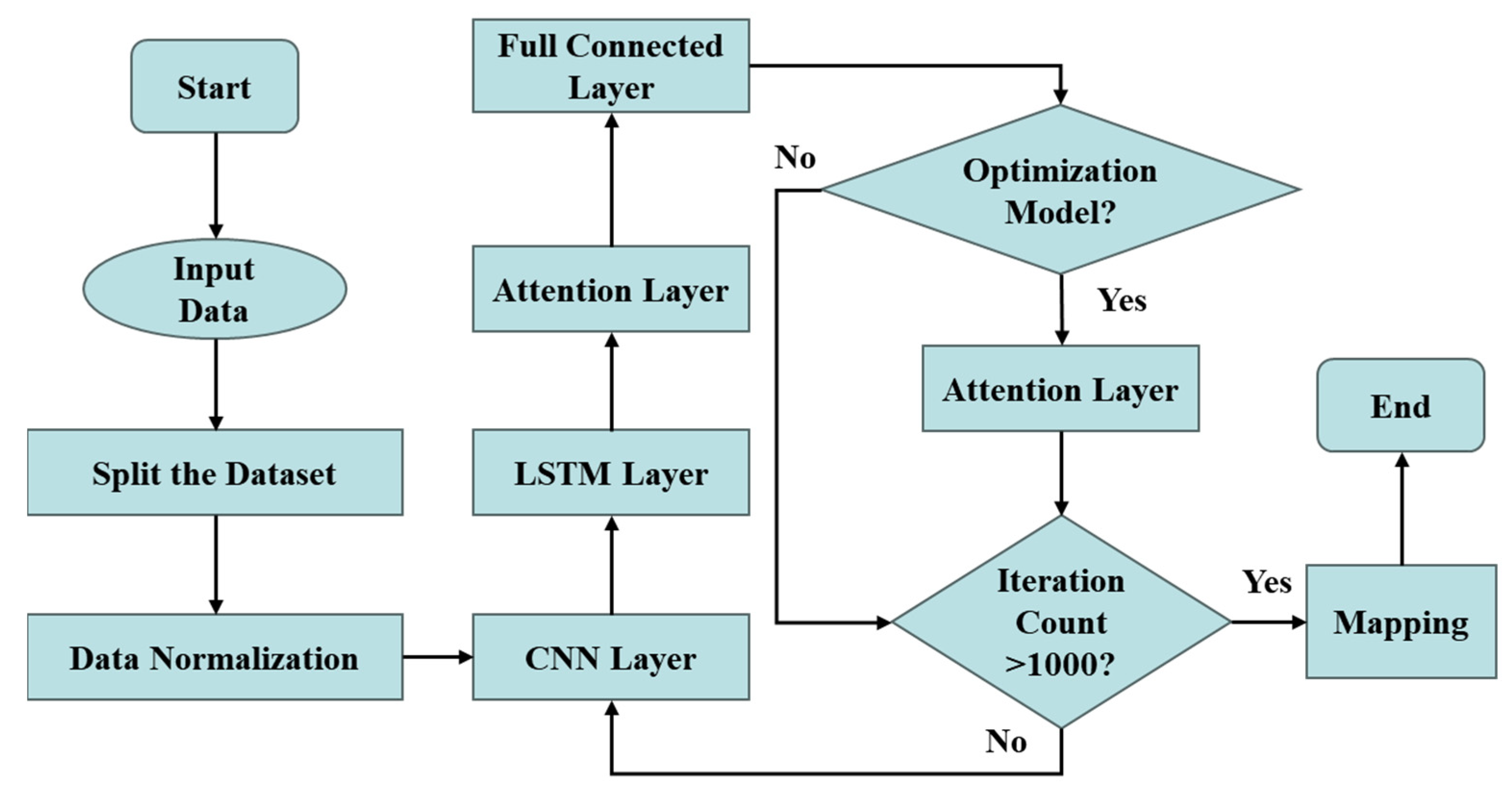
The three modules were combined into an end to end CNN–LSTM–Attention model (Figure 4).

(1) Input layer: Standardized hydrochemical time-series data.

(2) Feature extractor: 1–2 convolutional and pooling layers to extract local features.

(3) LSTM layer: Captures long-term dependencies from CNN outputs.

(4) Attention layer: Computes weighted context vector.

(5) Output layer: Fully connected layer with Softmax activation to generate class probabilities:

$$\widehat{y}=Softmax\left(W_{o}c+b_o\right)$$

(10)

Here, $\widehat{y}$ is the probability vector and W_o and b_o are the weights and biases of the output layer.

The flowchart of the CNN–LSTM–Attention model is shown in Figure 4, and the process encompasses the following steps (Figure 5):

Step 1: Input dataset with Na⁺+K⁺, Ca²⁺, Mg²⁺, Cl⁻, SO₄²⁻, and HCO₃⁻ as features.

Step 2: Divide the dataset into the training sample and test sample sets. During the dataset splitting phase, samples were shuffled randomly before being divided into training and testing sets. Given the limited total dataset size (n = 76), we employed a stratified random split to divide the data into a training set and an independent test set at a ratio of approximately 7:3. This resulted in 53 samples for training and 23 samples for testing. Stratification was used to ensure that the proportion of each water source type (RW, FW, OW) was preserved in both the training and test sets, preventing significant distributional shift.

Step 3: Normalize features to eliminate scale effects. We employed a multi-faceted strategy to ensure model generalization and robust performance evaluation:

(1) k-Fold Cross-Validation: To obtain a reliable estimate of model performance and mitigate the impact of a specific random split, we performed 5-fold cross-validation on the training set for model development and hyperparameter tuning. The results show a narrow distribution of accuracy across folds.

(2) Independent Test Set: The final model, selected based on cross-validation performance, was evaluated only once on the held-out test set (23 samples) to report the final performance metrics (91% accuracy). This set was not used during training or validation, providing an unbiased estimate of generalization to unseen data.

(3) Regularization Techniques: We incorporated built-in regularization methods to prevent overfitting. These included dropout layers within the LSTM and CNN components, the use of max-pooling, and the implementation of early stopping during training by monitoring the validation loss with a patience of 50 epochs.

This combined approach ensures that the model’s performance is not the result of overfitting to a particular data partition and that it generalizes effectively.

Step 4: Convolutional Neural Network (CNN) Layer. The normalized groundwater dataset is fed into the convolutional layer, where a set of trainable filters slide across the time-series data. Each filter extracts a specific type of feature, generating feature maps that capture the groundwater characteristics derived from the raw input data.

Step 5: Long Short-Term Memory (LSTM) Layer. The LSTM layer performs computations based on its hidden states. During training, the model automatically retains the version that achieves the best performance on the validation set, which is subsequently used for prediction tasks. We did not treat each sample as an independent vector. Instead, we used a sliding window approach or sample reordering to construct pseudo-time-series from samples of the same aquifer type, simulating the spatiotemporal evolution of hydrogeochemical processes. Specifically, the six ion indicators in each sample were treated as a sequence with time_steps = 6 and features = 1, enabling the LSTM to capture synergistic variations and evolutionary trends among ions.

Step 6: Attention Layer. Attention weights are computed for each output sequence, reflecting their relative importance in source classification. By multiplying these weights with the original input data, the model emphasizes the critical features that most strongly influence the classification of water sources.

Step 7: Fully Connected Layer. The extracted features are integrated and transformed into feature vectors suitable for output.

Step 8: The model verifies whether the predefined number of training iterations has been reached. If so, training terminates; otherwise, the process returns to Step 4 for continued optimization.

2.6. Model Evaluation

Model training employed categorical cross-entropy as the loss function and the Adam optimizer for parameter updates. In addition, we monitored validation loss with a patience of 50 epochs (for example), and training was halted if no improvement was observed. A maximum of 1000 epochs was set as a fallback, but training typically converged much earlier. Validation sets were used to monitor performance, and early stopping was applied to prevent overfitting. Final performance was evaluated on the independent test set, using accuracy, precision, recall, and F1 score, and compared with standalone CNN, LSTM, and CNN–LSTM models to demonstrate the superiority of the proposed framework.

3. Results and Discussion

3.1. Sensitivity Analysis of Model Parameters

a. Convolutional Layer. The number and size of convolution kernels exert a significant influence on model performance. (i) The number of kernels determines the quantity of feature maps. An excessive number may lead to redundant feature extraction, increased computational complexity, and a heightened risk of overfitting. Conversely, too few kernels may fail to capture sufficient features, resulting in underfitting. (ii) Kernel size affects the ability to capture local features. Larger kernels are inclined to capture global information but often neglect local details and increase computational costs. Smaller kernels better preserve local details but may overlook global patterns.

b. Pooling Layer. The pooling operation primarily performs downsampling to reduce the dimensionality of feature maps. When the pooling window size is set to 1, no pooling is performed, and the original feature map dimensions are preserved, thereby retaining more information but increasing computational burden. In contrast, pooling significantly reduces computational cost but may result in partial information loss.

c. LSTM Layer.

(i) Number of neurons. Determines the capacity for capturing temporal features. An excessively large number increases both overfitting risk and computational complexity, while too few neurons may fail to adequately capture temporal dependencies.

(ii) Time steps. Specifies the sequence length processed by the LSTM. Overly long time steps may cause gradient vanishing or explosion and increase computational costs, whereas short time steps may hinder the capture of long-term dependencies.

(iii) Learning rate. Controls the step size for optimizer weight updates. A high learning rate may cause instability or divergence during training, whereas a low rate slows convergence and increases the likelihood of local optima.

(iv) Batch size. Specifies the number of samples used in each weight update. Larger batch sizes increase memory consumption but enhance stability, while smaller batches may destabilize training but improve the chances of escaping local optima.

After iterative adjustment and verification, the final CNN–LSTM–Attention model parameters were determined (

Table 2. CNN–LSTM–Attention parameters.

Layer	Parameter	Value
Convolution	Number of filters Kernel size	64 5
Pooling	Pooling window size Pooling kernel size Stride	1 2 2
LSTM	Units Time steps Learning rate Batch size Epochs	64 36 0.001 32 1000

). The convolutional layer employs wide kernels to capture richer features and suppress noise interference. The pooling layer adopts max-pooling with zero-padding at the boundaries to retain essential information without altering output dimensions. The LSTM layer uses the Adam optimizer to minimize the cross-entropy loss function, thereby improving efficiency and reducing training time. Both the convolutional and LSTM layers use the ReLU activation function. The model was developed in Matlab R2021b using TensorFlow 2.5/Keras 2.5. The model configuration was as follows: the CNN module used 64 filters (size = 5, ReLU) with max-pooling (size = 2, stride = 2); the LSTM module had 64 units (tanh/sigmoid activations); and a single-layer attention network was used for feature scoring. Training was conducted with the Adam optimizer (lr = 0.001, β1 = 0.9, β2 = 0.999), a batch size of 32, and early stopping (patience = 50). Data preprocessing, analysis, and visualization were performed with Scikit-learn 1.8, NumPy 2.0, Pandas 2.3.0, Matplotlib 3.10.3/Seaborn 0.13.2, and SHAP 0.42.1. Furthermore, automated hyperparameter optimization frameworks (e.g., Optuna, Ray Tune) will be explored to more systematically and efficiently identify the optimal model configuration.

3.2. Analysis of Model Prediction Performance

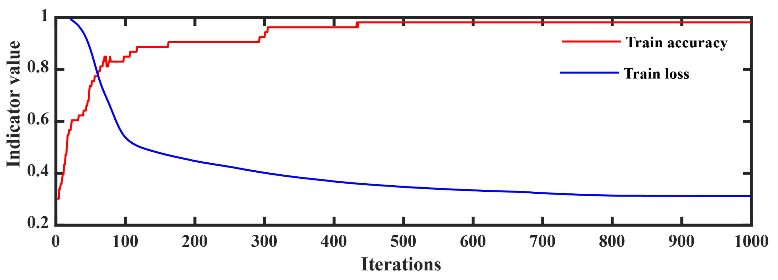
The training performance of the CNN–LSTM–Attention model (Figure 6) demonstrates a stable optimization trend. The training loss consistently decreases, indicating that the model effectively learns from the training data while progressively reducing prediction error. Meanwhile, the validation loss also declines, albeit with minor fluctuations, confirming continuous improvement in validation performance.

As training progresses, training accuracy steadily improves and eventually stabilizes, reflecting strong fitting capability and learning efficiency. Validation accuracy exhibits a similar upward trend, gradually stabilizing at a high level, suggesting robust generalization. Collectively, these results indicate that the model exhibits excellent learning behavior, convergence, and generalization, enabling accurate adaptation to unseen data. This lays a solid foundation for practical engineering applications. 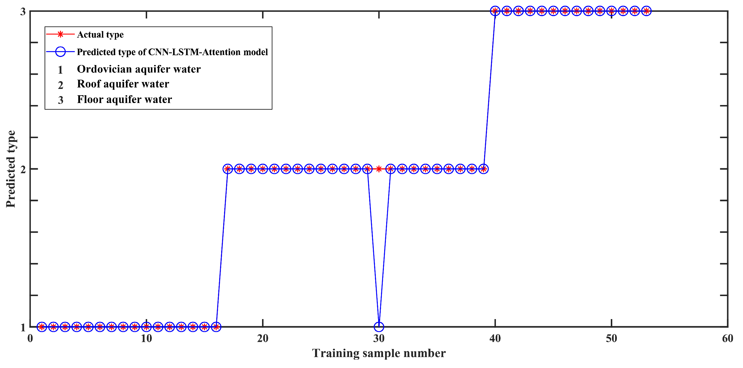Visualizations (Figure 7 and Figure 8) are arranged by class post-training for easier interpretation.

Figure 7 presents the model’s prediction results on the training dataset, showing a misclassification rate of only 2% and a discrimination accuracy of 98%. This demonstrates the model’s strong fitting capacity. However, caution must be exercised to avoid overfitting, where high training accuracy fails to transfer to new data. The quality of predictive models is primarily determined by their performance on unseen samples [62].

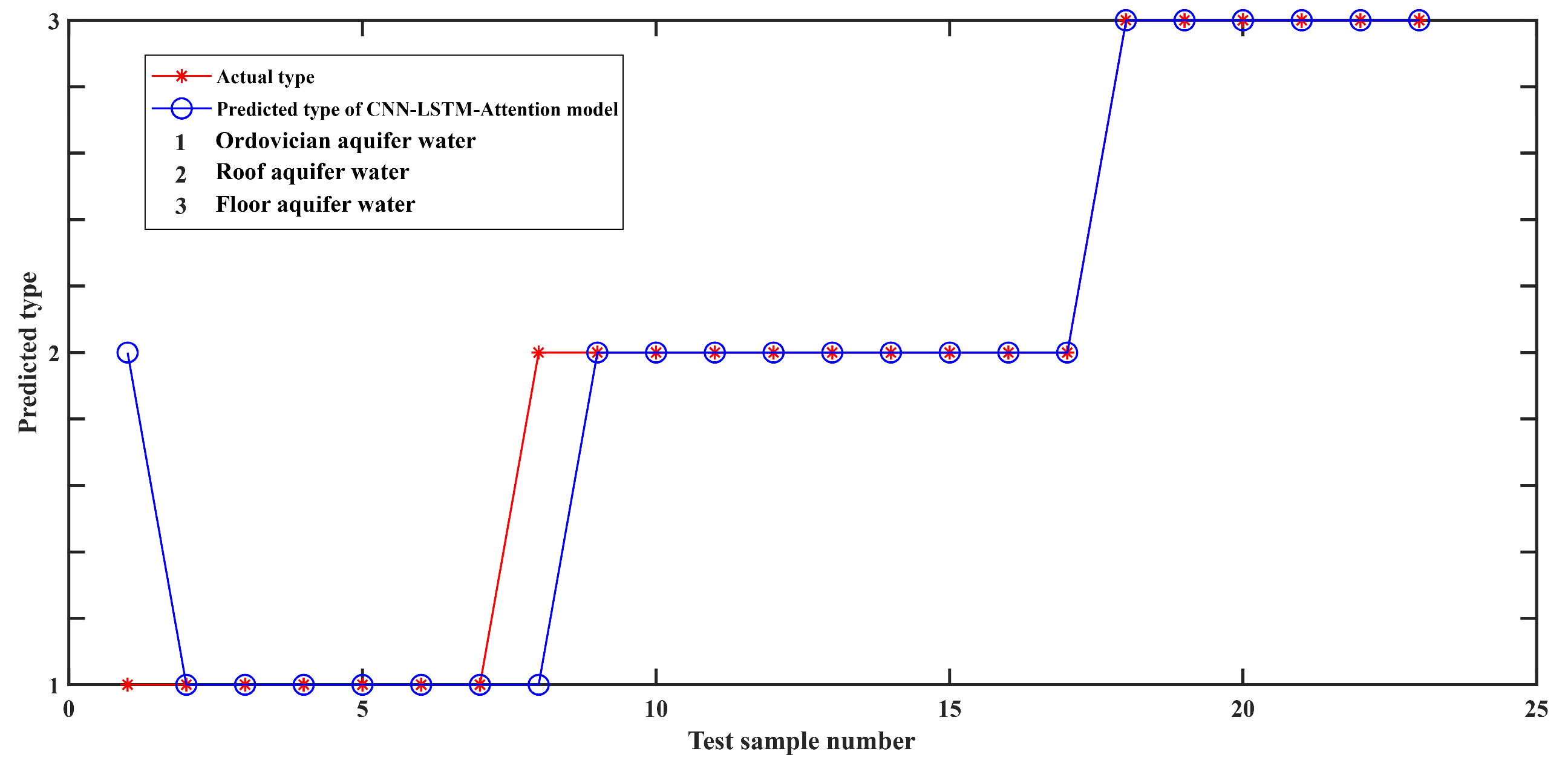
To assess generalization, 23 test samples were employed for validation. As shown in Figure 8, the model achieved a classification accuracy of 91% on test data. Among the three water source types, only one case of roof sandstone aquifer water from the No. 6 coal seam was misclassified as Ordovician limestone aquifer water. The other two aquifer types were always correctly identified. These findings highlight the outstanding performance of the CNN–LSTM–Attention model in identifying mine water inrush sources. The model combines simplicity, low maintenance, and efficiency, achieving high accuracy across both training and test sets.

3.3. Comparative Evaluation of Models

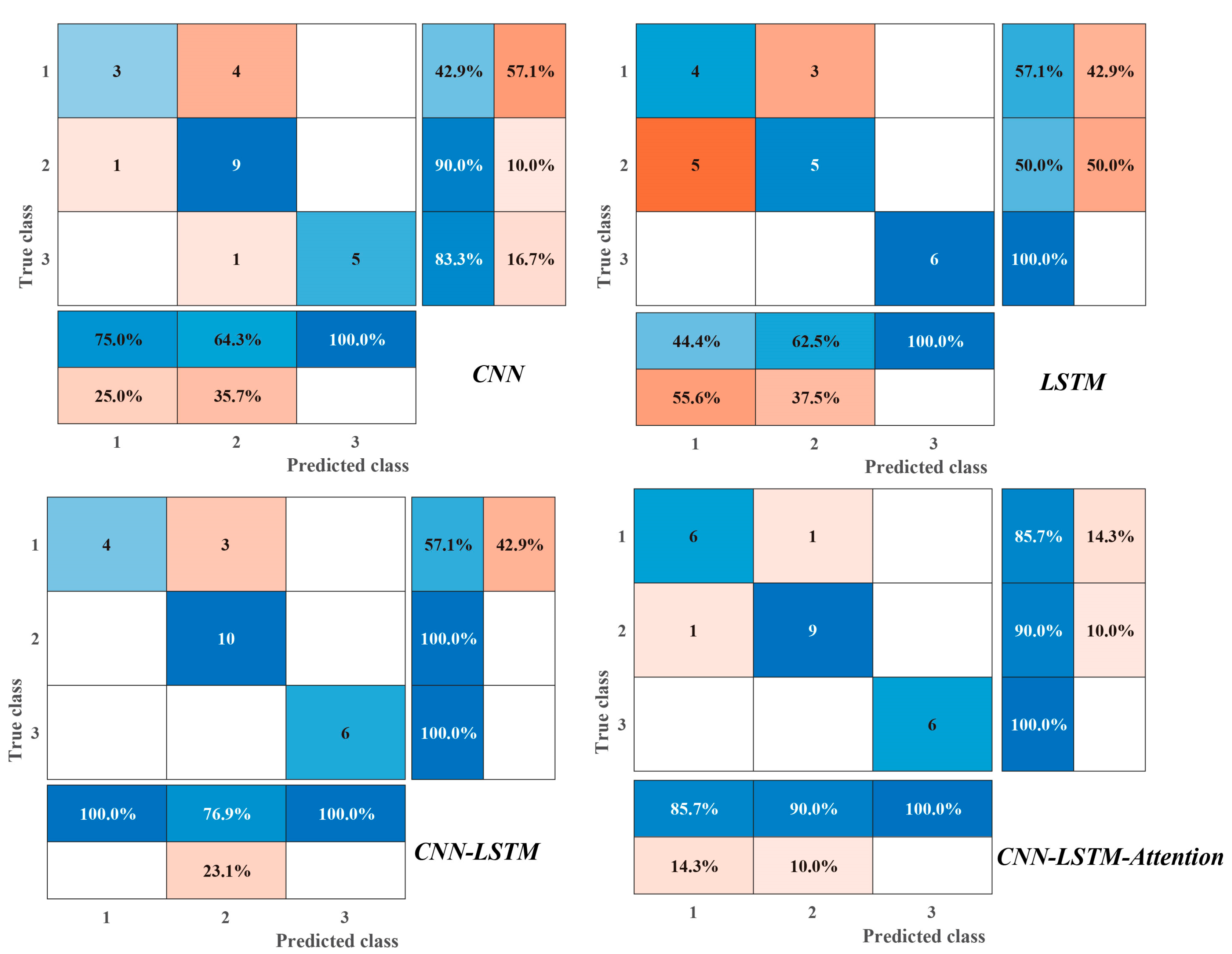
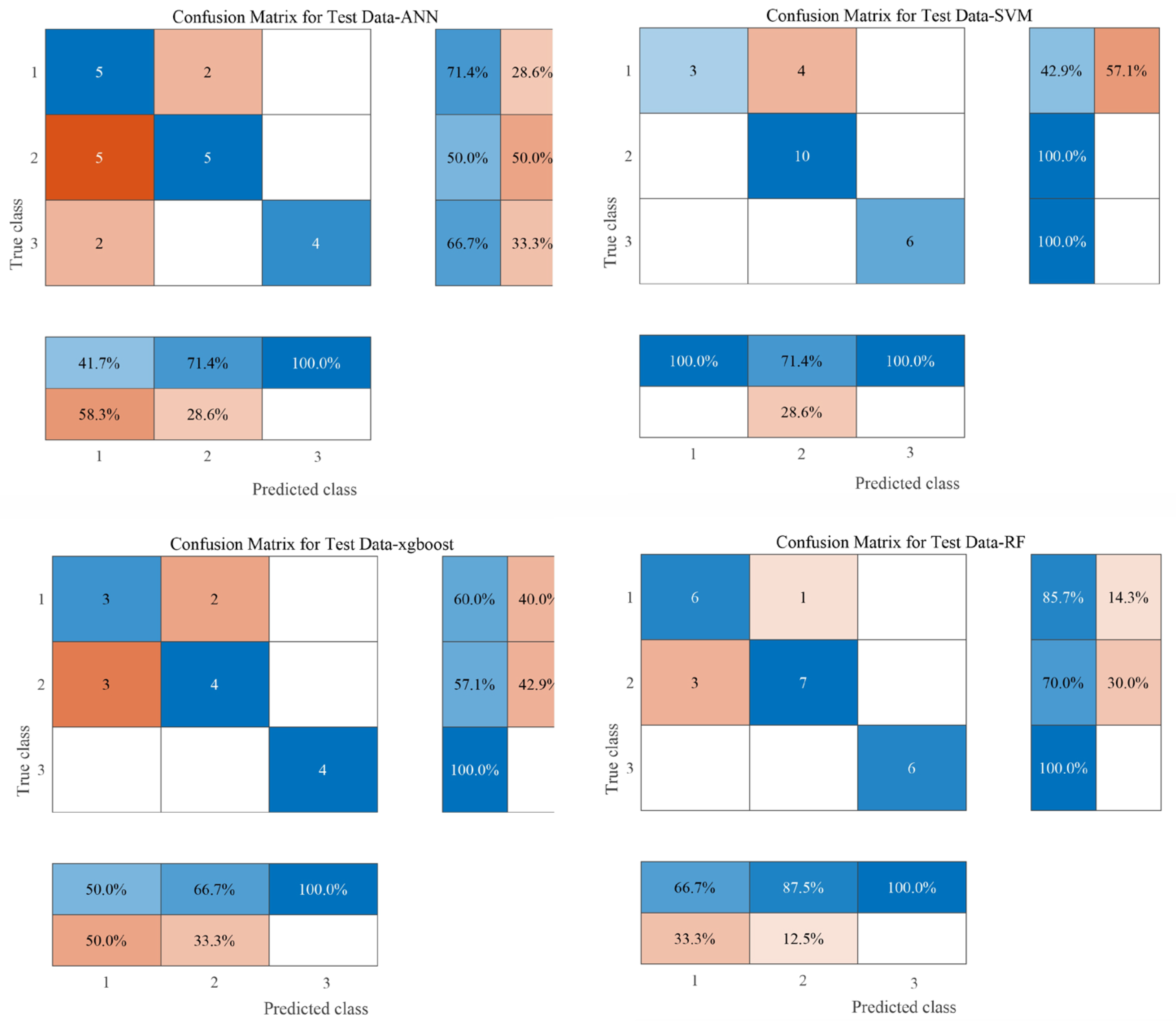
To further evaluate the discrimination performance, an ablation study was conducted by comparing the CNN–LSTM–Attention model with CNN, LSTM, and CNN–LSTM models (Figure 9). The proposed CNN–LSTM–Attention model was evaluated against a suite of established benchmarks in a comprehensive comparative analysis. These benchmarks included the classical machine learning algorithms random forest (RF), support vector machine (SVM), and XGBoost, along with a shallow Artificial Neural Network (ANN) (Figure 10). The results are presented in

Table 3. Comparison of model performance.

Metric	RF	SVM	ANN	XGBoost	CNN	LSTM	CNN–LSTM	CNN–LSTM–Attention
Accuracy	0.826	0.826	0.609	0.688	0.74	0.65	0.87	0.91
Precision	0.847	0.905	0.710	0.722	0.80	0.69	0.92	0.92
Recall	0.852	0.810	0.627	0.724	0.72	0.69	0.86	0.92
F1 Score	0.850	0.855	0.666	0.723	0.76	0.69	0.89	0.92

.

The CNN–LSTM–Attention model achieved an accuracy of 91%, a precision of 92%, a recall of 92%, and an F1 score of 0.92, outperforming all baseline models across all metrics. Specifically, accuracy improved by 27%, 26%, and 4% compared with the CNN, LSTM, and CNN–LSTM models, respectively. The confusion matrices provide a visual comparison of classification outcomes across models, underscoring the superior predictive performance of the proposed framework. Among the classical algorithms, random forest (RF) and support vector machine (SVM) demonstrated the most competitive performance, both achieving an accuracy of 82.6%, F1 scores of 85.0% and 85.5%, respectively. This confirms their capability to learn effective discriminative patterns from the hydrochemical indicators. Notably, SVM achieved the highest precision (90.5%) among all baseline models, but its lower recall (81.0%) compared to RF (85.2%) suggests a tendency to minimize false positives at the cost of missing some true positive identifications. The shallow ANN and XGBoost models performed suboptimally, with accuracies below 70%. This indicates their potential difficulty in capturing the complex, high-dimensional nonlinear relationships within the hydrochemical data, or a propensity for underfitting given the limited sample size.

The deep learning models exhibited a clear performance hierarchy, underscoring the architectural contributions. The standalone LSTM model delivered the weakest performance (65% accuracy), aligning with expectations, as it is not designed for static, spatially oriented feature data. This result highlights the inherent advantage of convolutional operations in extracting local fingerprint features. The CNN model (74% accuracy) significantly outperformed the LSTM by leveraging convolutional kernels to automatically learn local patterns such as ion combinations and ratios. The CNN–LSTM hybrid model marked a substantial performance leap (87% accuracy). This synergy leverages CNN for spatial feature extraction and LSTM to mine potential dynamic evolutionary patterns, validating the merit of incorporating temporal modeling for this task. The proposed CNN–LSTM–Attention model achieved superior performance across the board, attaining the highest accuracy (91%) and F1 score (92%). Crucially, it matched the highest precision (92%) while simultaneously achieving the highest recall (92%), demonstrating a perfectly balanced and robust predictive capability without any significant bias.

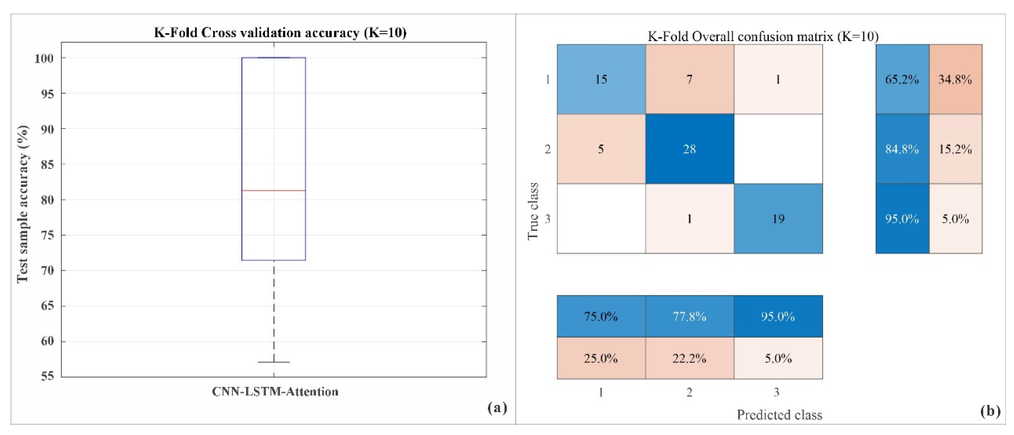
To rigorously evaluate the generalization capability and stability of the proposed CNN–LSTM–Attention model given the limited dataset, a 10-fold cross-validation was conducted. The results, summarized in Figure 11, demonstrate the model’s robust performance.

The distribution of test accuracy across all 10 folds is presented in Figure 11a. The model achieved a median accuracy of approximately 91%, with the interquartile range (IQR) lying between 89% and 93%. The narrow range of accuracy values and the absence of significant outliers indicate that the model’s performance is consistent and not dependent on a particular random split of the data, thus confirming its stability and reliability. The aggregated confusion matrix over all 10 folds, shown in Figure 11b, provides a detailed breakdown of the classification performance for each aquifer type:

(1) Floor aquifer water (Class 3) was identified with the highest precision and recall (95%), with only one instance of being misclassified (as Class 2).

(2) Roof aquifer water (Class 2) was also well-recognized, achieving 84.8% recall, though five samples were confused with Class 1.

(3) Ordovician aquifer water (Class 1) presented the greatest challenge; a recall of 65.2% was achieved. The majority of its misclassifications (7 out of 23 samples) were predicted as Class 2.

This pattern of misclassification suggests a degree of hydrochemical similarity or potential hydraulic connectivity between the roof and floor sandstone aquifers, which is consistent with the geological setting of the study area. The overall high and consistent performance metrics from the cross-validation affirm that the proposed model is not overfitting and possesses strong generalization potential for the task of water inrush source identification.

3.4. Discussion

The CNN model outperforms the LSTM model in discriminating new samples, a phenomenon closely tied to the inherent characteristics of water chemistry data. The water inrush source chemical data (such as ion concentrations) are essentially high-dimensional feature vectors, where the most significant discriminative information often resides in local combinations and ratios between indicators [63,64]. For instance, a high concentration of SO₄²⁻ combined with moderate to high levels of Ca²⁺ and Mg²⁺ is a typical signature of Ordovician limestone aquifer water, while a combination of high Na⁺ + K⁺ with high HCO₃⁻ may indicate coal-bearing sandstone aquifer water. Convolutional kernels in CNNs are naturally designed to capture local feature patterns. Each convolutional kernel acts as a “chemical detector,” automatically scanning all water chemistry indicators to learn local nonlinear combinations, such as “(Ca²⁺ concentration × 0.5 + SO₄²⁻ concentration × 1.2 − HCO₃⁻ concentration × 0.3) > threshold,” that represent the “fingerprint” features of water sources [52]. The CNN does not require prior knowledge of which indicators are important, but instead discovers these discriminative patterns through a data-driven approach. In contrast, standard LSTM models excel at processing temporal dependencies in sequential data (such as contextual information in natural language or time trends in sensor readings). However, in the static data of individual water samples, the temporal dependency is relatively weak. LSTM models must expend additional computational effort to uncover relationships within seemingly “parallel” feature data, making them inherently less efficient than CNNs that specialize in local feature extraction [65].

The CNN-LSTM model shows superior discriminative performance on new samples compared to the CNN model. Although individual water samples are static, forming a water chemistry system [66,67] is a long and dynamic hydrogeochemical process, meaning that the inherent data-generating rules exhibit sequential patterns. Additionally, when constructing training samples, we often aggregate monitoring data from the same water source over different time periods into temporal sequences or construct sequences via technical means that contain valuable dynamic information. The CNN front end performs “dimensionality reduction” and “abstraction,” transforming the raw, potentially redundant water chemistry indicators into a set of higher-level, more discriminative feature maps. This process filters out noise and retains essential features. LSTM receives the refined “high-level feature sequence” produced by the CNN, rather than the raw data. The advantage of LSTM lies in its ability to extract deeper, more complex nonlinear dynamic evolution patterns from these high-level feature sequences. For example, the model may learn that “Feature A rises then falls, while Feature B steadily increases” is a typical evolutionary path for a particular water source. The CNN–LSTM architecture achieves a perfect division of labor: CNN “sees” the microscopic chemical features, while LSTM “understands” the macroscopic evolution of these feature combinations. This synergy of “spatial feature extraction” and “temporal relationship modeling” enables the model to extract more information from the data, thus surpassing the performance of a single model.

The CNN–LSTM–Attention model achieves a significant improvement in discriminating new samples compared to the CNN–LSTM model [68,69]. The introduction of the attention mechanism greatly enhances the model’s performance, marking the most critical and innovative aspect of the model. A standard CNN–LSTM model assumes equal contributions from all time steps (and all feature points) when processing sequences. However, this assumption does not align with geochemical principles in water source identification, where certain indicators are more indicative than others. The advantages of the attention mechanism are as follows:

Feature importance weighting (focusing on key information): The attention mechanism allows the model to selectively focus on the most discriminative feature moments during the final decision-making process [70,71]. For instance, the model can learn to assign high weights to features representing “SO₄²⁻ concentration” and “Sr²⁺ trace elements”, while assigning lower weights to indicators like “pH,” which is more susceptible to environmental interference. This is akin to an expert focusing on a few key indicators when reviewing a chemical analysis, rather than considering each data point equally.

Dynamic adaptive discrimination: The critical discriminative indicators vary across different water sources. The attention mechanism equips the model with dynamic adaptability, automatically focusing on key indicators when handling different types of water sources [72,73,74]. For example, when processing a suspected Ordovician limestone aquifer sample, the model will focus on SO₄²⁻ and Ca²⁺, while for a suspected Quaternary pore water sample it may prioritize TDS and Cl⁻ concentrations. This flexibility is unattainable with models that rely on fixed parameters.

Enhanced robustness and interpretability: By ignoring irrelevant or noisy information, the attention mechanism greatly improves the model’s robustness in dealing with complex, real-world data [75]. Furthermore, the generated attention weight maps provide strong interpretability. We can visualize which indicators the model focuses on when classifying a sample, ensuring these align with current hydrogeochemical understanding. This makes the model less of a “black box”, enhancing the reliability and persuasiveness of the conclusions.

The introduction of the attention mechanism elevates the model from a paradigm of “uniform treatment of all information” to an intelligent discriminative paradigm that mimics expert thinking, focusing on the most important features while ignoring less significant ones. This is not merely a performance improvement; it represents an evolution in the model’s discriminative philosophy, improving alignment with practical applications.

The CNN–LSTM–Attention model successfully integrates these three advantages: it uses CNN to capture chemical fingerprints, LSTM to uncover evolutionary patterns, and the attention mechanism to emulate expert decision-making by focusing on core evidence. This architecture allows the model to make more accurate, robust, and trustworthy distinctions when faced with complex, high-dimensional, and noisy water chemistry data, which is the fundamental reason for its exceptional performance in the ablation study. A post hoc analysis using Shapley Additive Explanations (SHAP) was conducted to rigorously validate the global feature importance. A summary plot (Figure 12) reveals that the Ca²⁺ concentration is, by a considerable margin, the most impactful feature for the model’s predictions, exhibiting the highest mean absolute SHAP value. The Mg²⁺ concentration is the second most important feature. The prominence of calcium and magnesium observed here aligns with fundamental hydrogeochemical principles, as their abundance is a primary indicator of water–rock interactions, particularly interactions involving the carbonate minerals (e.g., calcite, dolomite) prevalent in many aquifer systems. Cl⁻ and SO₄²⁻ ions show a moderate but significant influence. Notably, the distribution of points indicates that higher values of Ca²⁺ and Mg²⁺ (red points) have a positive impact on the model output (positive SHAP values), pushing the prediction towards a certain class. Conversely, higher concentrations of Cl⁻ and SO₄²⁻ generally exhibit a negative impact (negative SHAP values), suggesting a different hydrochemical facies. The K⁺/Na⁺ and HCO₃⁻ ions exhibited the lowest overall influence on the model’s decisions in this context of this study. This SHAP-based interpretation provides a validated, quantitative ranking of feature importance, which will be cross-referenced with the attention mechanism in the following discussion.

Piper trilinear diagrams are a classic tool for hydrochemical source identification. They classify water types by plotting the relative contents of major cations (Ca²⁺, Mg²⁺, Na⁺+K⁺) and anions (Cl⁻, SO₄²⁻, HCO₃⁻) in triangular coordinate systems, thereby distinguishing aquifer types based on clustering patterns. The CNN–LSTM–Attention model achieved 91% accuracy on the test set, with precise classification of three aquifer types (RW, FW, OW). This is consistent with the clustering results of Piper diagrams (Figure 13). For instance, OW samples, which are typically clustered in the SO₄²⁻-Ca²⁺ dominant region in Piper diagrams, were correctly identified by the model (high recall). The few misclassifications (e.g., individual RW samples misclassified as OW) also align with the overlapping hydrochemical regions of similar aquifers in Piper diagrams, reflecting actual geological connectivity rather than model errors. Piper diagrams rely heavily on manual interpretation and struggle with ambiguous signatures or mixed water samples. In contrast, the model’s attention mechanism automatically weights key ions (e.g., SO₄²⁻ with the highest SHAP value), effectively resolving the overlapping clusters in Piper diagrams and improving classification accuracy for mixed samples.

Ionic ratio methods (e.g., Ca²⁺/Mg²⁺, Cl⁻/HCO₃⁻) reflect water–rock interaction processes and aquifer properties by analyzing the proportional relationships between ions. For example, a high Ca²⁺/SO₄²⁻ ratio is indicative of limestone aquifers, while a high Na⁺/Cl⁻ ratio may suggest silicate weathering in sandstone aquifers. The model’s attention weights and SHAP value analysis confirm its recognition of geochemically meaningful ionic ratios. For example, SO₄²⁻ and Ca²⁺, which are critical in ionic-ratio-based OW identification, were identified by the model as the top two influential features. This consistency verifies that the model’s classifications are rooted in actual ionic ratio relationships rather than statistical noise. Traditional ionic ratio methods often focus on a limited number of ratios, leading to incomplete feature extraction. The CNN–LSTM–Attention model, via a 1D-CNN, automatically extracts complex nonlinear combinations of multiple ionic ratios (e.g., (Ca²⁺ × 0.5 + SO₄²⁻ × 1.2 − HCO₃⁻ × 0.3)), integrating multi-dimensional ratio information to capture more subtle geochemical differences between aquifers.

4. Conclusions

In this study, we addressed the problem of identifying water inrush sources in coal mines by developing a deep learning fusion model based on CNN–LSTM–Attention. The model integrates convolutional neural networks to extract the local features of hydrochemical data, long short-term memory networks to capture temporal dependencies, and an attention mechanism to adaptively focus on key discriminative indicators. The main conclusions are as follows:

(1) The proposed CNN–LSTM–Attention fusion model demonstrated exceptional performance in identifying water inrush sources in the Tangjiahui Coal Mine, achieving a test accuracy of 91%, surpassing both traditional machine learning and other deep learning benchmarks. This confirms the model’s superior ability in handling complex, high-dimensional hydrochemical data.

(2) The model’s architecture successfully integrates the strengths of its components: a CNN for extracting local hydrochemical fingerprints, LSTM for modeling potential dynamic evolutionary patterns, and an attention mechanism for providing interpretable, weighted decision-making. This synergistic design enables a comprehensive analysis beyond static snapshots.

(3) The model offers significant transparency. The visualization of attention weights, validated by SHAP analysis, revealed that its decisions are based on key discriminative ions (e.g., Ca²⁺, Mg²⁺), aligning with established hydrogeochemical principles. This greatly enhances the trustworthiness and practical utility of the model.

In terms of applicability, while the specific trained model is inherently calibrated to the hydrogeochemical conditions of the Tangjiahui Mine and thus its direct application to other sites is limited, the methodological framework used to develop the model is highly generalizable. The core approach of feature extraction, temporal modeling, and interpretable classification provides a powerful and transferable blueprint for intelligent water source identification in other mining regions with similar challenges. The primary limitation of this methodology is the site-specific nature of the training dataset. Therefore, future work will focus on expanding the dataset to encompass multiple mining districts, incorporating additional geochemical tracers into the model (e.g., isotopes), and explicitly implementing transfer learning techniques to enhance the model’s cross-site adaptability and robustness, thereby fully realizing its potential as a universal tool for mine water hazard prevention.