Abstract
Data-driven fault location methods based on deep learning offer strong feature learning and nonlinear mapping capabilities; however, in low-voltage distribution grids (LVDG) the scarcity of high-rate sampling devices and the variability introduced by distributed renewable generation lead to data insufficiency and data imbalance, which reduce the accuracy of deep-learning-based fault location. To address this, this paper proposes an adaptive working condition-based fault location method that integrates S-transform-enhanced feature extraction with progressive transfer learning. The method clusters working conditions using k-means on a 21-dimensional indicator set covering load, photovoltaic, and voltage. For each condition, a CNN is trained on the corresponding data, and the S-transform extracts distinctive time-frequency signatures from limited measurements to separate fault points at similar distances from the feeder head. Then, progressive transfer learning with Euclidean distance-based domain adaptation migrates effective parameters from data-rich conditions to data-scarce ones through fine-tuning and medium-tuning, thereby addressing the degradation of fault-location accuracy in scenarios with limited data. Experimental validation on a 400 V LVDG demonstrates superior performance, achieving 99.80% fault location accuracy and 99.72% fault type classification. The S-transform enhancement improves fault location by 6.63%, while transfer learning maintains 96% accuracy in edge conditions using only 200 samples.
1. Introduction
1.1. Research Motivation
Low-voltage distribution grids (LVDGs) serve as the backbone of modern electrical distribution systems, forming the final link in the delivery of power to end-users. The growing integration of renewable energy sources (RES)—such as photovoltaic (PV) systems—has introduced increased complexity into LVDG operation [1,2]. This evolution underscores the critical importance of efficient and accurate fault location techniques to ensure grid reliability. Precise fault identification and location are essential for reducing outage durations, optimizing maintenance strategies, and enhancing overall system resilience, particularly as decentralized generation makes grid behavior more variable and less predictable.
Traditional fault location techniques, such as impedance-based and traveling-wave methods [3,4], exhibit notable shortcomings when applied to LVDGs. They were devised for transmission systems and struggle with low fault impedances, multi-branch topologies, short propagation paths, high-frequency attenuation, and dependence on predetermined network parameters [5]. These constraints motivate the shift to data-driven approaches. However, for LVDGs, current data-driven fault location techniques still face two persistent issues: (i) dependence on sufficiently rich sampled data to extract discriminative features, which is difficult in LVDGs lacking sufficient sampling infrastructure, and (ii) high sensitivity to distribution imbalance, so rare or extreme working conditions are underrepresented and model accuracy declines in these scenarios.
In summary, there is an urgent need for an improved data-driven method that achieves accurate LVDG fault location under sparse sampling conditions and imbalanced operating-condition distributions. Therefore, this paper proposes transforming limited sampled data with the S-transform into time-frequency-energy representations that capture richer frequency-dependent energy concentration and attenuation patterns during fault propagation, thereby enabling precise fault location under limited data. Then, year-round LVDG working conditions are clustered and a data-driven model is trained on data-rich regimes. Transfer learning is applied to migrate the learned parameters to data-scarce regimes, achieving robust accuracy in rare scenarios and mitigating the impact of distribution imbalance.
1.2. Related Work
The limitations of conventional fault location techniques have driven extensive research into alternative methodologies. Data-driven approaches, typified by machine learning (ML), have attracted increasing attention in recent years. Early ML applications focused on pattern recognition techniques, with neural networks being among the first to show promise in fault classification tasks [6]. Subsequently, methods such as support vector machines (SVM) [7], random forest model [8], and k-nearest neighbors (k-NN) [9] have been applied to fault location with moderate success. More recent advances have explored deep learning architectures, with Rizeakos V et al. [10] pioneering the application of deep neural networks to fault location in distribution systems, achieving accuracy improvements of 10–20% over traditional methods. More recently, convolutional neural networks (CNNs) have demonstrated strong potential due to their ability to automatically extract discriminative features from raw and noisy input data [11]. However, related studies [12,13] reveal that while CNNs excel at feature extraction, their performance is highly dependent on training data quality and quantity.
Regarding training data quality, LVDG fault location suffers from insufficient sampling features in practical settings. While studies on medium-voltage distribution networks often assume high-density sampling infrastructure at critical nodes [14], the typical LVDG architecture is radial with numerous end-user connections and limited sampling infrastructure, fundamentally constraining data availability and feature richness. In practice, infrastructure costs and communication constraints concentrate high-rate sensing at the substation/head-end, with only sparse or low-rate measurements downstream, which limits discriminative feature extraction for data-driven models. Refs. [15,16] explored economical alternatives that leverage smart meters/AMI to support fault location, acknowledging that dense μPMU deployment is often impractical at LV scale. However, AMI/smart meters typically record at 5/15 min intervals, which is far from the millisecond-scale waveform sampling needed for fault localization, so these data are not directly applicable to high-speed fault-location tasks [17,18]. This cost and infrastructure reality aligns with practice, as devices often prioritize cost and size reduction [19] and many industrial monitoring tasks operate on second level cycles rather than milliseconds [20]. Therefore, CNN models that rely on abundant data must be adapted by extracting richer features from limited datasets so they better meet practical application needs, including distinguishing similar faults under sparse measurements.
Regarding training data quantity, the volatility of RES makes the proportions of working conditions in historical datasets highly uneven [21], and some extreme scenarios contain very little data for fault location. For data-dependent CNN-based methods, this challenge is particularly acute [22]. ML models in safety critical domains underscore the need to maintain reliability and interpretability under limited data and shifting working conditions [23,24]. RES stochasticity causes fluctuations in load, generation, and voltage, yielding diverse and dynamic working conditions [25,26]. These working conditions are unevenly represented in historical datasets, with rare or extreme states severely under-sampled due to a fundamental mismatch between model assumptions and actual working conditions [27,28]. Consequently, standard ML training procedures, which optimize for average performance across all samples, systematically underrepresent these conditions during model training, as optimization algorithms naturally prioritize the dominant patterns corresponding to normal or common operating states. In recent power system studies, ref. [29] proposes a data mining based fuzzy classification E algorithm tailored to imbalanced distribution fault data, mitigating bias toward dominant regimes; ref. [30] introduces hierarchical GAN based augmentation to synthesize minority condition samples and improve generalization when labeled waveforms are scarce. However, these approaches can introduce errors during data synthesis and modification, including distribution distortions and label noise, which may reduce overall data quality and degrade ML model performance. In this context, transfer learning can migrate effective model parameters from data-rich working conditions to data-scarce ones, improving robustness and accuracy in rare scenarios.
To better position our contribution, Table 1 provides a concise comparison between representative ML- and CNN-based fault-location approaches and the proposed method. The comparison summarizes key criteria, including the type of features used, dependence on measurement infrastructure, use of transfer or augmentation techniques, and real-time feasibility. As shown in Table 1, most prior studies rely on dense measurement points or abundant labeled data, whereas our approach achieves high accuracy with only feeder-head sensing and progressively transferred CNN models built upon S-transform features.

Table 1.
Comparison of representative fault-location approaches with the proposed method.
1.3. Summary of Contributions
To address the above limitations in training data quantity and quality, and contribute toward fault location capabilities in LVDGs, this work proposes an adaptive working condition-based fault location method for LVDGs using progressive transfer learning and time-frequency analysis. The proposed approach specifically targets the challenges of sample scarcity in diverse working conditions and limited sampling infrastructure that characterize real-world LVDG deployments. By leveraging time-frequency analysis and domain adaptation techniques, this method enables reliable fault location under varying RES conditions while maintaining computational efficiency suitable for real-time applications.
The main contributions of this work can be concisely described as follows:
- Development of a novel working condition-adaptive framework. Built on a 21-dimensional condition descriptor, the framework clusters year-round operating states and routes data to condition-specific CNNs. This framework reduces distribution imbalance by separating data-rich and data-scarce conditions, supports targeted training with matched-condition inference, and lays the groundwork for transfer learning between conditions.
- Proposal of an S-transform–enhanced feature extraction methodology. This method adopts the S-transform to extract time–frequency–energy features from voltage and current data collected by limited sampling devices, capturing frequency-dependent energy concentration and attenuation during fault propagation, thereby achieving reliable discrimination of fault points under sparse sensing.
- Proposal of a progressive transfer learning strategy. The proposed strategy addresses sample scarcity in extreme working scenarios through Euclidean distance-based domain adaptation, enabling effective model generalization from data-rich dominant conditions to data-scarce edge conditions with significantly reduced training requirements and faster convergence.
The remainder of this paper is organized as follows: Section 2 formulates the problem by analyzing LVDG system characteristics, fault characteristics, and working condition variability. Section 3 details the proposed working condition-adaptive framework. Section 4 presents the S-transform enhanced feature extraction approach for distinguishing similar faults under sparse measurements. Section 5 introduces the progressive transfer learning strategy for edge condition adaptation. Section 6 provides comprehensive experimental validation. Finally, Section 7 concludes with key findings and future research directions.
2. Problem Statement and Condition-Adaptive Framework
This section comprehensively analyzes the fault location challenges in LVDG and establishes a process for the proposed method based on adaptive working conditions. The content includes three key aspects: the inherent structure and measurement limitations of the LVDG, the statistical characteristics of working condition changes throughout the operational period, and the framework process for adaptive fault location in different working conditions.
2.1. LVDG System Characteristics and Infrastructure Constraints
LVDGs are typically configured as radial networks with extensive branching paths that supply a large number of end-users. These systems serve thousands of residential, commercial, and small-industrial customers through distribution transformers that interface directly with user-side meters. Unlike transmission and medium-voltage systems, which are generally equipped with comprehensive monitoring infrastructure, LVDGs face significant limitations in measurement deployment due to economic constraints and misaligned business needs. These limitations fundamentally impair fault location accuracy and overall system observability.
In practical LVDG deployments, the effective sampling infrastructure exhibits a pronounced concentration bias toward feeder head-end locations, where high-precision smart meters and integrated smart terminal (ICT) devices are typically installed. As illustrated in Figure 1, real-time sensing is concentrated at the substation/feeder head-end, where an ICT, a dedicated high-frequency sampling device, can reach a sampling frequency of 200 samples per second. In contrast, most downstream nodes are equipped only with basic meters and provide low-rate readings at 5/15 min intervals, which are unsuitable for ML-based (e.g., CNN) fault-location models. This deployment pattern is primarily cost-driven. Centralized monitoring at the substation reduces installation and maintenance effort, and aggregated load profiles still satisfy customer-side billing requirements. However, these limitations result in large portions of the grid infrastructure having no real-time monitoring capability, forcing fault detection and location to rely exclusively on information obtained from a limited number of feeder head-end measurement points. A major challenge arising from this setup is that faults occurring at different locations within the same feeder segment often produce nearly identical voltage and current signatures at the feeder head-end. For example, faults at electrically similar distances from the measurement point yield highly comparable waveforms, a situation where conventional amplitude-based analysis methods fail to provide sufficient discrimination. Accordingly, we use the S-transform to extract time-frequency-energy features from head-end data, capturing richer frequency-dependent energy concentration and attenuation patterns as faults propagate toward the head-end and thereby enabling precise fault-location determination, as detailed in the subsequent sections.
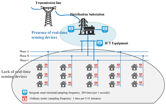
Figure 1.
Typical LVDG Structure and limitations of measurement capability. The measurement capability is concentrated in substations, leaving most of the LVDG unmonitored.
2.2. Working Condition Variability and Data Distribution Characteristics
The integration of RES, especially distributed photovoltaic, has significantly increased operational variability and uncertainty in LVDG. These dynamic conditions challenge the reliability of fault location algorithms, as active LVDG exhibit unpredictable load and generation patterns that complicate the detection and analysis of fault signatures.
For instance, the variability of photovoltaic output across different seasons and months significantly influences voltage profiles along the distribution feeder. Higher generation in summer can cause sustained overvoltage conditions, while lower output in winter leads to reduced voltage levels. These variations alter the magnitude and phase angle of voltage and current signals measured at the feeder head-end. Consequently, fault-induced changes become less distinguishable from normal fluctuations caused by PV generation variability, thereby reducing the reliability of fault detection and the accuracy of location estimation.
Moreover, the inherent imbalance in historical measurement data poses significant challenges to developing reliable fault location methods, particularly for machine learning-based approaches [31]. For instance, critical scenarios—such as extreme weather or high distributed energy resource variability—are typically underrepresented in historical datasets, accounting for less than 3% of training samples. Consequently, standard ML training procedures tend to prioritize frequently occurring patterns during optimization, leading to systematically poor representation of these rare but critical conditions in the resulting models.
Therefore, performing a year-round clustering analysis of LVDG working conditions is highly meaningful. On one hand, it enables the identification and explicit modeling of these underrepresented yet critical scenarios. On the other hand, it provides a statistical foundation for developing adaptive fault location strategies that can maintain accuracy across both common and rare operating states.
2.3. Working Condition-Adaptive Framework Requirements
Building upon the critical challenges identified in the preceding analysis, specifically the need for advanced signal processing techniques to extract discriminative features from limited measurement points and the necessity of working condition analysis to mitigate data imbalance issues, this section proposes an adaptive working condition-based fault location framework for reliable fault location in low-voltage distribution grids under diverse working conditions.
The proposed framework consists of four main processes, as illustrated in Figure 2.

Figure 2.
Flowchart of the proposed adaptive working condition-based fault location framework.
Process 1: Working Condition Clustering (Offline Phase). The framework begins with clustering analysis of year-round load-photovoltaic operational data using 21-dimensional features. K-means clustering is employed to identify multiple distinct working conditions based on comprehensive system characteristics. Subsequently, these identified conditions are categorized by sample size into dominant condition, regular condition, and edge conditions, establishing a hierarchical working condition database that systematically addresses data imbalance challenges in LVDG fault location. In addition, centroids of all clusters are retained, and the centroid of the dominant condition is designated as the reference for computing inter-condition similarity.
Process 2: S-Transform Enhanced CNN Training (Offline Phase). Following clustering, the framework proceeds to CNN model training, initially focusing on the dominant working condition cluster where sample abundance ensures robust feature learning. The key innovation here is the integration of S-transform processing for voltage and current amplitude signals collected at feeder head-end locations. This time-frequency analysis extracts high-resolution spectral-temporal characteristics that reveal subtle fault signatures otherwise masked in conventional amplitude-based measurements. The S-transform enhancement directly addresses the observability challenges posed by limited sampling infrastructure, enabling the CNN to distinguish between similar fault points that produce nearly identical amplitude signatures.
Process 3: Progressive Transfer Learning (Offline Phase). The third process implements progressive transfer learning to extend the well-trained dominant condition model to sample-scarce scenarios. Using Euclidean distance metrics in the feature space, the framework employs two adaptation strategies: fine-tuning for regular conditions and medium-tuning for edge conditions. This systematic knowledge transfer from the sample-rich dominant condition model enables effective model adaptation without requiring extensive training data for every operational scenario. The process ensures that even edge conditions—representing less than 3% of historical samples—achieve acceptable fault location accuracy.
Process 4: Real-time Fault Location (Online Phase). During online application, the framework executes a two-stage adaptive process for incoming fault events. Stage 1 performs rapid working condition recognition by matching the current 21-dimensional feature vector against pre-established clusters. Stage 2 then deploys the corresponding condition-specific CNN model from the repository for precise fault location.
3. Multi-Dimensional Working Condition Clustering
To address the challenge of diverse working conditions in LVDG with high PV penetration, this section presents a comprehensive working condition clustering method that systematically categorizes operational states based on multi-dimensional features extracted from year-round historical data.
3.1. Feature Model for Working Condition Characterization
The proposed clustering framework begins with the construction of a 21-dimensional feature space that comprehensively captures the operational characteristics of the LVDG throughout the year.
3.1.1. Load Feature
Seven features are extracted to characterize load variation patterns:
- ➀
- The normalized load at time t is computed as
The corresponds to the value of feature 1 at time t. Here, represents the total LVDG load at time t, while and denote the annual minimum and maximum load values, respectively.
- ➁
- The 24 h moving average load at time t is computed as
The corresponds to the value of feature 2 at time t. Here, represents the total LVDG load at time i.
- ➂
- Load variability is captured through the 24 h standard deviation:
The corresponds to the value of feature 3 at time t.
- ➃
- Peak load tracking within the 24 h window is computed as
The corresponds to the value of feature 4 at thime t.
- ➄
- The ratio of the load value in the LVDG at time t to the maximum load over the past 24 h is computed as
The corresponds to the value of feature 5 at time t.
- ➅
- The ratio of the load value in the LVDG at time t to the average load over the past 24 h is computed as
The corresponds to the value of feature 6 at time t.
- ➆
- The deviation between the load value in the LVDG at time t and the average load over the past 24 h is computed as
The corresponds to the value of feature 7 at time t.
3.1.2. Photovoltaic Generation Feature
Four features characterize PV generation variation patterns:
- ➀
- The normalized PV output at time t is computed as
The corresponds to the value of feature 8 at time t. Here, represents PV output at time t, while and denote the annual minimum and maximum PV output values, respectively.
- ➁
- The average PV output value over the past 24 h at time t is computed as
The corresponds to the value of feature 9 at time t. Here, represents PV output at time i.
- ➂
- The PV output value variability is characterized by its 24 h standard deviation is computed as
The corresponds to the value of feature 10 at time t.
- ➃
- The PV-load balance value at time t is computed as
The corresponds to the value of feature 11 at time t.
3.1.3. Voltage Feature
Eight features capture voltage characteristics across the network:
- ➀
- The minimum voltage value in the LVDG at time t is computed as
The represents the value of feature 12 at time t. denotes the voltage magnitude at bus b, serves as the index symbol for buses in the LVDG, indicating that b belongs to an arbitrary bus within the network.
- ➁
- The maximum voltage value in the LVDG at time t is computed as
The corresponds to the value of feature 13 at time t.
- ➂
- The average voltage value in the LVDG at time t is computed as
The corresponds to the value of feature 14 at time t.
- ➃
- The standard deviation of voltage in the LVDG at time t is computed as
The corresponds to the value of feature 15 at time t.
- ➄
- The average voltage deviation rate in the LVDG at time t is computed as
The corresponds to the value of feature 16 at time t.
- ➅
- The number of low-voltage nodes in the low-voltage distribution grid at time t is computed as
The corresponds to the value of feature 176 at time t. Here, denotes an indicator function such that if the condition is satisfied, and otherwise.
- ➆
- The deviation between the load value in the LVDG at time t and the average load over the past 24 h is computed as
The corresponds to the value of feature 18 at time t.
- ➇
- The voltage unbalance degree in the low-voltage distribution grid at time t is computed as
The corresponds to the value of feature 19 at time t.
3.1.4. Temporal Encoding Features
Two cyclical features encode temporal patterns:
- ➀
- The sine-encoded value at time t is computed as
The represents the value of feature 20 at time t.
- ➁
- The cosine-encoded value at time t is computed as
The corresponds to the value of feature 21 at time t.
The above 21-dimensional feature set comprehensively captures the operating characteristics of LVDG through multi-scale temporal analysis and cross-domain correlation. These features, spanning load patterns (7 features), photovoltaic generation variability (4 features), voltage characteristics (8 features), and temporal encoding (2 features), enable characterization of diverse working conditions throughout the year. The feature model constructs a comprehensive 8760 × 21 feature matrix that serves as the foundation for subsequent clustering analysis and condition-based fault location.
3.2. Working Condition Clustering by K-Means
3.2.1. Feature Normalization
Prior to clustering analysis, the 21-dimensional feature matrix undergoes standardization processing to ensure equal weighting across different feature scales. The first 19 continuous features are normalized using Z-score standardization, and the model is as follows:
where represents the i-th feature, and denote the mean and standard deviation of feature i across all time instances. The temporal encoding features (features 20–21) are already bounded within [−1, 1] due to their sinusoidal nature and require no additional normalization.
3.2.2. K-Means Clustering Implementation
K-means is adopted due to its computational efficiency with year-long datasets, straightforward implementation requiring only the number of clusters (k) as a parameter, and reproducible results. Furthermore, its centroid-based framework is compatible with the Euclidean distance metric employed in subsequent analysis and supports the proposed progressive transfer learning approach. The specific procedure is as follows: the K-means clustering algorithm is applied to the standardized 8760 × 21 feature matrix to identify distinct working conditions. The clustering process iteratively assigns each hourly sample to the nearest cluster centroid and updates centroids until convergence. The specific model is as follows:
where denotes the number of clusters, represents the 21-dimensional feature vector at hour i, and is the centroid of cluster k.
To determine the optimal number of the K-means clustering algorithm, the Silhouette Coefficient is computed for different cluster numbers ranging from 2 to 10:
where represents the mean intra-cluster distance and denotes the mean nearest-cluster distance. The optimal cluster number K* is selected as
Through the above analysis, the clustering algorithm establishes a comprehensive working condition repository that captures the full spectrum of LVDG working conditions throughout the year.
3.3. Working Condition Recognition and Adaptive Model Selection
3.3.1. Working Condition Classification
Following the clustering analysis, the identified working conditions are classified into three categories based on sample distribution and the number of samples they contain:
- Dominant Working Condition. The cluster with the largest number of samples, representing the most frequent working conditions.
- Regular Working Conditions. Clusters with moderate sample sizes, capturing common but less frequent working conditions.
- Edge Working Conditions. Clusters with the smallest sample sizes, representing rare but critical working conditions such as extreme weather events or unusual RES fluctuations.
3.3.2. Condition-Specific Model Training
For each identified working condition, a dedicated CNN model is trained using the corresponding subset of fault scenarios. The dominant working condition, with its abundant training samples, serves as the foundation for developing the base CNN model. These base CNNs are capable of accurate fault type identification and location estimation through S-transform-enhanced feature extraction. The knowledge acquired by these base CNNs is then transferred to other working conditions via the transfer learning strategy detailed in Section 5, enabling effective adaptation even in data-scarce conditions.
3.3.3. Online Adaptive CNN Model Selection
During real-time operation, the method implements a two-stage adaptive fault location process:
- Stage 1—Working Condition Recognition. When a fault event occurs, the system extracts the current 21-dimensional feature vector and performs rapid condition matching using K-nearest neighbor classification:where represents the operational characteristics of the current fault event, denotes the centroid of working condition c, and is the index of the working condition cluster that best matches the current fault event.
- Stage 2—Condition-Specific CNN Model Selection. Based on the identified working condition, the process of condition-specific CNN model selection deploys the corresponding pre-trained CNN model from the condition-specific model repository. This ensures that fault location is performed using a model optimized for the current fault event, significantly improving localization accuracy across diverse grid working conditions.
Thus, the adaptive framework enables robust fault location across the full spectrum of LVDG working conditions, from frequent dominant conditions to rare but critical edge conditions.
4. S-Transform Enhanced Feature Extraction
The limitation of sparse sampling infrastructure in LVDG creates significant challenges for fault location accuracy, particularly when faults occurring at different locations produce nearly identical amplitude signatures at feeder head-end measurement points. To address this problem, this section presents a S-transform-based time-frequency analysis method that extracts spectral-temporal characteristics from limited sensing infrastructure and utilizes them as inputs to a subsequent CNN.
4.1. Signal Preprocessing and Normalization
Signal preprocessing ensures consistent feature scaling across different measurement points throughout the LVDG network. The preprocessing pipeline begins with amplitude normalization to eliminate bias introduced by varying measurement scales and system operating points.
For voltage measurements at bus b, the normalization process is expressed as
where represents the instantaneous voltage amplitude, denotes the mean over the analysis window, and signifies the standard deviation over the analysis window.
Similarly, current signal normalization follows:
where represents the instantaneous current amplitude, denotes the mean over the analysis window, and signifies the standard deviation over the analysis window.
The above normalization ensures that subsequent S-transform analysis operates on signals with zero mean and unit variance, facilitating consistent feature extraction across diverse working conditions and measurement locations.
4.2. S-Transform Implementation
The S-transform provides superior time-frequency localization compared to both conventional short-time Fourier transform (STFT) and continuous wavelet transform (CWT) through its unique frequency-dependent Gaussian windowing mechanism.
Unlike STFT, which employs fixed-window analysis with uniform time-frequency resolution, the S-transform adapts its temporal resolution inversely with frequency, providing high temporal precision for transients and enhanced frequency discrimination for low-frequency components. Compared to CWT, the S-transform offers three key advantages for power system fault analysis: (i) preservation of absolute phase information critical for fault characterization, (ii) direct mathematical relationship with the Fourier transform enabling straightforward spectral interpretation, and (iii) elimination of subjective mother wavelet selection that can influence analysis outcomes.
For the normalized voltage signal , the continuous S-transform is defined as
where represents the time localization parameter, denotes frequency, and the Gaussian window width scales inversely with frequency, providing high temporal resolution at high frequencies and high frequency resolution at low frequencies.
The current signal S-transform follows an analogous formulation:
The magnitude spectrum and capture the energy distribution across time-frequency space, revealing fault-induced spectral perturbations that remain invisible in conventional amplitude-based analysis.
4.3. Time-Frequency Feature Matrix Construction
The S-transform coefficients are systematically organized into structured matrices that serve as input features for the subsequent 2D-CNN-based classification and localization framework.
The voltage/current time-frequency feature matrix for bus b is constructed as
where represent discrete time samples within the analysis window, and denote the frequency bins within the analysis window.
Upon completion of the S-transform computation for voltage and current signals, the time-frequency characteristic matrices from each bus are concatenated along the channel dimension to form a multi-channel two-dimensional feature map:
serves as the input data for the 2D-CNN, enabling effective integration of multi-bus spectral-temporal features for fault analysis. Here, ⊕ denotes channel-wise concatenation, and N indicates the number of buses equipped with the ICT at the feeder head-end. Practically, all per-bus S-transform maps for voltage and current are aligned on the time and frequency axes and stacked as channels, yielding an input of shape time ∗ frequency ∗ channels, with channels = 2 N (voltage and current for each monitored bus).
This feature construction methodology transforms conventional two-dimensional time-amplitude signals into three-dimensional time-frequency-energy representations, significantly enhancing the discriminative power for fault location tasks under sparse measurement constraints. The resulting tensor is then processed by a 2D-CNN that observes all channels simultaneously, allowing localized convolutional kernels to learn joint spectral-temporal patterns across buses and electrical quantities. The 2D-CNN framework is particularly well-suited for processing S-transform outputs due to its ability to capture spatial correlations within time-frequency maps through localized convolutional kernels, while providing translation invariance that accommodates fault signatures occurring at different temporal instances.
5. Progressive Transfer Learning Strategy
In LVDG fault location, the scarcity of fault samples across diverse working conditions presents a major challenge. This section introduces a progressive transfer learning strategy that leverages abundant data from dominant conditions to improve fault location performance in data-scarce scenarios. The approach operates between two domains: the source domain (dominant condition with ample samples) and target domains (regular and edge conditions with limited data). The goal of transfer learning strategy is to transfer knowledge from the source to target domains, enhancing accuracy of fault location without extensive retraining. A high-accuracy base CNN is first established on the dominant working condition and used as the sole source model for subsequent adaptations. All target conditions are then prioritized by similarity to the dominant condition, forming a similarity-ranked knowledge flow that governs the order and depth of adaptation.
To systematically address varying data availability and domain characteristics in LVDG applications, this section establishes a strategy selection mechanism. As shown in Table 2, the transfer learning approach is determined by two key factors: the volume of available training data and the similarity between source and target domains. This strategy selection mechanism enables optimal strategy deployment for different LVDG working conditions. Close targets adopt fine-tuning with updates to fully connected layers, whereas distant targets adopt medium-tuning with updates to several convolutional layers and fully connected layers.
Table 2.
Transfer Learning Strategy Selection.
5.1. Domain Distance Measurement and Strategy Selection
The selection of transfer learning strategies in Table 2 depends on the distributional similarity between source and target domains. Using the Euclidean distance metric established in the working condition clustering phase, the domain similarity is quantified as
Mode (32) represents the Euclidean distance metric between the feature distributions of the source domain and the target domain . Here, represents the centroid in the source domain cluster based on K-means, denotes the j-th sample in the target domain, and M represents the number of samples used for domain adaptation computation in the target domains.
Based on this distance measurement, two distinct transfer learning strategies are employed for LVDG fault location applications:
5.2. Fine-Tuning Strategy
5.2.1. Parameter Initialization
The target working condition CNN parameters are initialized using the pre-trained base model from the dominant working condition:
where represents the CNN parameters trained on the dominant working condition, and denotes the initial parameters for the target working condition using fine-tuning strategy.
5.2.2. Single-Layer Adaptation
A hierarchical transfer approach is implemented, wherein lower-level feature extraction layers remain frozen while upper-level classification layers undergo targeted optimization:
where represents all frozen convolutional layer parameters, denotes the trainable final 1–2 fully connected layer parameters, is the target domain dataset, and represents the mean squared error loss function for the target working condition. This conservative approach preserves the learned feature extraction capabilities while adapting only the decision boundaries.
5.2.3. Global Parameter Refinement
Upon completion of selective fine-tuning, all network parameters are released for global optimization using reduced learning rates:
where is the regularization weighting factor, represents the L2 regularization term, and denotes the final optimized parameters achieving domain adaptation.
5.3. Medium-Tuning Strategy
The medium-tuning strategy follows an identical three-phase framework to fine-tuning, with the primary distinction occurring in the adaptation phase. This approach is employed for target working conditions exhibiting substantial distributional divergence from the source domain, particularly edge conditions with limited sample availability.
5.3.1. Parameter Initialization
The initialization phase proceeds identically to fine-tuning as described in (36).
5.3.2. Multi-Layer Adaptation
Unlike fine-tuning which freezes all bottom layers, medium-tuning implements a more extensive adaptation approach, freezing only the lowest-level convolutional layers while enabling optimization of both intermediate pooling layers and top classification layers:
where represents the frozen initial convolutional layer parameters, while denotes the trainable final convolutional layer parameters, represents all trainable fully connected layer parameters. This expanded adaptation enables modification of both high-level feature representations and decision boundaries.
5.3.3. Global Parameter Refinement
The global optimization phase follows the same methodology as fine-tuning, as described in (38), with appropriate adjustment of the learning rate schedule to accommodate the increased parameter complexity from the medium-tuning adaptation phase.
6. Case Study
6.1. Test System Configuration and Data Description
The proposed adaptive working condition-based fault location method was validated on a 400 V LVDG test system, as illustrated in Figure 3. The test network comprises 23 buses interconnected through underground cables, representing a typical low-voltage distribution network configuration.
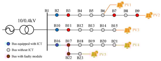
Figure 3.
Topology of the 400 V LVDG test network with 23 buses, showing ICT deployment locations (B2, B10, B16), fault simulation modules (B3, B7, B9, B11, B17, B22), and distributed PV units (yellow symbols at B6, B9, B14, B21, B23).
The system includes three ICTs installed at buses B2, B10, and B16, providing high-precision sampling capabilities with 200 samples per second. The remaining 17 buses (B3–B9, B11–B15, B17–B23) operate without dedicated sampling infrastructure, relying solely on conventional metering electricity meters with 15 min sampling intervals. Five PV units with capacities ranging from 50 to 70 kW are connected at buses B6, B9, B15, B21, and B23, while six buses (B3, B7, B9, B11, B17, B22) are equipped with fault simulation modules to generate various fault scenarios.
The annual operational data, depicted in Figure 4, exhibits significant temporal variations characteristic of LVDG with high PV penetration. The normalized load profile demonstrates typical seasonal patterns with peak demands reaching 0.8 p.u. during summer periods and reduced consumption (0.4–0.6 p.u.) in spring and autumn. PV generation exhibits strong diurnal and seasonal variations, with maximum outputs approaching 0.8 p.u. in summer and winter and minimal generation in spring and autumn. System voltage profiles reveal corresponding fluctuations, with maximum node voltages occasionally exceeding 1.08 p.u. during high PV generation periods and minimum voltages dropping to 0.85 p.u. during peak load conditions.
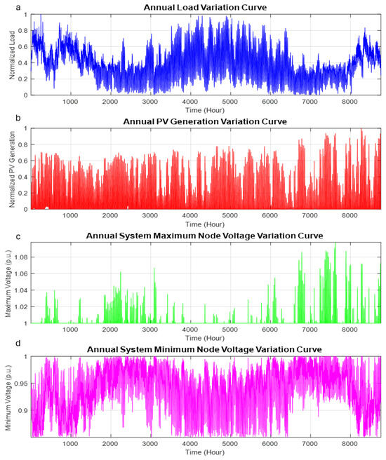
Figure 4.
Annual operational profiles of the test LVDG system: (a) Normalized load variation curve, (b) Normalized PV generation variation curve, (c) Maximum node voltage variation curve, (d) Minimum node voltage variation curve.
To comprehensively evaluate the fault location performance under diverse working conditions, a simulation campaign was conducted using MATLAB/Simulink 2024b. The fault simulation strategy was designed to balance comprehensive coverage with computational efficiency. The simulation generated 600 single-phase-to-ground (AG) fault samples, 300 phase-to-phase (AB) fault samples, 300 three-phase-to-ground (ABCG) fault samples, and 2300 healthy operation samples. Each fault scenario was simulated across six different fault buses (B3, B7, B9, B11, B17, B22), resulting in a total dataset of 9500 samples: (600 + 300 + 300) ∗ 6 + 2300 = 9500.
Finally, the 2D-CNN architecture employed for fault classification and location consists of the following layers, as detailed in Table 3:
Table 3.
2D-CNN Architecture. Input: 80 (time) × W (buses × 3) × 24 (S-transform channels), Each Conv Block includes BatchNorm, ReLU, and Dropout (0.25–0.5).
6.2. Working Condition Clustering Results
The K-means clustering algorithm was applied to the 8760 × 21 feature matrix constructed from annual operational data. The optimal number of clusters was determined to be 6 based on silhouette coefficient analysis, with values ranging from 0.42 to 0.68. Figure 5 illustrates the temporal distribution of the 6 identified working conditions over the year, revealing pronounced seasonal and diurnal patterns.
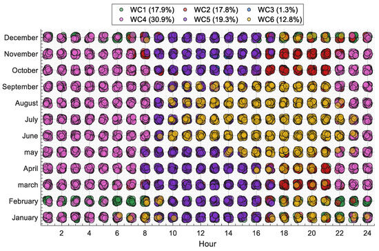
Figure 5.
Temporal distribution of 6 identified working conditions (WC) throughout the year, displayed as a 12 ∗ 24 matrix (months × hours) with color-coded clusters: WC1 (17.9%), WC2 (17.8%), WC3 (1.3%, edge condition), WC4 (30.9%, dominant condition), WC5 (19.3%), and WC6 (12.8%).
As shown in Figure 5, WC4 represents the dominant condition, accounting for 30.9% of the annual duration. It occurs primarily during spring and autumn and is characterized by moderate load and PV generation levels. In contrast, WC3 constitutes an edge condition, representing only 1.3% of the total time and typically corresponding to extreme weather scenarios. The remaining conditions—WC1 (17.9%), WC2 (17.8%), WC5 (19.3%), and WC6 (12.8%)—form a set of regular working conditions reflecting varying levels of PV generation and load demand throughout the year.
To quantitatively characterize these 6 working conditions, Table 3 presents the cluster centroids obtained through K-means algorithm, providing values for representative features selected from the original 21-dimensional feature space. The table includes key operational indicators such as load level (f1), PV output (f8), maximum voltage (f12), minimum voltage (f13), and voltage violation nodes (f17 + f18), along with the corresponding sample counts for each cluster. Figure 6 illustrates the spatial voltage distributions across the 6 identified working conditions (WC1–WC6), derived directly from the cluster centroids presented in Table 4. These distributions reflect characteristic voltage profiles corresponding to distinct generation-load patterns quantified by the centroid features. WC3 exhibits the highest voltage levels (up to 1.05 p.u.), corresponding to high PV injection and light load periods. In contrast, WC6 shows the most pronounced low-voltage levels (down to 0.85 p.u.), indicating high load and low generation conditions. WC4 maintains voltages within a stable and acceptable range (0.95–1.05 p.u.), consistent with the predominant operational states in LVDG.
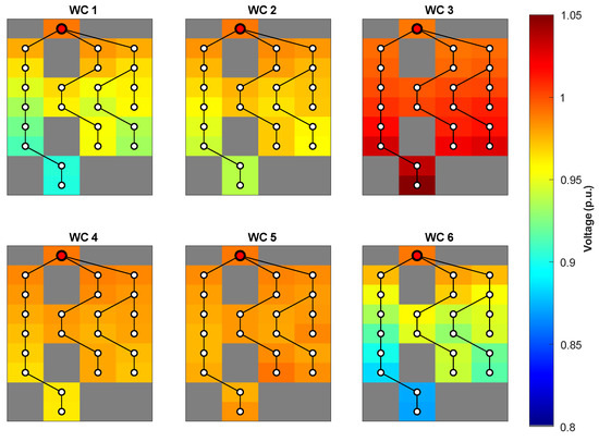
Figure 6.
Spatial voltage distribution heatmaps across the six working conditions in the test network, showing per-unit voltage magnitudes at each bus location. Color gradients from blue (0.8 p.u.) to red (1.05 p.u.) represent voltage levels.
Table 4.
Working Condition Cluster Centroids (Normalized Values).
The voltage variations shown in Figure 6 highlight the operational uncertainty in LVDG resulting from high PV penetration and diverse load profiles, which directly affects the discernibility of fault signatures. As fault-induced changes become increasingly obscured by normal fluctuations under varying conditions, the reliability of conventional fault location methods is significantly challenged. The proposed condition-adaptive method addresses this issue by explicitly accounting for these working disparities, thereby enhancing fault location accuracy across diverse LVDG states. Therefore, training dedicated CNN models tailored to these distinct working conditions enables more precise feature extraction and significantly improves fault location robustness under varying grid operating states.
6.3. S-Transform Enhancement Performance
Fault data were generated in Simulink with measurement units at buses B2, B10, and B16, a 0.02 s sampling interval, and a 2 s analysis window. The dataset comprises 600 A-G, 300 AB, 300 ABC-G, and 2300 normal samples. Each fault type was simulated on six candidate fault lines (B3, B7, B9, B11, B17, B22), yielding 9500 samples in total. All 9500 samples use net-load profiles taken from WC4 in Section 6.2 (the largest operating-condition cluster, 2708 records). Experiments were conducted on a workstation with an Intel i7 CPU, 48 GB RAM, and an RTX 4060 GPU.
The effectiveness of S-transform-based feature extraction is demonstrated through comparative analysis of fault signatures at electrically similar locations. Figure 7 illustrates the challenge of distinguishing faults at buses B17 and B22 when observed from ICT-equipped bus B16. The upper figures show nearly identical voltage amplitude waveforms for A-phase ground faults at both locations, with both signals exhibiting similar transitions from approximately 0.967 p.u. to 0.981 p.u. around the 0.2 s mark, which severely limits the ability of conventional amplitude-based methods to differentiate between these fault points. The middle rows (Figure 7C–F) further indicate that STFT and CWT provide limited separability: STFT concentrates energy near the fundamental with weak time localization, and CWT shows low-contrast, block-like patterns across time-frequency bins. However, the S-transform representations in the lower figures (Figure 7G,H) reveal distinctive time-frequency signatures enabling reliable discrimination. In particular, the S-transform exposes a sharp, time-localized ridge at the event (0.2 s) and systematic differences in the 30–40 Hz band: Sample 5 exhibits noticeably stronger energy across this range, whereas Sample 6 remains much lower. These frequency-domain energy differences, particularly the variations in transient frequency components that are invisible in the time-domain waveforms, provide the discriminative features necessary for accurate fault location identification, thereby supporting the choice of S-transform over amplitude-only, STFT, and CWT-based approaches for feeder-head analysis in LVDGs.
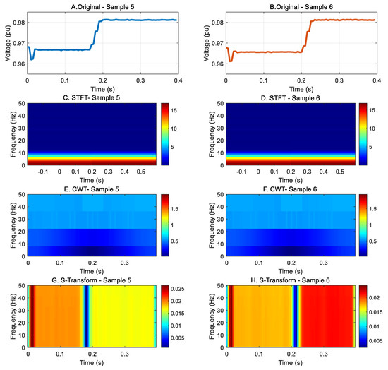
Figure 7.
Comparison of A-phase ground-fault signatures at buses B17 (Sample 5) and B22 (Sample 6) observed from the ICT at bus B16: (A,B) original voltage waveforms, (C,D) STFT time-frequency maps, (E,F) CWT time-frequency maps, (G,H) S-transform time–frequency map.
Figure 8 and Figure 9 present comparative training results for CNN models with and without S-transform preprocessing, respectively. The performance degradation without S-transform enhancement is clearly evident in Figure 8, where fault type classification achieves reasonable accuracy (99.43%), but fault location accuracy plateaus at only 93.17%. The confusion matrix for fault location in Figure 8 reveals significant cross-classification errors between adjacent buses, with substantial off-diagonal elements indicating misclassifications between spatially proximate fault locations. The training curves exhibit slow convergence with persistent oscillations, indicating difficulty in learning discriminative features from raw amplitude data.
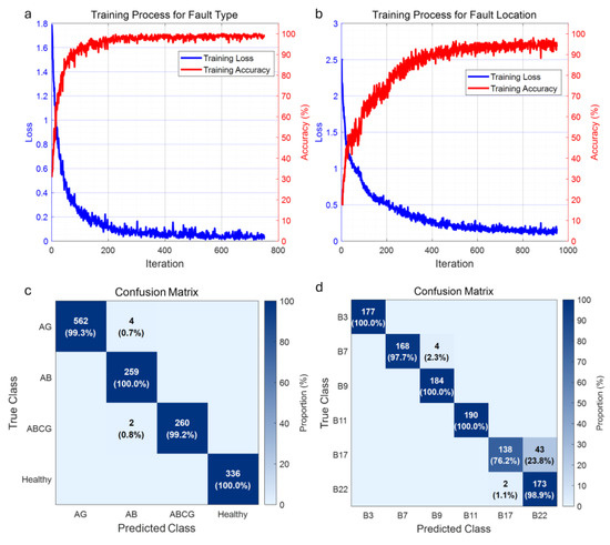
Figure 8.
CNN training performance without S-transform preprocessing: (a) Training curves for fault type classification showing accuracy (red) and loss (blue) evolution; (b) Training curves for fault location showing accuracy (red) and loss (blue) evolution; (c) Confusion matrix for fault type classification; (d) Confusion matrix for fault location.

Figure 9.
CNN training performance with S-transform enhancement: (a) Training curves for fault type classification showing accuracy (red) and loss (blue) evolution; (b) Training curves for fault location showing accuracy (red) and loss (blue) evolution; (c) Confusion matrix for fault type classification; (d) Confusion matrix for fault location.
In contrast, S-transform-enhanced training (Figure 9) demonstrates superior performance across all metrics. Fault type classification reaches 99.72% accuracy, while fault location accuracy achieves 99.80%, representing a substantial 6.63 percentage point improvement. The confusion matrices reveal near-perfect diagonal dominance, with misclassification errors significantly reduced through enhanced spectral-temporal feature discrimination. The accelerated convergence and reduced training loss validate the effectiveness of time-frequency features in capturing fault-specific signatures that remain invisible in conventional amplitude-based analysis.
The quantitative performance comparison is summarized in Table 5 and Table 6. For fault type classification, the S-transform enhancement provides modest improvements of 0.16–0.29% across accuracy, recall, and F1-score metrics. However, for fault location, the S-transform enhancement delivers substantial improvements of 6.63–7.45% across all performance metrics. The fault location accuracy increases from 93.17% to 99.80%, recall improves from 92.46% to 99.81%, and F1-score enhances from 92.37% to 99.82%. This significant performance differential demonstrates that spatial fault discrimination requires fine-grained spectral-temporal analysis that conventional amplitude-based methods cannot provide, particularly under the sparse measurement conditions typical of LVDG deployments.
Table 5.
Performance Comparison for Fault Type Classification With and Without S-Transform Enhancement.
Table 6.
Performance Comparison for Fault Location With and Without S-Transform Enhancement.
In addition, to verify the superiority of the proposed method among comparable approaches, several classical machine-learning models, including SVM, kNN, and random forest, were employed for comparison, and the results are shown in Figure 10. First, in terms of accuracy, the S-transform + CNN method achieves the highest training and testing accuracies of 99.99% and 99.80%, respectively, which are significantly higher than those of the baseline models. Among the traditional approaches, random forest performs best (95.77%/83.12%), followed by SVM (85.12%/82.23%), while kNN shows the lowest accuracy (83.85%/80.25%) due to its limited feature extraction capability. This indicates that conventional time-domain features, such as voltage amplitude alone, are insufficient for precise fault discrimination, whereas combining S-transform time-frequency representations with CNN learning markedly enhances fault-location accuracy and generalization ability. Second, the CNN model requires approximately 180 s for training due to deep network optimization, which is longer than the 2–90 s needed by the baseline models. However, all methods exhibit similar inference times of around 1.3 s. Considering that online operation only requires fast inference, the longer training time does not affect the method’s real-time applicability.
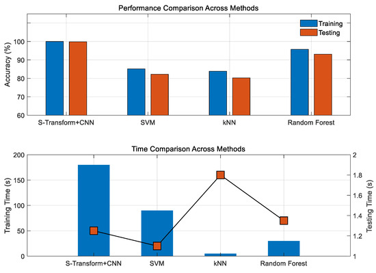
Figure 10.
Comparative performance analysis across different models.
6.4. Transfer Learning Effectiveness
The progressive transfer learning strategy addresses the challenges of sample scarcity and computational efficiency in LVDG fault location under diverse working conditions. This subsection presents a comprehensive evaluation through two distinct experimental scenarios: (i) convergence analysis and accuracy assessment across varying training sample sizes for different working conditions, and (ii) comparative performance evaluation between the proposed condition-adaptive framework and conventional unified approaches.
Figure 11 presents the performance between direct training and the proposed transfer learning strategy across four representative working conditions with varying sample availability. The transfer learning approach, utilizing WC4 (dominant condition) as the source domain, demonstrates superior convergence characteristics across all target domains. For regular conditions (WC1, WC5, WC6), the proposed method achieves 98–99% accuracy with 1000–2000 training samples, representing a 50–60% reduction in data requirements compared to direct training. The performance differential is most pronounced for edge condition WC3, where transfer learning maintains 96% accuracy utilizing merely 100 samples, while direct training saturates at 78% with 350 samples. This 18-percentage-point improvement substantiates the method’s efficacy in mitigating data scarcity challenges.
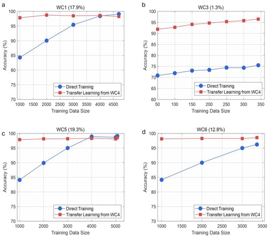
Figure 11.
Performance comparison between direct training and progressive transfer learning across different working conditions with varying training sample sizes. Four representative conditions are evaluated: (a) WC1 (17.9% samples); (b) WC3 (1.3% samples, edge condition); (c) WC5 (19.3% samples); (d) WC6 (12.8% samples).
Figure 12 illustrates the fault location accuracy comparison between unified and condition-adaptive approaches across six working conditions. The unified approach, employing a single CNN trained on the complete dataset without condition differentiation, exhibits significant performance variability with accuracies ranging from 78.5% (WC3) to 98.7% (WC4). This variation indicates the model’s inability to generalize across heterogeneous working conditions, particularly for edge scenarios. Conversely, the proposed condition-adaptive framework, incorporating working condition recognition followed by deployment of condition-specific CNN models, achieves consistent performance with accuracies between 93.2% and 99.8%. The improvement is particularly notable for WC3 (1.3% samples, edge condition) and WC6 (12.8% samples, regular condition), where domain-specific adaptation compensates for distributional shifts. The above results confirm that the integration of working condition clustering with progressive transfer learning effectively addresses both inter-condition heterogeneity and intra-condition data imbalance, ensuring robust fault location performance across the working conditions of LVDG.
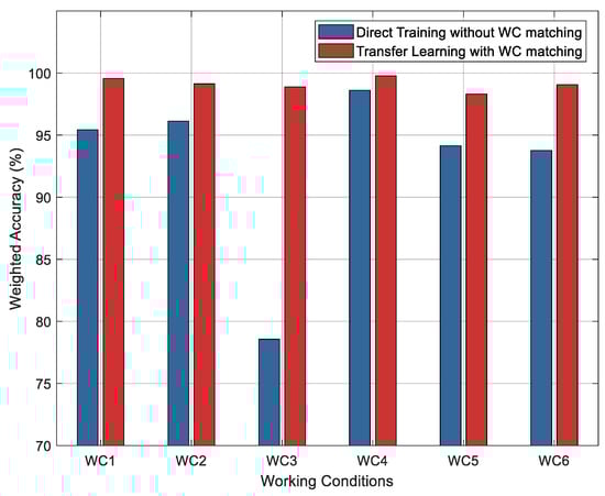
Figure 12.
Comparative analysis of fault location accuracy between direct training without working condition matching (blue bars) and transfer learning with working condition matching (red bars) across six working conditions.
7. Conclusions
This paper has presented an adaptive working condition-based fault location method for low-voltage distribution grids that addresses the dual challenges of limited sampling infrastructure and diverse working conditions introduced by high renewable energy penetration. The proposed method integrates S-transform-enhanced feature extraction with progressive transfer learning to achieve robust fault location performance across heterogeneous grid states.
The key contributions and findings can be summarized as follows:
First, the 21-dimensional working condition clustering model successfully identified 6 distinct operational patterns from year-round LVDG data, with WC4 representing 30.9% of annual operations and WC3 accounting for only 1.3%. This categorization enables targeted model development for scenarios with varying data availability, directly addressing the sample imbalance challenge that has limited conventional ML approaches.
Second, the S-transform enhancement demonstrated substantial improvement in fault discrimination capability under sparse measurement conditions. Comparative analysis revealed that time-frequency features enable differentiation of electrically similar fault locations that produce nearly identical amplitude signatures at feeder head-ends. The method achieved 99.80% fault location accuracy and 99.72% fault type classification accuracy on the 400 V test network, representing improvements of 6.63% and 0.29%, respectively, over conventional amplitude-based approaches.
Third, the progressive transfer learning strategy effectively mitigated data scarcity in edge conditions. By leveraging knowledge from the dominant working condition, the approach maintained 96% accuracy for edge condition WC3 using only 100 training samples, compared to 78% accuracy achieved by direct training with 350 samples. For regular conditions, the method reduced training data requirements by 50–60% while achieving 98–99% accuracy.
Although the current evaluation is simulation-based, our runtime profile indicates that inference with a compact S-transform grid and a lightweight 2D-CNN is compatible with CPU-based edge deployment under sub-second latency while training remains offline, with validation on measured feeder head-end data planned to confirm accuracy and latency in practice. Additionally, we note the risk of negative transfer when source and target conditions differ (e.g., ICT-induced signal drift, topology updates, or scarce/noisy labels), and future work will quantify it, add simple pre-transfer guards, define recovery rules, and test robustness to drift and data scarcity/noise.
Author Contributions
Conceptualization, L.X., D.X. and F.X.; methodology, F.X. and Z.W.; software, Y.Z. and Z.Q.; validation, J.Z. and Z.Q.; writing—original draft preparation, F.X.; writing—review and editing, H.L. and L.X. All authors have read and agreed to the published version of the manuscript.
Funding
This research was funded by State Grid Zhejiang Electric Power Co., Ltd. Quzhou Power Supply Company under project no. SGZJQZ00KGWT2500660 for the project “Digital Twin-Based Low-Voltage Fault Location and Frequent Outage Mitigation Technology”.
Data Availability Statement
The original contributions presented in this study are included in the article. Further inquiries can be directed to the corresponding author.
Conflicts of Interest
Author Fengqian Xu, Zhenyu Wu, Yong Zheng, and Jianfeng Zheng were employed by the State Grid Quzhou Power Supply Company. The remaining authors declare that the research was conducted in the absence of any commercial or financial relationships that could be construed as a potential conflict of interest.
Abbreviations
The following abbreviations are used in this manuscript:
| LVDG | Low-voltage distribution grid |
| CNN | Convolutional neural network |
| RES | Renewable energy sources |
| PV | Photovoltaic |
| ML | Machine learning |
| k-NN | K-nearest neighbors |
| SVM | Support vector machines |
| ICT | Integrated smart terminal |
| WC | Working condition |
References
- Hache, E.; Palle, A. Renewable energy source integration into power networks, research trends and policy implications: A bibliometric and research actors survey analysis. Energy Policy 2019, 124, 23–35. [Google Scholar] [CrossRef]
- Kotsonias, A.; Hadjidemetriou, L.; Asprou, M.; Kyriakides, E. Operational challenges and solution approaches for low voltage distribution grids—A review. Electr. Power Syst. Res. 2025, 239, 111258. [Google Scholar] [CrossRef]
- Mora-Florez, J.; Meléndez, J.; Carrillo-Caicedo, G. Comparison of impedance based fault location methods for power distribution systems. Electr. Power Syst. Res. 2008, 78, 657–666. [Google Scholar] [CrossRef]
- Naidu, O.D.; Pradhan, A.K. A traveling wave-based fault location method using unsynchronized current measurements. IEEE Trans. Power Deliv. 2018, 34, 505–513. [Google Scholar] [CrossRef]
- Khoa, N.M.; Cuong, M.V.; Cuong, H.Q.; Hieu, N.T.T. Performance comparison of impedance-based fault location methods for transmission line. Int. J. Electr. Electron. Eng. Telecommun. 2022, 11, 234–241. [Google Scholar] [CrossRef]
- Sayal, A.; Kumar, S.; Singh, P.; Verma, A. Neural Networks And Machine Learning. In Proceedings of the 2023 IEEE 5th International Conference on Cybernetics, Cognition and Machine Learning Applications (ICCCMLA), Hamburg, Germany; 2023; pp. 58–63. [Google Scholar] [CrossRef]
- Chuan, O.W.; Ab Aziz, N.F.; Yasin, Z.M.; Salim, N.A.; Wahab, N.A. Fault classification in smart distribution network using support vector machine. Indones. J. Electr. Eng. Comput. Sci. 2020, 18, 1148–1155. [Google Scholar] [CrossRef]
- Okumus, H.; Nuroglu, F.M. A random forest-based approach for fault location detection in distribution systems. Electr. Eng. 2021, 103, 257–264. [Google Scholar] [CrossRef]
- Gangwar, A.K.; Shaik, A.G. k-Nearest neighbour based approach for the protection of distribution network with renewable energy integration. Electr. Power Syst. Res. 2023, 220, 109301. [Google Scholar] [CrossRef]
- Rizeakos, V.; Bachoumis, A.; Andriopoulos, N.; Dikaiakos, C.; Vita, V.; Pavlatos, C. Deep learning-based application for fault location identification and type classification in active distribution grids. Appl. Energy 2023, 338, 120932. [Google Scholar] [CrossRef]
- Siddique, M.N.I.; Shafiullah, M.; Mekhilef, S.; Pota, H.; Abido, M.A. Fault classification and location of a PMU-equipped active distribution network using deep convolution neural network (CNN). Electr. Power Syst. Res. 2024, 229, 110178. [Google Scholar] [CrossRef]
- Rusyn, B.; Lutsyk, O.; Kosarevych, R.; Kynash, Y.; Lozynskyi, A. Rethinking Deep CNN Training: A Novel Approach for Quality-Aware Dataset Optimization. IEEE Access. 2024, 12, 137427–137438. [Google Scholar] [CrossRef]
- Fan, F.J.; Shi, Y. Effects of data quality and quantity on deep learning for protein-ligand binding affinity prediction. Med. Chem. 2022, 72, 117003. [Google Scholar] [CrossRef]
- Mirshekali, H.; Dashti, R.; Keshavarz, A.; Shaker, H.R. Machine learning-based fault location for smart distribution networks equipped with micro-PMU. Sensors 2022, 22, 945. [Google Scholar] [CrossRef]
- Trindade, F.C.; Freitas, W. Low Voltage Zones to Support Fault Location in Distribution Systems With Smart Meters. IEEE Trans. Smart Grid 2017, 8, 2765–2774. [Google Scholar] [CrossRef]
- Biswas, R.S.; Azimian, B.; Pal, A. A Micro-PMU Placement Scheme for Distribution Systems Considering Practical Constraints. In Proceedings of the 2020 IEEE Power & Energy Society General Meeting (PESGM), Montreal, QC, Canada, 2–6 August 2020; pp. 1–5. [Google Scholar] [CrossRef]
- Mohassel, R.R.; Fung, A.; Mohammadi, F.; Raahemifar, K. A Survey on Advanced Metering Infrastructure. Int. J. Electr. Power Energy Syst. 2014, 63, 473–484. [Google Scholar] [CrossRef]
- Duan, N.; Huang, C.; Sun, C.C.; Min, L. Smart meters enabling voltage monitoring and control: The last-mile voltage stability issue. IEEE Trans. Ind. Inform. 2021, 18, 677–687. [Google Scholar] [CrossRef]
- Qiu, H.; Zhang, J.; Zhou, J.; Shi, G.; Yao, G.; Cai, X. A novel delta-type transformer-less unified power flow controller with multiple power regulation ports. IEEE Trans. Power Electron. 2025, 40, 15820–15834. [Google Scholar] [CrossRef]
- Xu, X.; Deng, J.; Lin, H.; Li, Z.; Wen, H. Lightweight anomalous detection of hydro turbine operation sound using fusion network enhanced by load information. IEEE Trans. Instrum. 2025, 74, 1–13. [Google Scholar] [CrossRef]
- Hossain, J.; Pota, H.R. Robust Control for Grid Voltage Stability: High Penetration of Renewable Energy; Power systems; Springer: Singapore, 2014; pp. 123–126. [Google Scholar]
- Hacıoğlu, V. Observability and Learnability as Opposed to ‘Seen and Unseen’; Palgrave Macmillan: Cham, Switzerland, 2024; pp. 143–168. [Google Scholar] [CrossRef]
- Wang, X.; Wang, H.; Peng, M. Interpretability study of a typical fault diagnosis model for nuclear power plant primary circuit based on a graph neural network. Reliab. Eng. Syst. Saf. 2025, 261, 111151. [Google Scholar] [CrossRef]
- Wang, J.; Song, Y.; He, T. A novel adaptive monitoring framework for detecting the abnormal states of aero-engines with maneuvering flight data. Reliab. Eng. Syst. Saf. 2025, 258, 110910. [Google Scholar] [CrossRef]
- Saldaña-González, A.E.; Aragüés-Peñalba, M.; Sumper, A. Distribution network planning method: Integration of a recurrent neural network model for the prediction of scenarios. Electr. Power Syst. Res. 2024, 229, 110125. [Google Scholar] [CrossRef]
- Wang, Y.; Cui, Q.; Weng, Y.; Li, D.; Li, W. Learning picturized and time-series data for fault location with renewable energy sources. Int. J. Electr. Power Energy Syst. 2023, 147, 108853. [Google Scholar] [CrossRef]
- Liu, G.; Liu, J.; Bai, Y.; Wang, C.; Wang, H.; Zhao, H.; Liang, G.; Zhao, J.; Qiu, J. Eweld: A large-scale industrial and commercial load dataset in extreme weather events. Sci. Data 2023, 10, 615. [Google Scholar] [CrossRef]
- Gonçalves, A.C.; Costoya, X.; Nieto, R.; Gimeno, L.; Gámiz-Fortis, S.R. Extreme weather events on energy systems: A comprehensive review on impacts, mitigation, and adaptation measures. Sustain. Energy Res. 2024, 11, 4. [Google Scholar] [CrossRef]
- Xu, L.; Chow, M.Y.; Taylor, L.S. Power Distribution Fault Cause Identification With Imbalanced Data Using the Data Mining-Based Fuzzy Classification E-Algorithm. IEEE Trans. Power Syst. 2007, 22, 164–171. [Google Scholar] [CrossRef]
- Ma, R.; Eftekharnejad, S.; Zhong, C.; Gursoy, M.C. A Predictive Online Transient Stability Assessment With Hierarchical Generative Adversarial Networks. IEEE Trans. Power Syst. 2022, 37, 4762–4773. [Google Scholar] [CrossRef]
- Mukherjee, D.; Chakraborty, S.; Banerjee, R. Power system fault classification with imbalanced learning for distribution systems. In Proceedings of the 2020 IEEE 7th Uttar Pradesh Section International Conference on Electrical, Electronics and Computer Engineering (UPCON), Prayagraj, India, 27–29 November 2020; pp. 1–6. [Google Scholar] [CrossRef]
Disclaimer/Publisher’s Note: The statements, opinions and data contained in all publications are solely those of the individual author(s) and contributor(s) and not of MDPI and/or the editor(s). MDPI and/or the editor(s) disclaim responsibility for any injury to people or property resulting from any ideas, methods, instructions or products referred to in the content. |
© 2025 by the authors. Licensee MDPI, Basel, Switzerland. This article is an open access article distributed under the terms and conditions of the Creative Commons Attribution (CC BY) license (https://creativecommons.org/licenses/by/4.0/).