Article

Multi-Objective Optimization of Sucker Rod Pump Operating Parameters for Efficiency and Pump Life Improvement Based on Random Forest and CMA-ES

1
School of Petroleum and Natural Gas Engineering, Changzhou University, Changzhou 213164, China
2
School of Mechanical Engineering, Changzhou Institute of Technology, Changzhou 213032, China
*
Author to whom correspondence should be addressed.
Processes 2025, 13(12), 3871; https://doi.org/10.3390/pr13123871 (registering DOI)
Submission received: 2 November 2025 / Revised: 24 November 2025 / Accepted: 26 November 2025 / Published: 1 December 2025

Abstract

The design parameters of the sucker rod pumping unit (SRPU) are influenced by multiple factors. Traditional methods based on oil production engineering theories involve numerous simplifications, making it difficult to effectively address the complex realities of oilfields, thereby requiring improvement in the reliability of pumping system design solutions. This paper, based on the massive design schemes and corresponding operational performance data accumulated during the long-term development of oilfields, innovatively proposes an intelligent optimization model combining Random Forest and Covariance Matrix Adaptation Evolution Strategy algorithm (CMA-ES). This model overcomes the shortcomings of insufficient data and incomplete design indicators in the establishment of lifting design models. By standardizing and processing the data from 5000 historical lifting scheme sets, a sample database of SRPU lifting system designs was created, covering dimensions such as well geology, fluid, and production. Based on this, aiming at system efficiency and pump life expectancy, geological development characteristic parameters and lifting design parameters were taken as variables to establish a predictive model for the operation effect of the lifting system. The dataset was divided into 8:1:1 subsets for training, hyperparameter tuning and performance testing. Subsequently, an optimization model was established to jointly optimize the lifting system design parameters. Case studies show that the intelligent optimization method can simultaneously optimize parameters such as pump setting depth, pump diameter, stroke, and frequency, with expected improvements in system efficiency of 6.75% and pump life expectancy of 29%.

1. Introduction

The sucker rod pumping unit (SRPU) is a widely used artificial lifting method [1], rational design of SRPU can improve the production performance and efficiency of the wells, extend the pump life expectancy, and is an important direction to improve oilfield efficiency [2]. Flow-assurance issues such as asphaltene deposition can affect well productivity and the stable operation of lifting systems [3]. Recent studies have shown that injection pressure and flow rate are closely tied to equipment performance, and improving petroleum engineering machinery therefore has a direct impact on reservoir stimulation and long-term recovery efficiency [4,5]. Due to the many factors that need to be considered in the optimization process, such as geological conditions, production requirements, and economic factors, optimizing the design of SRPU is a highly challenging task.
Current SRPU design research broadly follows two streams. Physics- and simulation-based approaches use production-engineering theory and system models to approximate field conditions and screen candidate configurations, but they rely on simplifying assumptions and often require manual comparison of a limited set of designs, which can miss globally competitive solutions. Data-driven approaches learn from historical designs and pair predictors with optimization to balance production and energy use; however, their effectiveness depends on data scale and coverage, completeness of the factor set and objectives, and careful model selection to capture complex multi-factor interactions. These observations motivate our prediction-optimization framework for SRPU design.
Previous research primarily focuses on the impact of SRPU parameters or operating conditions on system efficiency, energy consumption, and production. On one hand, there is a problem of insufficient data, as only a few hundred data points have been used to optimize the model of the beam pumping units. Additionally, there is an issue of incomplete design objectives, as only SRPU parameters or operating conditions are used to construct predictive optimization models for efficiency, energy consumption, and production, which affects the accuracy and effectiveness of the optimization results. On the other hand, data-driven optimization methods typically require the construction of complex models to describe the operational patterns of the pump jack system, ensuring good performance on training data. Most previous studies have used neural networks to build predictive models, but further exploration is needed to determine which model can achieve better fitting and prediction results.
To enhance the reliability and accuracy of lifting schemes, a data-driven approach should be applied to explore patterns in historical lifting system design solutions of pumping units, combining the characteristics of pumping unit lifting system design variables with geological development parameters, establishing a lifting system design effect prediction model with lifting design operation as the target. By predicting the lifting operation effects accurately based on different combinations of lifting design parameters, a further optimization mathematical model of the lifting system design is established, calling upon the effect prediction model with the goal of optimizing operational effects. The lifting system design parameters are iteratively optimized to obtain the best design solution.
This paper makes the following major contributions.
A unified SRPU design prediction-optimization framework is developed, which integrates the rapid predictive capability of the Random Forest regression model with the global search efficiency of the CMA-ES algorithm. Through this integrated approach, efficient exploration of the high-dimensional lift-parameter design space is enabled under specified operational constraints.
A high-quality dataset of 5000 historical lifting cases was constructed, and 15 key indicators were extracted through feature-importance analysis and multicollinearity filtering, thereby establishing a reliable data foundation for performance prediction.
The rest of the paper is organized as follows. In Section 2, offers a systematic literature review coupled with a comparative analysis of related work. In Section 3, a mathematical model for optimizing the design of lifting systems is established. In Section 4, a predictive model for lifting system performance based on the Random Forest algorithm is constructed. Section 5 presents an intelligent optimization model for lifting design parameters based on the CMA-ES algorithm. Section 6 two test cases are examined. Section 7 summarizes the main conclusions.

2. Related Work

2.1. Physics and Simulation-Based Approaches

Hansen et al. proposed a model predictive controller that maintains fluid level by adjusting rod-pump plunger speed while optimizing a coupled rod–well–reservoir model to represent dynamic well conditions [6]. Xing et al. developed a nonlinear friction simulation for the pumping rod string and analyzed friction sensitivity factors to guide rod-pumping system design [7]. Lv et al. introduced an Equivalent Vibration Model (EVM) for continuous SRPU systems to rapidly predict plunger displacement and polished-rod load, supporting efficient design studies [8]. He established a 3-D mechanical model for inclined-shaft pumping pumps and an optimization model for anti-deviation grinding structure and safe position, optimizing combinations of well pipes using actual field data [9]. Langbauer et al. proposed a software-based frequency-elastic drive mode employing power-frequency feedback control, with its load- and energy-reduction effects validated by full-system simulations and field tests [10]. Jalikop et al. validated Computational Fluid Dynamics (CFD) model of internal SRPU flow explains mid-cycle standing-valve closure and predicts a square-root scaling of the critical plunger speed with the ball–fluid density ratio [11].
While more comprehensive than closed-form formulas, these methods can be complex and still depend on idealizations; in practice, engineers often construct and compare a small number of simulated designs, which does not guarantee the true optimum.

2.2. Data-Driven Prediction and Intelligent Optimization

Gu et al. trained neural networks on 3000 training and 324 test samples to predict stroke, load extrema, pump efficiency, production, and power, and then used a strength-Pareto evolutionary algorithm to maximize oil production while minimizing power consumption [12]. Han et al. formulated a mathematical model for casing gas-assisted rod pumping and applied genetic algorithms and particle swarm optimization to tune gas pressure, liquid viscosity, and rod length, improving efficiency and reducing energy consumption [13]. Shi et al. selected 11 parameters (e.g., fluid properties, liquid production capacity, well trajectory, pump depth) to build a comprehensive evaluation function over pump efficiency, tons of liquid consumption per hundred meters, and annual operating and maintenance costs, and trained a deep recursive neural network to select the best artificial-lift method [14]. Feng et al. used 500 training and 100 test sets with SRPU structural parameters and operating conditions as inputs to build a neural predictive-optimization model correlating pump-model parameters with system efficiency, targeting SRPU model optimization [15].
Overall, the success of data-driven SRPU design hinges on data adequacy, factor/objective completeness, and appropriate model choice to reflect complex interactions, key determinants for achieving genuine intelligent automation in lifting-system design [16].

3. Mathematical Model of Lifting System Design

Optimization of the design parameters for the lifting system is based on the geological, fluid, and production indicators of the oil well. The goal is to find the optimal lifting design parameters, including stroke, frequency, pump setting depth, pump diameter, while meeting the production requirements of the well. This optimization aims to ensure that the lifting system operates to meet production demands, improve operational efficiency, and extend the life of the oil well [17].
From a mathematical perspective, the optimization of design parameters for the lifting system falls into the category of multi-objective constrained nonlinear mixed-integer programming problems (CMINP). The objective of CMINP is to find the optimal solution for a set of decision variables while satisfying a set of constraints, such that multiple objective functions are optimized or approximated to their optimum [18,19]. When optimizing the design parameters of the lifting system, it is necessary to first determine the objective function, optimization variables, and constraints.

3.1. Optimization Variables

Optimization variables refer to the parameters that need to be optimized or designed in an optimization problem. These parameters can vary independently within a certain range. For the optimization problem of pump jack lifting system design parameters, the optimization variables include stroke, frequency, pump setting depth, pump diameter. Among these, stroke (H), stroke frequency (F), and pump setting depth (B) are continuous variables, while pump diameter (P) is a discrete variable. Different combinations of these parameters correspond to different design solutions.

3.2. Objective Function

The objective function, which is the mathematical expression of performance indicators, is used to evaluate the quality of a design solution. For the optimization of the lifting system design of the pump well, the system efficiency and the pump life expectancy are selected as objective functions. System efficiency refers to the ratio of the energy input at the surface converted by the pump well lifting system to the required energy for liquid uplift, reflecting the energy utilization efficiency of the pump well lifting system [20,21]. Improving system efficiency can reduce energy consumption, save costs, and reduce environmental pollution [22]. The pump life expectancy refers to the time interval between one pump inspection operation and the next in a pump well, reflecting the operational stability and reliability of the pump well lifting system [23]. Extending the pump life expectancy can reduce downtime, lower maintenance costs, and increase production efficiency [24].
The selected function variables include four lifting design parameters: stroke, frequency, pump setting depth, pump diameter, as well as geological development characteristic parameters such as dynamic liquid level, water cut, and daily liquid production capacity, among others.
The stroke is the distance between the traveling barrel of the pump jack when it moves between the top limit position and bottom limit position during operation; the frequency is the number of up-and-down reciprocating movements of the pumping rod per minute in the pump well; pump setting depth refers to the distance from the pump’s base plate down to the pump’s suction port. Pump diameter refers to the outer diameter of the working barrel of the pump in a deep well. The expression of the objective function is as follows:
max S   ( H , F , B , P , M )
max T   ( H , F , B , P , M )
M = M 1 , M 2 , , M n
where H represents the stroke, F represents the frequency, B represents the pump setting depth, P represents the pump diameter, geological development feature M has n indicators, S (H, F, B, P, M) is the function of system efficiency, and T (H, F, B, P, M) is the function of pump life expectancy.

3.3. Constraints

The constraint conditions refer to a series of limitations on the values of the optimization variables. The closer these constraint conditions are to actual production conditions, the closer the solution space and the final solution will be to practical production. For the optimization problem of the lifting system design of the pump well, the following possible constraint conditions are introduced:
(1) Upper and lower limit constraints on the stroke (H), frequency (F), and pump setting depth (B) are determined based on the range of lifting system design indicators in the database, establishing limits on the range of stroke, frequency, and pump setting depth.
H H min , H max
F F min , F max
B B min , B max
where Hmin represents the minimum stroke value, Hmax represents the maximum stroke value, Fmin represents the minimum frequency value, Fmax represents the maximum frequency value, Bmin represents the minimum pump setting depth value, and Bmax represents the maximum pump setting depth value.
(2) Upper and lower limit constraints on the pump diameter (P) refer to the outer diameter of the working barrel of the pump in a deep well, restricting the range of pump diameters for each well within given limits.
P P 1 , P 2 , , P n
where Pn represents the pump diameter value.
(3) Upper and lower limit constraints on submergence depth (G) refer to the depth below the dynamic liquid level at which the pump is submerged, calculated as the difference between pump depth (B) and dynamic liquid level (D), where G = BD. Therefore, submergence depth varies with changes in pump depth. It is important to keep the submergence depth within a reasonable range, neither too large nor too small.
G G min , G max
where Gmin represents the minimum submergence depth value, and Gmax represents the maximum submergence depth value
(4) Displacement constraint: The product of stroke, frequency, and pump diameter needs to remain approximately constant, denoted as C. In the optimization process, two variables are selected as decision variables, and the third is computed from them. When the computed value exceeds its allowable range, a penalty term is added to the objective function.
H × F × P = C
Reasonable upper and lower bounds help the optimization run more efficiently. In this study, these limits are drawn from the data range or set by field engineers according to practical experience.

4. Lifting System Performance Prediction Model

There are different calculation methods for the objective function. The traditional design method of the oil pumping system, based on petroleum engineering theory, predicts the performance indicators of the lifting system, often using assumed values and simplified equivalent models, which are subjective and result in less than ideal on-site operational results. Similar issues appear in hydrate-risk prediction models for deep-water wells [25]. Therefore, a data-driven lifting design method has been developed, which constructs an intelligent prediction model based on a large amount of historical data to achieve performance prediction under different lifting system design parameters.

4.1. Establishment of the Sample Library

Data related to the lifting system design of 5000 oil pumping wells in a certain oilfield was collected, covering indicators from dimensions such as geological characteristics, fluids, and production. The dataset used in this study is from an oilfield in eastern China, with wells distributed across integrated, fault-block, low-permeability, and heavy-oil reservoirs. These reservoir types ensure that the lifting-system design indicators cover a wide range of operating conditions. Combining petroleum engineering theory and expert experience, a set of indicators for the lifting system design was further determined, including 17 geological development characteristic indicators such as dynamic liquid level, water cut, daily liquid production capacity, and crude oil density; 4 lifting system design indicators such as stroke, frequency, pump setting depth, and pump diameter; and 2 operational performance indicators such as system efficiency and pump life expectancy.
To enhance the reliability of the data, data cleansing was performed on the indicators. Missing data were supplemented through interpolation. Data anomalies were monitored using the 3σ principle, and experts cross-checked and corrected the data based on their understanding.
To improve sample quality and reduce data processing dimensions, the Mean Decrease Impurity (MDI) method was used to analyze the main influencing factors of the lifting indicators. MDI is a feature selection method based on Random Forest, where the reduction in prediction error after adding a feature is used as the evaluation criterion for feature importance [26]. The importance of each feature was calculated in turn, and the features were ranked according to their importance, as shown in Figure 1.
A cumulative contribution of 0.95 is widely accepted as the cutoff, and this threshold is applied in determining the selected features.
From Figure 1, it can be seen that when the feature importance threshold is set to 0.03, removing six low-variance indicators including casing pressure, annual water production, back pressure, crude oil density, monthly gas production, and annual oil production, the sum of the remaining 15 indicators is 0.946.
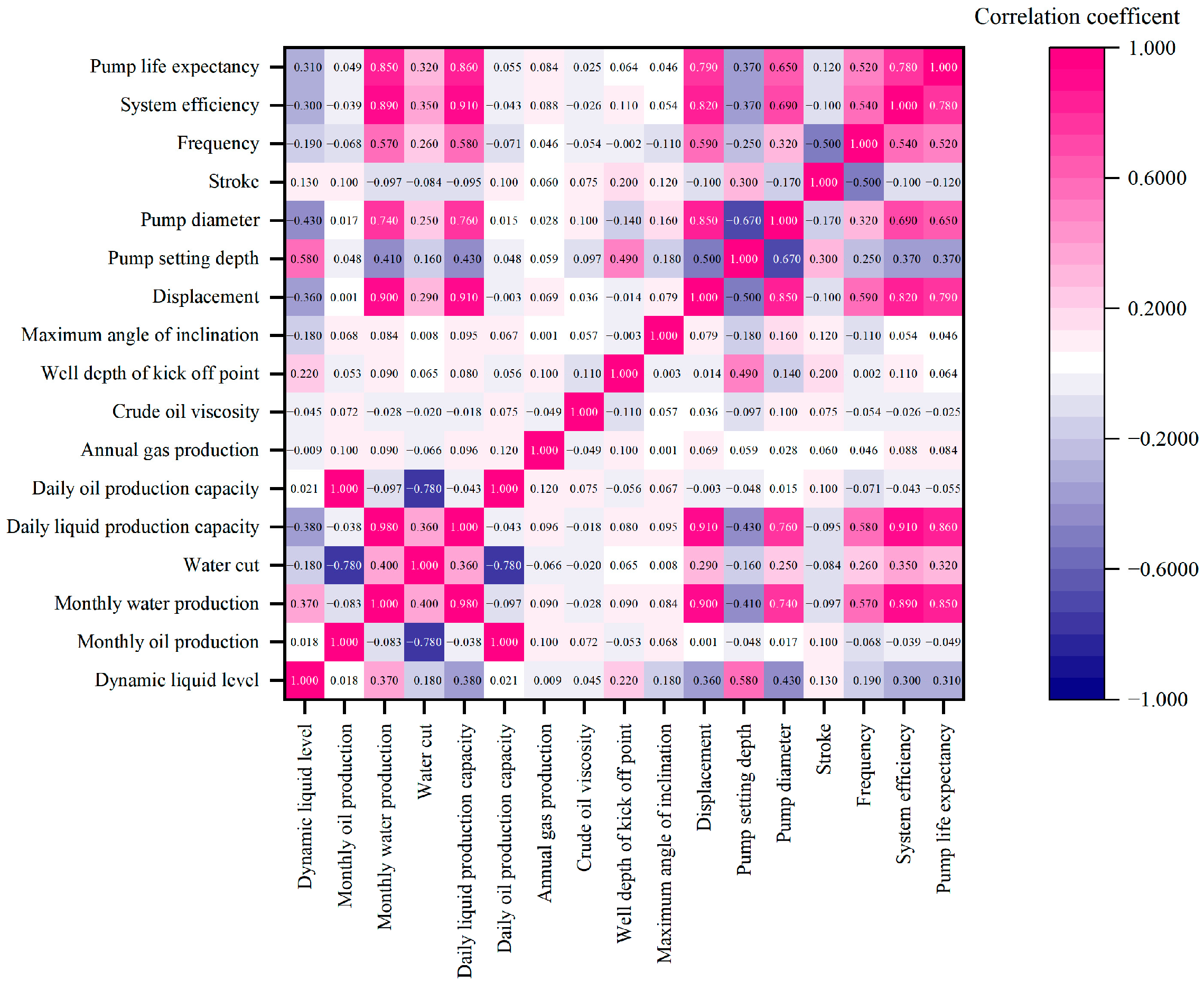
Based on this, the remaining 15 indicators were analyzed for multicollinearity using pairwise Pearson correlations [27,28]. Indicators with high correlation (greater than 0.8) were considered redundant. This threshold was selected because correlation coefficients between 0.8 and 1.0 are categorized as “very strong,” whereas 0.6–0.8 are considered “moderately strong” according to established guidelines [29]. The correlation analysis is shown in Figure 2.
Comparing all features pairwise, if the absolute value of the Pearson correlation coefficient between two features exceeds the threshold of 0.8, then one of the features is removed. From Figure 2, it can be observed that the Pearson correlation coefficient between monthly water production and daily liquid capacity is 0.98, the displacement and daily liquid capacity have a correlation coefficient of 0.91, and the displacement and monthly water production are correlated with a coefficient of 0.9, displacement and pump diameter are correlated with a coefficient of 0.85. Therefore, two highly correlated indicators, including monthly water production, and displacement, were removed.
After the above processing, a sample library for the lifting system design of 5000 oil pumping wells was prepared. It includes a total of 15 lifting system design indicators: 9 geological development characteristic indicators such as dynamic liquid level, monthly oil production, water cut, daily oil production capacity, daily liquid production capacity, annual gas production, crude oil viscosity, depth of kick off point, and maximum well inclination angle; 4 lifting system design parameter indicators such as stroke, frequency, pump setting depth, and pump diameter; and 2 operational performance indicators such as system efficiency and pump life expectancy.
All historical field data used in this study were checked on site to ensure their validity. Although field measurements inevitably contain some uncertainty, the large dataset and the robustness of the Random Forest model help reduce the impact of individual noisy samples.

4.2. Model Architecture

In order to build an effect prediction model for the lifting system design, the Random Forest algorithm is used as the predictive model, Random Forest is a machine learning algorithm that uses decision trees as learners and introduces random attribute selection based on decision trees [30]. For the established model, based on input geological development characteristic data and lifting system design parameters, the operational performance of the lifting system design scheme can be obtained, reflecting clearly the strengths and weaknesses of the design [31]. The process of constructing the Random Forest in this algorithm is as follows:
(1) The constructed sample set is divided into three categories of training set A, validation set B, and test set C in an 8:1:1 ratio. The training set data are used to train the model and determine the hypothesis function parameters; the validation set data are used to optimize the model hyperparameters, select the best-performing hyperparameter combination, and determine the optimal model; the test set data are used to evaluate the model’s performance. T times of bootstrapping are conducted from training set A to form T sampling sets;
(2) A Random Forest model consisting of T regression trees is built for each of the T sampling sets, and the node parameters of each model can be optimized using grid search methods [32]. The final prediction result is the average of the regression results of each decision tree model;
(3) The hyperparameters of the model are adjusted on the validation set to monitor whether the model is overfitting and to conduct an initial evaluation of the prediction model;
(4) The difference between the model’s prediction results and the actual numerical simulation results on the test set is compared to evaluate the prediction effectiveness of the model.

4.3. Training Method and Performance Evaluation

The coefficient of determination (R2), a commonly used metric in machine learning, is chosen to evaluate the performance of a random forest on the training, validation, and test sets [33]. The R2 value reflects how well the estimated values from the trend line fit the actual data. The closer the R2 value is to 1, the higher the degree of fit, and the more reliable the trend line is. The formula for R2 is as follows:
R 2 = SSR SST = i = 1 n ( y i ^ y i ¯ ) 2 i = 1 n ( y i y i ¯ ) 2
where SSR represents the sum of squared differences between the predicted values and the mean of the original values, while SST represents the sum of squared differences between the original data and its mean. Here, y i ^ denotes the predicted data, y i ¯ denotes the mean of the original data, and y i represents the original data.

5. Design of the Intelligent Optimization Algorithm

When designing the lifting system for pumping units, different design schemes are often considered simultaneously. The optimal design strategy varies under different geological development conditions. In the actual development and adjustment of oilfield schemes, it is often necessary to adjust the lifting system design and related systems simultaneously. At this point, the mutual influence of the schemes needs to be fully considered, and simultaneous optimization of stroke, frequency, pump setting depth, pump diameter is required. The combination optimization problem is more complex than single-parameter optimization problems, as it involves more optimization variables and a more complex mathematical model.

5.1. CMA-ES Algorithm

For the optimization of the lifting system design scheme, the original geological parameters of the target well and the design parameters of the lifting system are input into the established intelligent prediction model. Based on the prediction results, intelligent optimization algorithms are used to continuously update and adjust the indicator parameters, further optimizing the lifting system design scheme to achieve the best predicted results. The Covariance Matrix Adaptation Evolution Strategy algorithm (CMA-ES) is employed to optimize the design parameters of the lifting system. CMA-ES algorithm belongs to the class of evolutionary strategy algorithms and is mainly used to solve complex nonlinear and non-continuous optimization problems [34]. It can be applied in various fields such as global optimization, multimodal optimization, multi-objective optimization, and large-scale optimization [35]. By analyzing the principles of the CMA-ES algorithm and considering the characteristics of the pumping unit well lifting system design, the intelligent optimization algorithm needs to address the following challenges.

5.2. Target Conversion

The study selects two indicators, system efficiency and pump life expectancy, as the optimization objectives for the lifting system [36,37]. Therefore, it is necessary to first transform the multi-objective problem into a single-objective problem. Furthermore, due to the different dimensions and orders of magnitude of system efficiency and pump life expectancy, in order to reduce the significant differences between the evaluation indicators and ensure the reliability of the results, the study uses the linear weighted sum method to assign appropriate weight coefficients to system efficiency and pump life expectancy according to their importance. The product sum is then used as the new objective function as follows.
max S T = S   ( H , F , B , P , M ) × K + T   ( H , F , B , P , M ) × ( 1 K )
where K represents the weight coefficient of the objective function. By adjusting the value of K based on the numerical values of system efficiency and pump life expectancy for different lifting design methods, the optimization solution can be improved to meet the expectations of decision-makers.
Equation (11) applies a linear weighted-sum to combine system efficiency and pump life into a single objective. This method is simple to use but sensitive to weight scaling, and it only explores the convex part of the Pareto set. Consequently, it provides one compromise solution rather than a full Pareto front. More complete multi-objective methods (e.g., NSGA-II or the ε-constraint method) could capture the full trade-off, but at a higher computational cost.

5.3. Transform Discrete Data into Continuous

The CMA-ES is primarily used to solve continuous optimization problems. In the lifting system design parameters, variables such as stroke, frequency, and pump setting depth are continuous, while pump diameter is a discrete data type. To handle the discrete variable of pump diameter, a small continuous interval is used to represent an integer value. However, when evaluating the objective function and constraints, it will be converted back to the corresponding integer value. This method can be described as follows [38].
The possible values of the pump diameter P belong to a discrete set, p = p 1 , p 2 , , p n . Define a position variable k, represented as:
k = r o u n d ( x ) , x 1 , n
where n is the size of the set p, x is a continuous variable of 1 to n, and round is used to convert x into an integer value, the corresponding integer variable:
P = p ( k ) = p k

5.4. Processing Strategy for Nonlinear Constraints

The penalty function method is the most commonly used approach for handling constraints. Its basic idea is to add a penalty term when calculating the objective function value for individuals that do not satisfy the constraints, making their objective function fitness worse so that they naturally get eliminated during the function optimization process [36]. In the specific implementation process, a penalty term Q (H, F, B, P, M) is added to the objective function ST (H, F, B, P, M) to construct a penalty fitness function eval (H, F, B, P, M):
S T e v a l = S T   ( H , F , B , P , M ) + Q   ( H , F , B , P , M )
where the penalty term Q (H, F, B, P, M) is the penalty for a solution that does not satisfy the constraint.
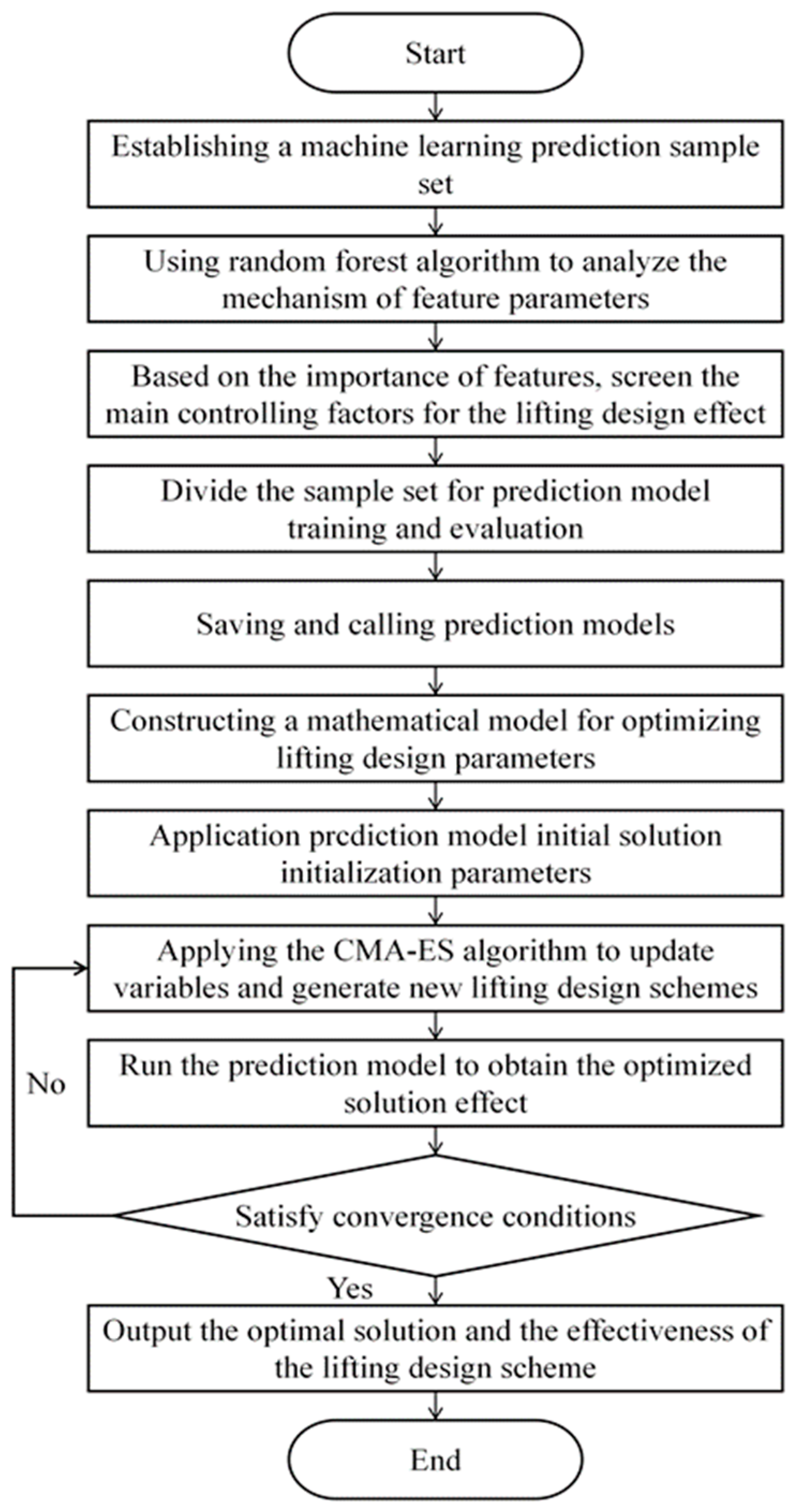
On this basis, the overall intelligent optimization algorithm framework is formed, as shown in Figure 3.
As can be seen from Figure 3, the optimization model for the lifting system design parameters is divided into two parts: I. establishing a lifting system performance prediction model based on the random forest algorithm; II. establishing a lifting system design parameter optimization model based on the CMA-ES algorithm.

6. Example Application and Analysis

6.1. Performance Evaluation of the Lifting System Effect Prediction Model

Based on the data of the lifting system design scheme for 5000 pumping wells in an oilfield as samples, the importance of each characteristic is calculated using the MDI method, and feature indicators with importance values greater than 0.03 are selected. Then, a collinearity analysis is conducted on the indicators. If the absolute value of Pearson correlation coefficient between two features exceeds the threshold of 0.8, one of the features is deleted, and the input samples are obtained. The input samples are divided into three categories according to an 8:1:1 ratio to form the training set, validation set, and test set. The training set is used to train the model and determine the parameters of the hypothesis function in the model. The validation set is used to optimize the hyperparameters of the model and select the optimal combination of hyperparameters to determine the optimal model. The test set is used to evaluate the performance of the model [39,40].
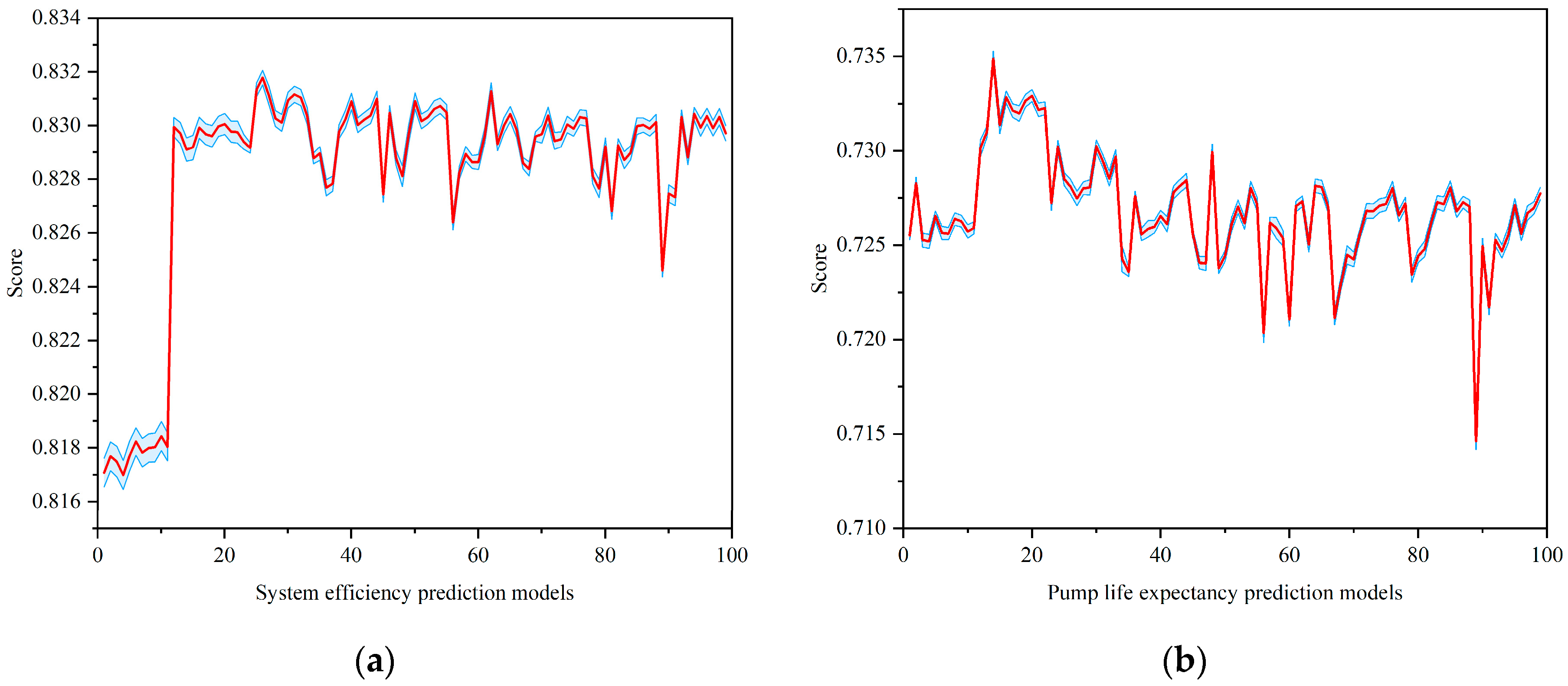
Hyperparameter optimization is important for improving the accuracy of the model. The grid search cross-validation method is used to optimize the parameters of the Random Forest prediction model [41,42,43]. A total of 99 prediction models are trained with different hyperparameters using 4000 well data from the training set. Then, 500 well data from the validation set are used to predict the performance of the trained models, and the optimal hyperparameters are determined based on the evaluation index of the prediction results of different models. The main hyperparameters of the Random Forest include the maximum depth of the decision tree and the number of decision trees in each forest model. The parameter options for the maximum depth of the decision tree are 3, 5, 8, 12, 15, 25, 30, 40, and 50. The parameter options for the number of decision trees include 50, 80, 100, 120, 150, 200, 300, 500, 800, 1200, and 1500. A 5-fold cross-validation is performed, and the scores of each model are calculated as shown in Figure 4.
The red curve represents the average prediction results using 5-fold cross-validation, while the blue area indicates the variance. From Figure 4, it can be seen that the optimal parameter results for system efficiency prediction are a decision tree maximum depth of 8 and 120 decision trees, resulting in the best performance of 0.83. For pump life expectancy prediction, the optimal parameter results are a decision tree maximum depth of 5 and 100 decision trees, with the best performance reaching 0.73.
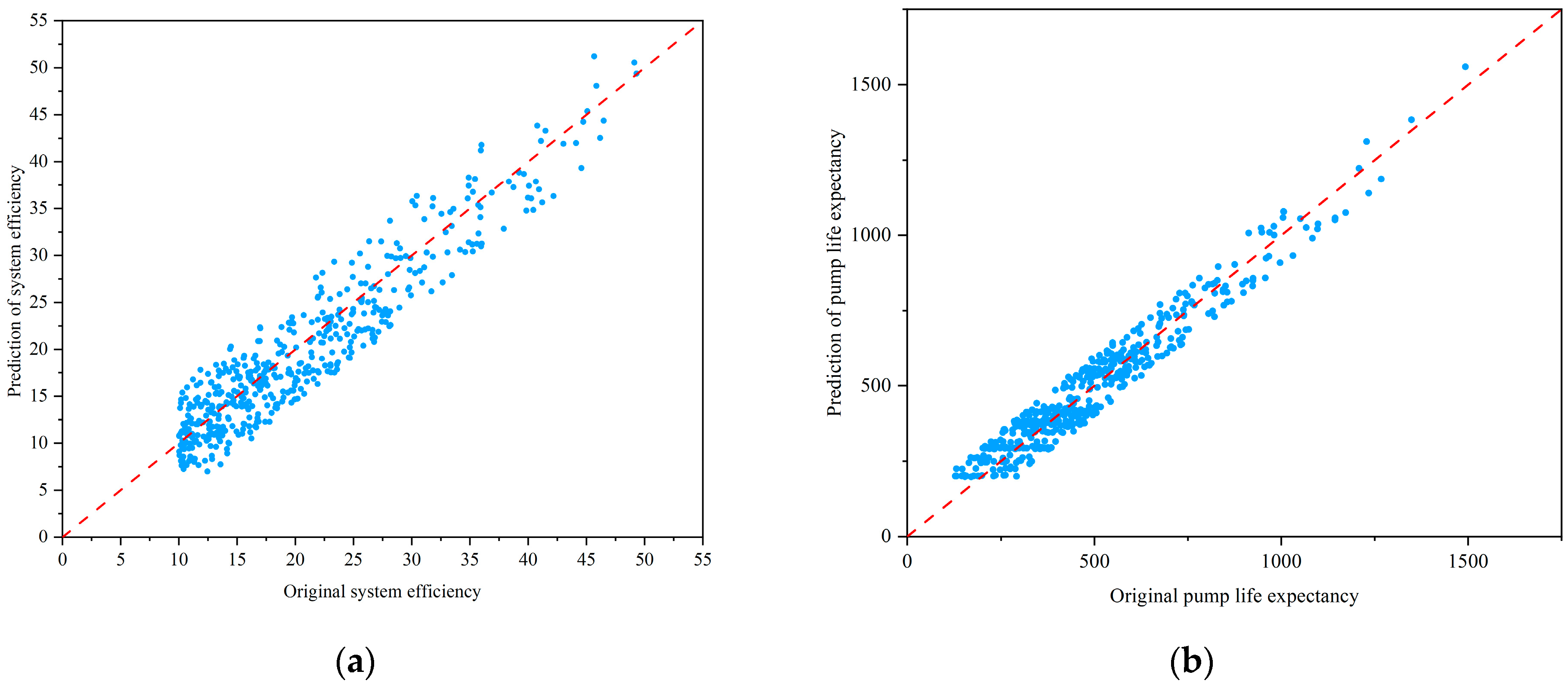
After training the models, to validate the performance of the prediction models, the test set samples are used as input data, and the predicted results are compared with the original data, as shown in Figure 5.
The horizontal axis represents the actual values, and the vertical axis represents the predicted values. The red line represents instances where the actual values equal the predicted values. When the data points on the graph are more concentrated around the red line, it indicates that the predicted results are closer to the actual values, indicating a better performance of the prediction model. The predicted calculation results are shown in Table 1.
As can be seen from Table 1, the model fitting effect is good at this time, which proves that the model has excellent performance, good generalization ability and certain applicability.

6.2. Optimization Performance Evaluation of Lifting System Design Parameters

Two wells were randomly selected and the relevant data are shown in Table 2.
During the optimization process, system efficiency and pump life expectancy are not taken from field measurements but are instead predicted by the trained Random Forest model for each candidate design. The CMA-ES algorithm relies exclusively on these model-predicted values to evaluate and update lifting parameters. After an optimized scheme is obtained, it is implemented in the field, and new operational data are collected to verify the actual improvement. Thus, predictive modeling drives the optimization, while field data are used only for post-optimization validation.
From Table 2, it can be seen that the selected lifting system has low efficiency and a short service life for the lifting design. To address this issue, the CMA-ES algorithm is used to optimize the design parameters of the lifting system. The specific implementation steps are as follows:
(1) Objective function: The objective is to maximize the system efficiency and pump life expectancy, two performance indicators of the lifting system. The multi-objective problem is transformed into a single-objective problem using linear weighted summation. The system efficiency and pump life expectancy are assigned appropriate weight coefficients based on their importance, and their product is used as the new objective function. A higher value of the objective function indicates a better optimized lifting system design.
(2) Input optimization variable parameters include determining stroke, frequency, pump setting depth, pump diameter as the four optimization variables. Considering the actual oilfield conditions, the range of variation for each design parameter is specified, setting upper and lower limits for each optimization variable. To prevent excessive search range, for parameters such as stroke, frequency, and pump setting depth, the stroke range is set from 1m to 9m, the number of strokes range is from 0.8 times·min−1 to 9 times·min−1, and the pump setting depth range is from 350 m to 3400 m. The range is set to be 0.8 to 1.2 times the selected well’s indicator. For the selected 5000 wells, commonly used pump diameters are: 38, 44, 50, 56, 57, 63, 70, 83, 95, and 105 mm. The pump diameter range is set to vary within 1 to 2 sizes based on the original well pump diameter data.
(3) Handling strategy for constraint conditions: A penalty term is added to the objective function ST (H, F, B, P, M) to construct a penalized adaptability function eval (H, F, B, P, M). I. For a portion of wells, the submersion depth ranges from 300 m to 1150 m. According to practical mining applications, excessive or insufficient submersion depth will reduce pump efficiency. There theoretically exists a reasonable submersion depth, determined to be within 200 m to 500 m. II. Displacement constraints: The product of pump diameter, stroke, frequency remains approximately constant before and after optimization. Therefore, a penalty term is added to the objective function:
S T e v a l   ( H , F , B , P , M ) = S T   ( H , F , B , P , M ) + Q   ( H , F , B , P , M )
where Q is the penalty function, when the parameters do not meet the specified conditions, Q = −0.9ST; otherwise Q = 0.
(4) Initializing CMA-ES algorithm parameters: Initial values, step size, boundary constraints, population size, and number of iterations are set. The initial values are the means of each parameter, the step size is 0.1, the boundary constraints are the upper and lower limits determined in step 1, the population size is 10, and the number of iterations is 100.
(5) Judgment: The maximum fitness value and the average fitness value change little and tend to stabilize. If the conditions are met, the optimal parameters are output. Otherwise, the calculation continues until the conditions are satisfied, resulting in the lifting system parameters when the predicted pump life expectancy and system efficiency are optimal.
During the optimization process, system efficiency and pump life are obtained from the predictive model trained on historical field data, because the optimized design has not yet been applied in the field. After the optimized scheme is put into actual operation, real field data are collected and used directly to evaluate the actual system efficiency and pump life, which provides the basis for validating the improvement achieved by the optimization.
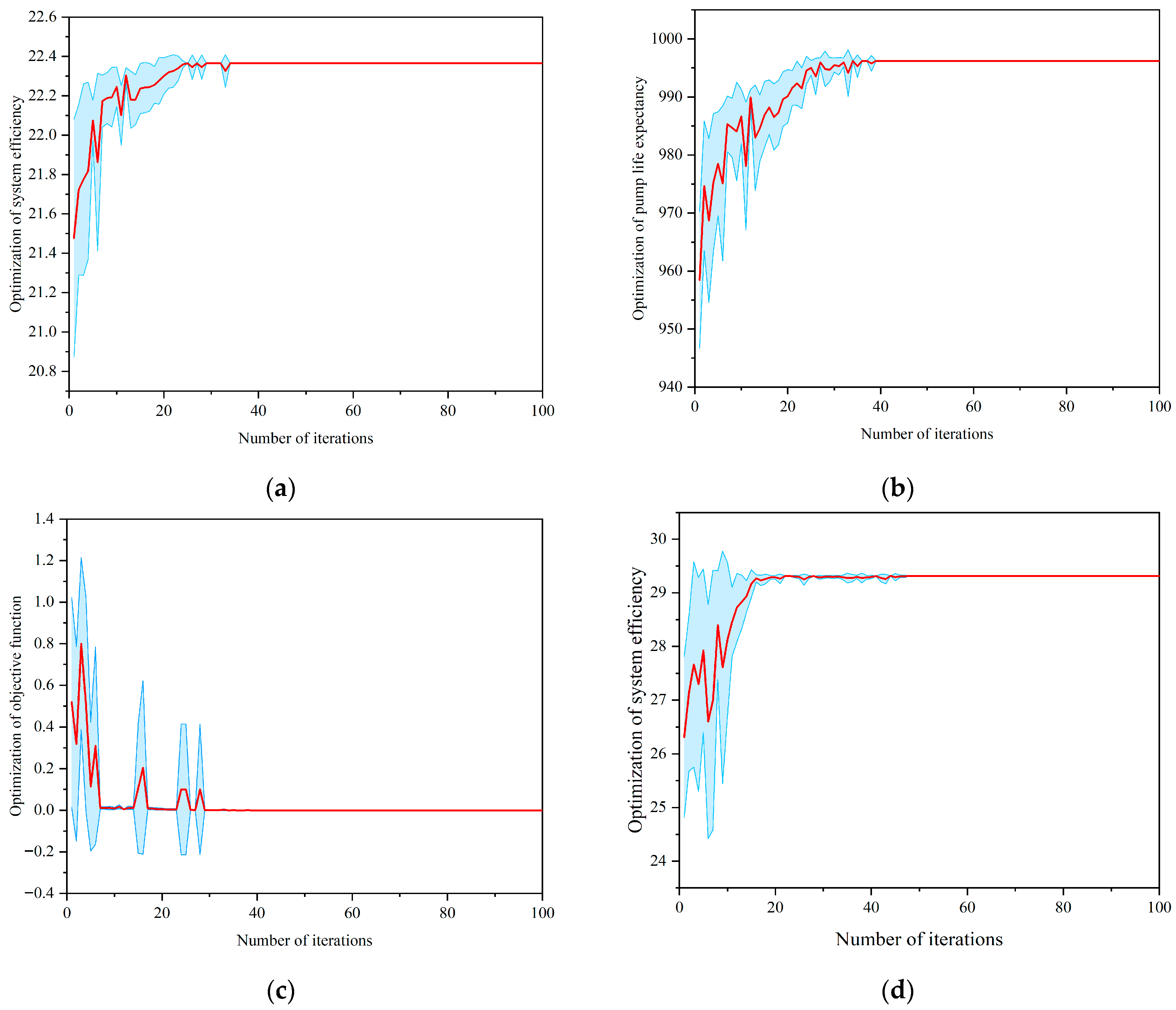
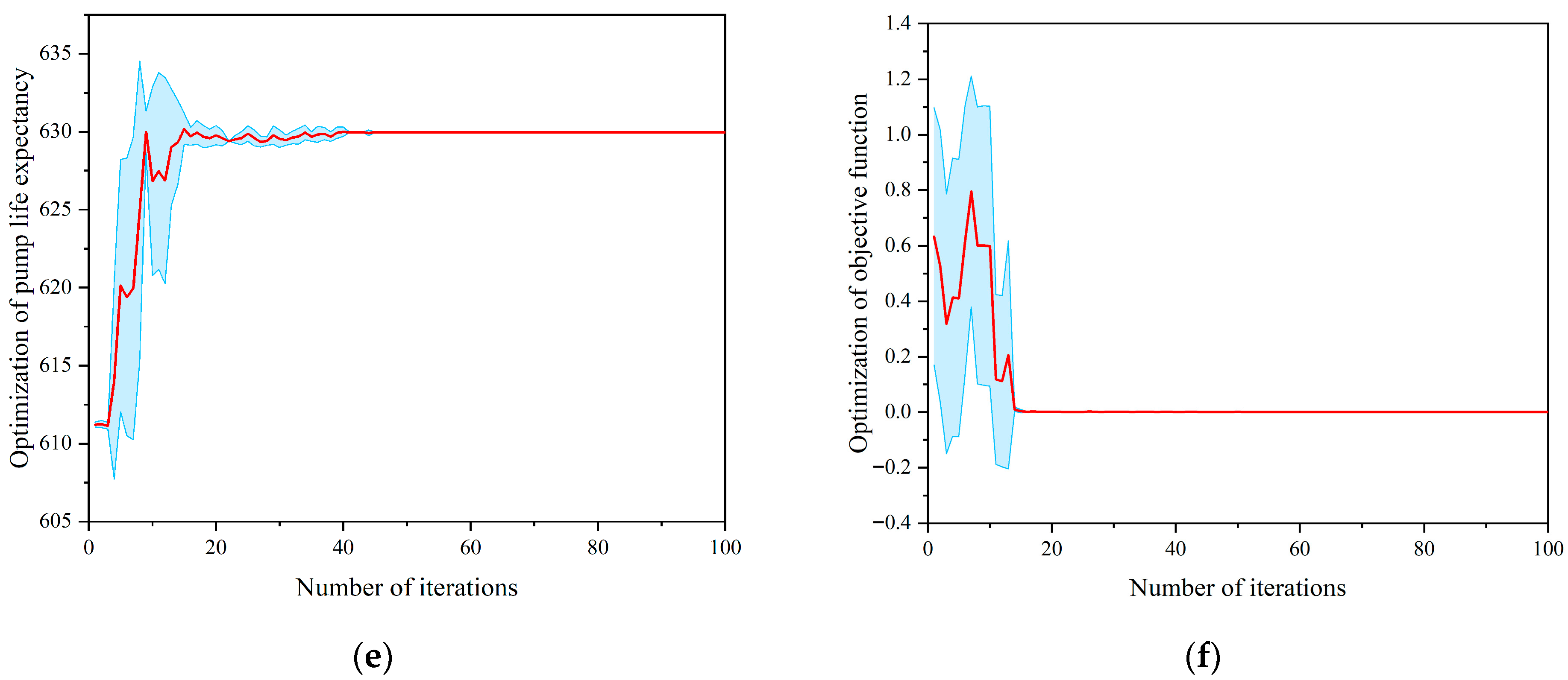
The efficiency and pump life expectancy under various parameter combinations are calculated, and the optimal objective function values are normalized. Here, 0 represents the global optimal value for the problem, while 1 represents the worst solution. This process yields the combination of lifting system design parameters at the optimal system efficiency and pump life expectancy, as shown in the optimization process in Figure 6.
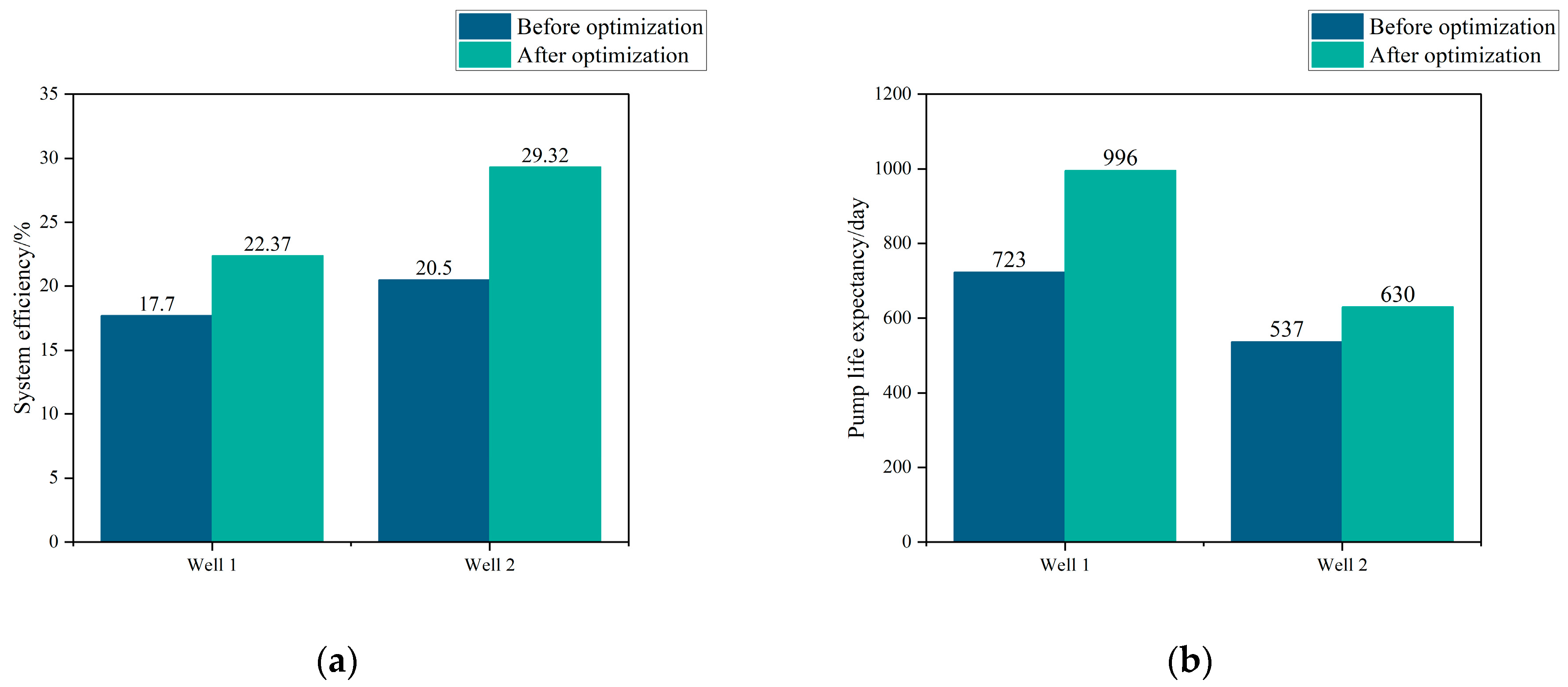
The red curve represents the average of the optimization results of 10 populations in each generation, and the blue area indicates the standard deviation. From Figure 6, it can be observed that the optimization results for system efficiency and pump life expectancy exhibit oscillations followed by an overall increase. The optimization results of the objective function eventually converge, yielding the optimization results as shown in Figure 7.
From Table 3, it can be seen that based on the optimized combination data, adjustments were made to the design parameters of the lifting system. Specifically, the pump setting depth was increased, stroke was increased, frequency was decreased, and pump diameter was enlarged. As a result of these optimizations, the average system efficiency increased from 19.1% to 25.85%, representing an expected improvement of 6.75%. The pump life expectancy also increased from 630 days to 813 days, indicating an expected improvement of 29%. These improvements result mainly from the optimized parameters operating within more suitable ranges. The new combination of stroke, frequency, pump diameter, and pump setting depth leads to a more stable rod-string load and more consistent pump-intake conditions. This reduces load fluctuations and improves pump filling, which helps prevent gas interference and fluid pounding. As a result, the pumping system runs more smoothly, producing higher efficiency and longer pump life.

7. Conclusions

(1) A smart optimization algorithm model for the design parameters of the oil well lifting system was proposed, aiming to maximize system efficiency and pump life expectancy. Parameters such as stroke, frequency, pump setting depth, and pump diameter were jointly optimized to enhance both system efficiency and pump life expectancy after optimization. Case studies show efficiency gains of 6.75% and pump life improvements of 29% through coordinated parameter optimization. This method holds theoretical significance and practical value, providing references and guidance for the design and management of oil well lifting systems.
(2) This study presents a new approach and means for optimizing the design of lifting systems, offering valuable insights and references for the efficient utilization of big data in oilfields and the enhancement of oilfield productivity. By adjusting the weight assigned to specific indicators based on practical needs, the effectiveness of those indicators can be enhanced.
(3) Future work will aim to improve the generalization and transparency of the model. This includes expanding the dataset to cover a wider range of geological and operating conditions, incorporating physical constraints where appropriate, and exploring multi-objective algorithms that can provide a more complete description of the trade-offs. In addition, comparative testing with methods such as Artificial Neural Networks (ANN) and Response Surface Models (RSM) will be carried out to further assess the performance of the proposed approach.

Author Contributions

Conceptualization, X.W. and Y.Z.; methodology, X.W., Y.Z., Y.X., L.C., W.Y., M.L. and Y.W.; software, X.W. and Y.Z.; validation, X.W., Y.Z. and L.C.; formal analysis, W.Y.; resources, X.W., Y.X., L.C., W.Y., Y.W. and M.L.; data curation, Y.X.; writing—original draft preparation, Y.Z.; writing—review and editing, X.W.; visualization, X.W.; supervision, X.W.; funding acquisition, X.W. All authors have read and agreed to the published version of the manuscript.

Funding

This research was funded by the National Natural Science Foundation of China (No. 52204027), the Qinglan Project of Jiangsu Province of China (2024) and the Postgraduate Research & Practice Innovation Program of Jiangsu (No. SJCX24_3241).

Data Availability Statement

The original contributions presented in this study are included in the article. Further inquiries can be directed to the corresponding author.

Conflicts of Interest

The authors declare no conflicts of interest.

References

  1. Greg, S. Technology Focus: Artificial Lift (March 2022). J. Pet. Technol. 2022, 74, 57–58. [Google Scholar] [CrossRef]
  2. Gan, X.; Jian, J.; Pavesi, G.; Yuan, S.; Wang, W. Application of intelligent methods in energy efficiency enhancement of pump system: A review. Energy Rep. 2022, 8, 11592–11606. [Google Scholar] [CrossRef]
  3. Khormali, A.; Sharifov, A.R.; Torba, D.I. The control of asphaltene precipitation in oil wells. Pet. Sci. Technol. 2018, 36, 443–449. [Google Scholar] [CrossRef]
  4. Cao, L.; Lv, M.; Li, C.; Sun, Q.; Wu, M.; Xu, C.; Dou, J. Effects of Crosslinking Agents and Reservoir Conditions on the Propagation of Fractures in Coal Reservoirs During Hydraulic Fracturing. Reserv. Sci. 2025, 1, 36–51. [Google Scholar] [CrossRef]
  5. Wu, J.; Ansari, U. From CO2 Sequestration to Hydrogen Storage: Further Utilization of Depleted Gas Reservoirs. Reserv. Sci. 2025, 1, 19–35. [Google Scholar] [CrossRef]
  6. Hansena, B.; Tolbertb, B.; Vernona, C.; Hedengrena, J.D. Model predictive automatic control of sucker rod pump system with simulation case study. Comput. Chem. Eng. 2019, 121, 265–284. [Google Scholar] [CrossRef]
  7. Xing, M.; Zhou, L.; Zhang, C.; Xue, K.; Zhang, Z. Simulation analysis of nonlinear friction of rod string in sucker rod pumping system. J. Comput. 2019, 14, 091008. [Google Scholar] [CrossRef]
  8. Lv, X.; Wang, H.; Zhang, X.; Liu, Y.; Chen, S. An equivalent vibration model for optimization design of carbon/glass hybrid fiber sucker rod pumping system. J. Pet. Sci. Eng. 2021, 207, 109148. [Google Scholar] [CrossRef]
  9. He, D. Study on the Combination of Pump Rod Pipe in Complex Structure. Sci. Program. 2022, 2022, 3041911. [Google Scholar] [CrossRef]
  10. Langbauer, C.; Langbauer, T.; Fruhwirth, R.; Mastobaev, B. Sucker rod pump frequency-elastic drive mode development–from the numerical model to the field test. Liq. Gaseous Energy Resour. 2021, 1, 64–85. [Google Scholar] [CrossRef]
  11. Jalikop, S.V.; Albishini, R.; Freudenberger, M.; Scheichl, B.; Langbauer, C.; Eder, S.J. An Extended Computational Fluid Dynamics Model and Its Experimental Validation to Improve Sucker Rod Pump Operation and Design. SPE J. 2025, 30, 6249–6261. [Google Scholar] [CrossRef]
  12. Gu, X.; Liao, Z.; Hu, S.; Yi, J.; Li, T. Decision Parameter Optimization of Beam Pumping Unit Based on BP Networks Model. In Fuzzy Information & Engineering and Operations Research & Management; Springer: Berlin/Heidelberg, Germany, 2014; pp. 13–20. [Google Scholar] [CrossRef]
  13. Han, G.; Zhang, H.; Ling, K. The optimization approach of casing gas assisted rod pumping system. J. Nat. Gas. Sci. Eng. 2016, 32, 205–210. [Google Scholar] [CrossRef]
  14. Shi, J.; Chen, S.; Zhang, X.; Zhao, R.; Liu, Z.; Liu, M.; Zhang, N.; Sun, D. Artificial lift methods optimising and selecting based on big data analysis technology. In Proceedings of the International Petroleum Technology Conference 2019, Beijing, China, 26–28 March 2019; p. D011S0R03. [Google Scholar] [CrossRef]
  15. Feng, D.; Qi, Y.; Yu, Y.; Zhu, H. Neural Network-Based Beam Pumper Model Optimization. Comput. Intell. Neurosci. 2022, 2022, 8562387. [Google Scholar] [CrossRef] [PubMed]
  16. Chu, X.; Wang, X.; Xie, Y.; Xing, G.; Chen, L. Association rules mining for long uptime sucker rod pumping units. Reliab. Eng. Syst. Saf. 2024, 245, 110026. [Google Scholar] [CrossRef]
  17. Zhao, R.; Zhang, X.; Liu, M.; Shi, J.; Su, L.; Shan, H.; Sun, C.; Miao, G.; Wang, Y.; Shi, L.; et al. Production optimizaton and application of combined artificial-lift systems in deep oil wells. In Proceedings of the SPE Middle East Artificial Lift Conference and Exhibition 2016, Manama, Kingdom of Bahrain, 30 November–1 December 2016; p. D021S07R03. [Google Scholar] [CrossRef]
  18. Almedallah, M.K.; Clark, S.; Walsh, S.D.C. Schedule Optimization To Accelerate Offshore Oil Projects While Maximizing Net Present Value in the Presence of Simultaneous Operations, Weather Delays, and Resource Limitations. SPE Prod. Oper. 2022, 37, 54–71. [Google Scholar] [CrossRef]
  19. Alcántara, A.; Ruiz, C. On data-driven chance constraint learning for mixed-integer optimization problems. Appl. Math. Model. 2023, 121, 445–462. [Google Scholar] [CrossRef]
  20. Temizel, C.; Canbaz, C.H.; Betancourt, D.; Ozesen, A.; Acar, C.; Krishna, S.; Saputelli, L. A comprehensive review and optimization of artificial lift methods in unconventionals. In Proceedings of the SPE Annual Technical Conference and Exhibition 2020, Virtual, 5–7 October 2020; p. D041S53R08. [Google Scholar] [CrossRef]
  21. Le, V.; Tran, S. Hybrid Electrical-Submersible-Pump/Gas-Lift Application to Improve Heavy Oil Production: From System Design to Field Optimization. J. Energy Resour. Technol. 2022, 144, 083006. [Google Scholar] [CrossRef]
  22. Takacs, G. Ways to obtain optimum power efficiency of artificial lift installations. In Proceedings of the SPE Oil and Gas India Conference and Exhibition 2010, Mumbai, India, 20–22 January 2010; p. SPE-126544-MS. [Google Scholar] [CrossRef]
  23. Aydin, H.; Merey, S. Design of Electrical Submersible Pump system in geothermal wells: A case study from West Anatolia, Turkey. Energy 2021, 230, 120891. [Google Scholar] [CrossRef]
  24. Shi, Y.; Xia, Y.; Zhang, Y.; Yao, Z. Intelligent identification for working-cycle stages of excavator based on main pump pressure. Autom. Constr. 2020, 109, 102991. [Google Scholar] [CrossRef]
  25. Li, M.; Liu, J.; Xia, Y. Risk Prediction of Gas Hydrate Formation in the Wellbore and Subsea Gathering System of Deep-Water Turbidite Reservoirs: Case Analysis from the South China Sea. Reserv. Sci. 2025, 1, 52–72. [Google Scholar] [CrossRef]
  26. Ning, Y.; Schumann, H.; Jin, G. Application of Data Mining to Small Data Sets: Identification of Key Production Drivers in Heterogeneous Unconventional Resources. SPE Reserv. Eval. Eng. 2023, 26, 411–421. [Google Scholar] [CrossRef]
  27. Chris, C. Machine-Learning Approach Optimizes Well Spacing. J. Pet. Technol. 2021, 73, 44–45. [Google Scholar] [CrossRef]
  28. Simoes, V.; Maniar, H.; Abubakar, A.; Zhao, T. Comparative study of machine-learning-based methods for log prediction. Petrophysics 2023, 64, 192–212. [Google Scholar] [CrossRef]
  29. Chan, Y.H. Biostatistics 104: Correlational analysis. Singap. Med. J. 2003, 44, 614–619. [Google Scholar]
  30. Chris, C. Machine-Learning Model Improves Gas Lift Performance and Well Integrity. J. Pet. Technol. 2022, 74, 83–85. [Google Scholar] [CrossRef]
  31. Ali, S.; Afshin, T.; Mahsheed, R.; Madiyar, K.; Ingkar, A. Artificial neural network, support vector machine, decision tree, random forest, and committee machine intelligent system help to improve performance prediction of low salinity water injection in carbonate oil reservoirs. J. Pet. Sci. Eng. 2022, 219, 111046. [Google Scholar] [CrossRef]
  32. Tao, J.; Yin, X.; Yao, X.; Cheng, Z.; Yan, B.; Chen, G. Prediction of NH3 and HCN yield from biomass fast pyrolysis: Machine learning modeling and evaluation. Sci. Total Environ. 2023, 885, 163743. [Google Scholar] [CrossRef] [PubMed]
  33. Olumegbon, I.A.; Alade, I.O.; Oyedeji, M.O.; Qahtan, T.F.; Bagudu, A. Development of machine learning models for the prediction of binary diffusion coefficients of gases. Eng. Appl. Artif. Intell. 2023, 123, 106279. [Google Scholar] [CrossRef]
  34. Karmakar, B.; Kumar, A.; Mallipeddi, R.; Lee, D.-G. CMA-ES with exponential based multiplicative covariance matrix adaptation for global optimization. Swarm Evol. Comput. 2023, 79, 101296. [Google Scholar] [CrossRef]
  35. Zaid, A.; Mohammad, S. (μ + λ) Evolution strategy algorithm in well placement, trajectory, control and joint optimisation. J. Pet. Sci. Eng. 2019, 177, 1042–1058. [Google Scholar] [CrossRef]
  36. Weng-Hooi, T.; Junita, M.-S. MO-NFSA for solving unconstrained multi-objective optimization problems. Eng. Comput. 2022, 38, 2527–2548. [Google Scholar] [CrossRef]
  37. Demmelash Mollalign, M.; Berhanu Guta, W.; Allen, R. Solving multi-objective linear fractional decentralized bi-level decision-making problems through compensatory intuitionistic fuzzy mathematical method. J. Comput. Sci. 2023, 71, 102075. [Google Scholar] [CrossRef]
  38. Peng, Y.; Wu, L.; Shiue, M. Finite time synchronization of the continuous/discrete data assimilation algorithms for Lorenz 63 system based on the back and forth nudging techniques. Results Appl. Math. 2023, 20, 100407. [Google Scholar] [CrossRef]
  39. Humphries, T.D.; Haynes, R.D. Joint optimization of well placement and control for nonconventional well types. J. Pet. Sci. Eng. 2015, 126, 242–253. [Google Scholar] [CrossRef]
  40. Carvalho, G.d.A.; Minnett, P.J.; Ebecken, N.F.F.; Landau, L. Machine-Learning Classification of SAR Remotely-Sensed Sea-Surface Petroleum Signatures—Part 1: Training and Testing Cross Validation. Remote Sens. 2022, 14, 3027. [Google Scholar] [CrossRef]
  41. Massimo, C.; Luigi, B.; Gino, C.; Giovanni, G. Exploring performance and robustness of shallow landslide susceptibility modeling at regional scale using different training and testing sets. Environ. Earth Sci. 2023, 82, 161. [Google Scholar] [CrossRef]
  42. Adnan, M.; Alarood, A.A.S.; Uddin, M.I.; Rehman, I.U. Utilizing grid search cross-validation with adaptive boosting for augmenting performance of machine learning models. PeerJ Comput. Sci. 2022, 8, e803. [Google Scholar] [CrossRef]
  43. Sweeti, S.; Balasubramanian, S.; Ramasamy, D.; Mohammed, Y. COVID-19 cases prediction using SARIMAX Model by tuning hyperparameter through grid search cross-validation approach. Expert. Syst. 2023, 40, e13086. [Google Scholar] [CrossRef]
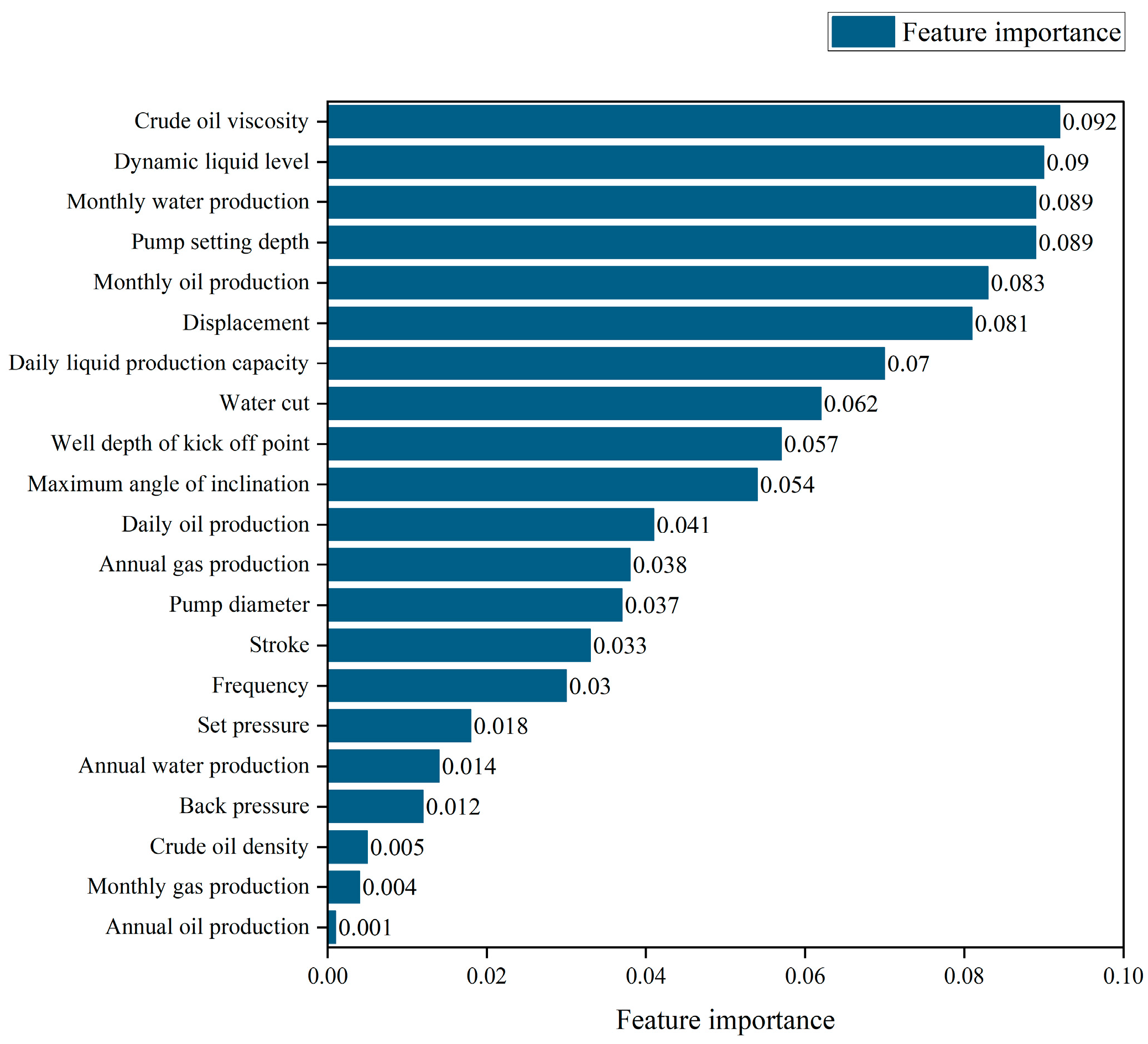
Figure 1. Feature importance ranking.
Processes 13 03871 g001
Figure 2. Correlation analysis.
Processes 13 03871 g002
Figure 3. Optimization workflow of lifting system design parameters.
Processes 13 03871 g003
Figure 4. Optimization performance of the prediction models. (a) system-efficiency prediction model optimization; (b) pump life-expectancy prediction model optimization.
Processes 13 03871 g004
Figure 5. Compares the predicted values with the actual values. (a) Comparison of system efficiency test set; (b) Compares the predicted values with the actual values.
Processes 13 03871 g005
Figure 6. The optimization process. (a) Well 1 optimization of system efficiency process; (b) Well 1 optimization of pump life expectancy; (c) Well 1 optimization of objective function; (d) Well 2 optimization of system efficiency; (e) Well 2 optimization of pump life expectancy; (f) Well 2 optimization of objective function.
Processes 13 03871 g006aProcesses 13 03871 g006b
Figure 7. Optimization search process. (a) Comparison of system efficiency before and after optimization; (b) Comparison of pump life expectancy before and after optimization.
Processes 13 03871 g007
Table 1. Predicts the computational results.
Evaluating IndicatorSystem EfficiencyPump Life Expectancy
Training set R20.930.80
Validation set R20.830.73
Test set R20.800.71
Table 2. Production Parameters.
Manufacturing ParameterWell 1Well 2Manufacturing ParameterWell 1Well 2
Dynamic liquid level/m1002987Well depth of kick off point/m584.76747.27
Crude oil viscosity/MPa·s11471264Stroke/m4.786.05
Water cut/%81.270.4Pump setting depth/m1032.131094.84
Annual gas production/109 m30.70.21Pump diameter/mm7057
Daily fluid production capacity/t5.72.4Frequency/times·min−111.4
Maximum angle of inclination/°42.628.5System efficiency/%17.720.5
Monthly oil production/107 t3272Pump life expectancy/day723537
Daily oil production capacity/t4.81.6
Table 3. Optimized scheme.
Optimize the WellStroke/mPump Setting Depth/mPump Diameter/mmFrequency/Times·min−1System Efficiency/%Pump Life Expectancy/d
Well 15.711218.58830.8222.37996
Well 24.991250.26571.5429.32630
Disclaimer/Publisher’s Note: The statements, opinions and data contained in all publications are solely those of the individual author(s) and contributor(s) and not of MDPI and/or the editor(s). MDPI and/or the editor(s) disclaim responsibility for any injury to people or property resulting from any ideas, methods, instructions or products referred to in the content.