Article

Operational Flexibility Assessment of Distributed Reserve Resources Considering Meteorological Uncertainty: Based on an End-to-End Integrated Learning Approach

1
Guangdong Power Grid Co., Ltd., China Southern Power Grid, Guangzhou 510080, China
2
State Key Laboratory of Power Transmission Equipment Technology, Chongqing University, Chongqing 400044, China
*
Authors to whom correspondence should be addressed.
Processes 2025, 13(12), 3870; https://doi.org/10.3390/pr13123870 (registering DOI)
Submission received: 21 October 2025 / Revised: 18 November 2025 / Accepted: 26 November 2025 / Published: 1 December 2025
(This article belongs to the Special Issue Modeling, Optimization, and Control of Distributed Energy Systems)

Abstract

In the context of the rapid development of renewable energy and frequent extreme weather, accurate evaluation of the backup operation flexibility of multiple distributed resources is a prerequisite for improving the resilience of power systems. However, it is difficult to consider the detailed model of each distributed resource and evaluate its regulation ability in the operation of power systems because of the small number of distributed resources. Therefore, this paper first quantifies the capacity boundaries of distributed reserve resources on the power generation, load, and energy storage sides under different meteorological conditions through economic self-dispatching optimization and Minkowski aggregation methods. Subsequently, the maximum correlation–minimum redundancy (mRMR) principle and Granger causality test are combined to reduce the dimensionality of high-dimensional meteorological features. Finally, the stacking ensemble learning method is introduced to build an end-to-end modelling framework from multi-source weather input to reserve capability prediction. The results show that (1) the reserve capacity of multivariate distributed resources has significant intra-day and intra-day periodicity and seasonal differences; (2) the mRMR algorithm considering the Granger causality test can capture the correlation and causality between high-dimensional meteorological features and reserve capabilities, and the obtained features are more explanatory; (3) the average R2 of the stacking model in both upper-reserve and lower-reserve predictions reaches 0.994. In terms of computational efficiency, the training time of the proposed model is 130.85 s for upper-reserve prediction and 133.71 s for lower-reserve prediction, which is significantly lower than that of conventional hybrid models while maintaining stable performance under extreme meteorological conditions such as high temperatures and strong winds; (4) compared with integration methods such as simple averaging and error weighting, the stacking integration strategy proposed in this paper remains stable in the mean and variance of prediction results, verifying its comprehensive advantages in structural design and performance integration.

1. Introduction

1.1. Motivation

Driven by the “dual-carbon” target, China’s energy structure has accelerated its transition to a cleaner and lower-carbon environment, with the rapid expansion of installed renewable energy sources such as wind power and photovoltaic power, providing important support for the achievement of SDG13 [1]. However, the stochastic nature of new energy generation and the volatility of load demand together exacerbate the uncertainty on both sides of the source and load [2,3]. This has led to a significant increase in the difficulty of balancing the dynamics of power systems. The traditional model of relying on conventional power sources to provide backup is no longer able to meet the flexibility needs of a high proportion of renewable energy sources connected to the grid [4]. There is an urgent need to build a diversified reserve resource system and to explore the regulation potential of various types of resources in order to alleviate the problem of insufficient reserve capacity and enhance the margin of safe operation of power systems.
As a key supplement to support the backup flexibility of power systems, distributed resources are increasingly becoming an important pillar to enhance a power system’s regulating capability and emergency protection level due to their advantages of rapid response, strong regulating capability, and flexible layout [5]. Typical distributed reserve resources include distributed energy storage [6], electric vehicles [7], air-conditioning load [8], etc. Against the background of large-scale deployment of intelligent terminals and energy management systems, the aggregation and control of user-side resources has good technical feasibility and economic rationality [9]. However, distributed resources naturally have the attributes of multi-source heterogeneity, wide spatial distribution, and strong dynamic characteristics, which bring significant challenges to their cooperative control and scheduling as reserve resources. On the one hand, its response capability is highly sensitive to the meteorological environment, especially under extreme weather conditions, which is prone to performance degradation or even unavailability [10,11]. On the other hand, the existing reserve capacity assessment methods based on planning optimization have high computational complexity, low solution efficiency, and difficulty in dynamically adapting to meteorological changes in the face of multiple types and large-scale distributed resources [12,13]. Moreover, such approaches usually rely on centralized data collection and control architectures, making it difficult to take into account user-side privacy protection [14]. In this regard, this paper aims to address the following two key scientific questions: (1) How can the reserve response of multiple types of distributed resources be systematically characterized under different meteorological conditions, and how can their meteorological sensitivity and dynamic availability be quantified? (2) How can a generalized data-driven model be constructed with both high efficiency and privacy protection to realize the rapid assessment of the security margins of distributed reserve resources for grid operation?

1.2. Literature Review

1.2.1. Impact of Meteorological Uncertainty on the Operational Characteristics of Reserve Resources

The large-scale connection of a high proportion of renewable energy sources makes a power system increasingly dependent on meteorological conditions, which drives scholars to analyze the reserve response characteristics and scheduling strategies of multiple types of resources, including source, network, load and storage, under meteorological uncertainty [15]. On the power generation side, meteorological factors cause significant intermittency and volatility in the output of renewable energy sources, leading to considerable uncertainty in their adjustable output boundaries. Existing studies have modelled the dynamic output characteristics of wind and photovoltaic systems under varying weather conditions [16], the boundaries of forecasting errors [17], and flexible operation strategies [18], aiming to comprehensively capture their operational features, including adjustable output range, ramp rate limits, and frequency response capabilities [18]. Demand-side resources are decentralized and highly responsive, and their reserve response capacity is jointly affected by user behaviour and meteorological changes, with typical temperature threshold response characteristics and response duration constraints, and they often participate in load shedding or shifting through demand response [19,20,21,22,23]. Grid-side resources provide backup for a power system through line transmission capacity and contact line transmission power, and scholars often propose risk-hedging strategies through the AC-DC interconnection system to mitigate the effects of meteorological uncertainty through the backup support function of regional contact lines [24,25,26]. Energy storage resources, such as distributed storage systems, electric vehicle fleets, and mobile energy storage units, have become a crucial support for time-sensitive backup regulation during extreme weather events due to their energy buffering and fast response capabilities [27]. Existing studies [28,29,30] have mainly characterized their operational boundary features under different meteorological conditions in terms of regulation speed, response delay, and energy capacity limitations.
In summary, existing studies have been carried out to portray the regulation boundaries of multiple types of reserve resources under meteorological uncertainties and to promote the coordinated scheduling of resources on multiple sides of the source, network, load, and storage. However, the current research focuses on the independent modelling of single or several types of resources and lacks the understanding of the joint operation characteristics of multi-source heterogeneous resources under meteorological perturbations, and the influence of reserve resource clusters on the security margin boundary of power grid operation needs to be further explored.

1.2.2. Operational Flexibility Evaluation of Multi-Source Distributed Reserve Resources

Distributed resources have a certain degree of flexibility due to their large-scale access, and quantifying and evaluating the regulation capability of multi-source distributed resources have become important bases for guaranteeing the safe operation of a power system [31]. Studies have been conducted on distributed reserve resource assessment mainly through optimal modelling or artificial intelligence methods [32,33]. Optimization-based modelling approaches are mainly based on the physical characteristics of resources and operational constraints to construct self-scheduling or coordinated scheduling models with the objective of maximizing economy and reserve capacity. Typical modelling approaches include mixed-integer linear programming (MILP) [34,35,36], robust optimization [37,38], two-stage stochastic optimization [39], etc. The advantage of these methods is that they can finely portray resource regulation characteristics and operation boundaries in the face of large-scale resource clusters and high-frequency dynamic perturbations, but there are problems such as complex modelling, high computational overhead, and weak on-line adaptive capacity. With the development of artificial intelligence, data-driven assessment methods have gradually become an effective alternative in application scenarios with high modelling complexity and abundant data access [40]. This type of methodology enables rapid prediction and dynamic assessment of reserve potential by learning the statistical patterns between meteorological data, operational status, and historical reserve behaviour [41]. Common methods include GRU [42], LSTM [43], and other neural network models, as well as random forest [44], gradient boosting tree [45], and LightGBM [46]. However, it should be noted that data-driven methods are highly dependent on data quality and feature selection, and there are still some accuracy and stability deficiencies in weather-alternative scenarios due to the high feature dimensionality and the small number of samples.
In summary, the optimization modelling approach has limited accuracy in portraying meteorological perturbations and dynamic availability, which is difficult to adapt to the real-time assessment of large-scale heterogeneous resources; whereas the data-driven approach has good prediction capability but lacks physical boundary constraints and systematic consideration of feature selection and causal structure, which affects the interpretability and reliability of the model. Against the background of the significant increase in the demand for distributed resource backup, there is an urgent need for a unified methodological framework that integrates the advantages of physical modelling and data-driven capabilities, so as to provide a credible auxiliary decision-making basis for the participation of distributed resources in system scheduling.

1.2.3. Research Gap

Table 1 shows the differences between our study and previous studies. Despite the extensive research on individual types of reserve resources and their operational characteristics under meteorological uncertainty, there remain several critical gaps. First, most existing studies focus on single-type or a few types of resources in isolation, lacking a comprehensive understanding of the joint operational dynamics of multi-source heterogeneous reserve resources under varying weather conditions. Second, while optimization-based approaches provide clear physical and operational boundaries, they struggle with high-dimensional, large-scale, and real-time scenarios, limiting their practical applicability. Third, data-driven approaches, although capable of rapid prediction and dynamic assessment, often suffer from insufficient feature selection, limited consideration of causal relationships, and a lack of physical interpretability. To address these gaps, the present study aims to develop a unified framework that combines optimization-based physical modelling and data-driven predictive capabilities. This framework systematically evaluates multi-source distributed reserve resources under meteorological uncertainty, selects interpretable and relevant meteorological features, and constructs an end-to-end learning model to accurately predict reserve capacity. The proposed approach not only improves the understanding of joint operational behaviours but also enhances practical applicability for real-time scheduling and resource management in complex power systems.

1.3. Contributions

To address the limitations of existing studies in assessing the operational flexibility of distributed reserve resources, this study proposes a multi-source, meteorology-aware evaluation and prediction framework for distributed reserve capability. The proposed framework serves as both a planning tool and an operational decision-support solution. At the planning level, it provides capacity allocation and redundancy configuration guidance for system integrators and distribution companies. At the operational level, it supports system operators and utilities by dynamically evaluating and scheduling distributed reserves under meteorological disturbances, thus enhancing flexibility and operational resilience. Specifically, this study firstly combed multiple types of distributed resources on the generation, load, and storage sides, constructed an economic self-scheduling model integrating meteorological uncertainties, and used Minkowski aggregation methods to unify the reserve capacity boundaries of the resource clusters. Secondly, we combine the principle of minimum redundancy–maximum relevance (mRMR) and Granger causality test to downscale the high-dimensional meteorological features to improve the model modelling efficiency and physical interpretation. Finally, we construct an end-to-end integrated learning framework based on stacking to achieve efficient prediction from multi-source meteorological features to reserve capacity. The marginal contributions of this paper are as follows:
(1)
A distributed reserve capacity response evaluation system for meteorological uncertainty is constructed. This study quantifies the reserve potentials of various resources under different meteorological conditions through optimization modelling and Minkowski aggregation and uniformly portrays the reserve boundaries of distributed resource clusters under different spatial and temporal conditions, so as to provide high-quality samples for the subsequent machine learning modelling.
(2)
A high-dimensional meteorological feature selection method considering correlation and causality is proposed. In this study, minimum redundancy–maximum relevance principle and Granger causality test are combined to construct a subset of features with interpretability and stability between the multidimensional NWP data and the spare capacity, which can enhance the credibility of the data-driven model.
(3)
The integrated weather-reserve learning model is constructed considering the diversity of models. Based on the stacking framework, this study proposes an adaptive selection strategy for base and meta learners that takes into account model diversity and combination performance, which improves the prediction accuracy and generalization ability of the model under high-dimensional, nonlinear weather perturbation conditions for distributed resource reserve potential.

2. Methodology

In order to efficiently assess the responsiveness of distributed reserve resources under meteorological uncertainty, an end-to-end data-driven modelling framework is constructed in this chapter, and the overall approach includes three core components: reserve capacity sample generation, feature screening, and integrated learning modelling. To address the sample scarcity problem, an economic self-dispatch model incorporating meteorological perturbations is constructed to quantify the adjustable boundaries of distributed generation, load, and energy storage resources under different meteorological conditions, and resources are aggregated through Minkowski’s method to form backup capacity training samples. Considering the problem of high dimensionality and high relevance of meteorological features with complex redundancy, a feature screening method combining mRMR and Granger causality test is designed to extract a subset of key features that are highly relevant to reserve capacity and have causal relationships. Finally, this paper constructs a multi-model integrated learning architecture based on stacking to improve the accuracy and generalization performance of reserve capacity prediction under meteorological disturbances by integrating multiple prediction models. The overall research framework is shown in Figure 1.

2.1. Characterization of Reserve Resource Capacity with Meteorological Uncertainty

2.1.1. Operational Modelling of Distributed Power Generations

For the distributed power side, climate uncertainty mainly affects new energy output and changes the reserve regulation boundary, hence, this section mainly considers distributed photovoltaic and distributed wind power [47]. When the wind turbine output is more than 20% of the total rated output, the system can be provided with reserve auxiliary services through load shedding [48]. The day-ahead scheduling centre determines the operational reference values P w i n d , T and load shedding plans for wind farms based on wind power forecasts P w i n d , T f o r e , and issues them to the wind farms. In the event of a system power imbalance, wind turbine generators (WTGs) can provide upward R w i n d , T u p and downward R w i n d , T d o w n reserve capacities. The corresponding operational and reserve constraints are as follows:
P w i n d , T = ( 1 β w i n d , T ) P w i n d , T f o r e
0 β w i n d , T β ¯ w i n d
R w i n d , T u p = β w i n d , T P w i n d , T f o r e
R w i n d , T d o w n = ( β ¯ w i n d β w i n d , T ) P w i n d , T f o r e
where β w i n d , T is the curtailment ratio parameter of wind turbine w at time period T ; β ¯ w i n d is the upper limit of the curtailment ratio for wind turbine w .
The process of providing operational reserve for a PV plant is similar to that for wind power, but the reserve capacity for grid-connected operation is provided by the PV array and the accompanying energy storage unit [49], so that the operational reserve constraints are
0 R s o l a r , T u p P s o l a r , T f o r e P s o l a r , T
0 R s o l a r , T d o w n P s o l a r , T P _ s o l a r , T
where R s o l a r , T u p and R s o l a r , T d o w n denote the upward and downward reserve capacities provided by photovoltaic station at time period T , respectively; P s o l a r , T f o r e and P s o l a r , T represent the day-ahead active power forecast and the operational reference value of PV station at time T , respectively; P _ s o l a r , T is the minimum grid-connected power of PV station.
In addition to the operating reserve constraints, the self-scheduling models of PV and wind power also need to consider the output range constraints, power balance constraints, and ramp rate constraints, etc. The objective function is to maximize economic efficiency, taking into account new energy feed-in revenue and reserve compensation. This approach is similar to the existing literature, for example, Müller [50] considered the model of climbing rate limit + reserve bidding. In addition, the CSP-PV-wind power dispatching model proposed by Xu [51] takes into account uncertainty as well as economic goals.

2.1.2. Operational Modelling of Flexible Loads

For the demand side, incentivised demand response is an effective reserve resource. In times of tight supply/demand balance, the demand side can reduce demand through load shedding (e.g., air conditioning) and load shifting (e.g., electric water heaters) to provide the system with an equivalent upward reserve capacity [52,53]. Conversely, during periods of high downward pressure on the system, the demand side can also increase demand through load shifting to provide equivalent downward reserve capacity for the system. In this section, a load reserve optimization model is constructed for air-conditioning loads and electric water heaters, which is driven by the combination of user temperature control behaviour and tariff response mechanism, and the group response boundary is simulated from the individual behaviour. The objective function of the constructed optimization model is to minimize the overall customer electricity cost. For air-conditioning loads, the T operational reserve capacity available during the time period R d , T u p , as shown in Equation (7):
0 R d , T u p R ¯ d , T u p
where R ¯ d , T u p denotes the maximum load of the air-conditioning loads. In addition, the response rate of the air-conditioning loads, their duration of participation in reserve auxiliary services, and the total cumulative response time should be subjected to the following constraints:
R d , T u p R d , T 1 u p γ ¯ d υ d , T
t = 1 t + N d max 1 υ d , T N d max ( υ d , T 1 )
T Ω T N d , T M d
where γ ¯ d is the maximum response rate of the air-conditioning loads; υ d , T is a binary variable indicating whether the air-conditioning loads participate in reserve auxiliary services during time period T (1 indicates participation, 0 indicates non-participation); N d , T and N d max represent the actual and maximum duration of continuous participation in reserve auxiliary services by the air-conditioning loads, respectively; Ω T denotes the set of operation time periods; Ω is the upper limit of the total participation time of air-conditioning loads in reserve auxiliary services.
For each air-conditioning user, we set the comfort temperature T b a s e by Monte Carlo simulation, which is in the temperature tolerance zone [ T b a s e Δ T , T b a s e + Δ T ] . The air conditioner is dynamically switched on and off within the room. The natural on/off decision of the air conditioner is determined by the current indoor temperature and comfort zone, irrespective of the effect of electricity prices:
S t a c t u a l = 1 , T t i n d o o r > T b a s e + Δ T 0 , T t i n d o o r < T b a s e + Δ T S t 1 , o t h e r w i s e
Here, S t { 0 , 1 } denotes the on/off status. After introducing the price-response logic, if the electricity price during time period p t exceeds the user’s acceptable price threshold p t h , the user tends to turn off the device to save energy. The post-response status S t a c t u a l represents the actual execution behaviour. Under the decision of status S t a c t u a l , the indoor temperature T t i n d o o r will evolve according to the following mechanism: if the device is turned on ( S t = 1 ), the temperature decreases at a fixed rate; if it is turned off ( S t = 0 ), the temperature approaches the outdoor temperature exponentially.
T t + 1 i n d o o r = T t i n d o o r δ , S t = 1 T t i n d o o r + κ ( T t o u t T t i n d o o r ) , S t = 0
where δ is the rate of cooling, κ is the heat transfer coefficient. The amount of state change in the air-conditioning user is the number of changes that affect Equation (9) in the υ d , T 1 .
Unlike air conditioners, electric water heaters, as a typical transferable load, operate with strong cyclicality and rigid demand, and users are more concerned about the availability of hot water rather than the instantaneous tariff. Therefore, water heaters are mainly used in scheduling to achieve load transfer by adjusting the heating period, without considering the tariff response logic [54]. The transferable load of the electric water heater needs to satisfy the constraints of constant total load within a certain time range and the upper and lower limits of transferable load. Therefore, the operating reserve they can provide is as follows:
0 R p , T u p P ¯ p
0 R p , T d o w n P _ p
T Ω R p , T u p T Ω R p , T d o w n = 0
where R p , T u p and R p , T d o w n denote the amount of upward and downward adjustment of shiftable load p in time period T , respectively; P ¯ p and P _ p represent the maximum allowable upward and downward adjustment of shiftable load, respectively.

2.1.3. Operational Modelling of Distributed Energy Storage

Energy storage devices have the advantages of energy shifting and bidirectional power regulation [55]. In this section, we mainly consider electrochemical energy storage and the reserve capacity provided by electric vehicles. The objective function is to maximize revenue and minimize the charging cost, respectively. Electrochemical energy storage with fast response can provide a certain amount of operational backup support. Based on the state of charge and the operating strategy, the storage system has charging and discharging power during each time period, and its upward and downward reserve capacities satisfy the following constraints:
P s , T c u s , T c P ¯ c s , P s , T d ( 1 u s , T c ) P ¯ d s
Q _ s Q s , T 1 + η s c P s , T c Δ T P s , T d Δ T / η s d Q ¯ s
0 R s , T u p η s d ( Q s , T Q s , T 1 ) P s , T d
0 R s , T d o w n ( Q s , T 1 Q s , T ) / η s c P s , T c
Q s , T = Q s , T 1 + η s c P s , T c 1 η s d P s , T d
where P ¯ c s and P ¯ d s denote the maximum charging and discharging power of energy storage s , respectively; P s , T c and P s , T d denote the charging and discharging power of energy storage s at time period T , respectively; Q _ s , Q ¯ s , and Q s , T represent the minimum, maximum, and remaining energy level of energy storage s at time T , respectively; Q s , T 1 represent the remaining energy level of energy storage s at time T 1 ; η s c and η s d denote the charging and discharging power of energy storage; u s , T c is a binary variable indicating the charging status of energy storage s at time T (1 for charging, 0 for discharging).
Electric vehicles are also a distributed energy storage resource in the broadest sense. Due to their bidirectional charging/discharging and user behaviour-driven nature, EVs are both flexible and subject to behavioural uncertainty when participating in reserve services [56]. Therefore, the reserve regulation capability of EVs is modelled from two dimensions: estimation of the number of vehicles that can participate and modelling of the reserve regulation boundary of a single vehicle. Users’ EV travel behaviour is highly dependent on weather conditions. In order to reflect the changes in the probability of vehicle participation in charging or discharging under different temperatures, this paper introduces a fuzzy evaluation-based model for estimating the number of EVs, which constructs an affiliation function of vehicle activity by weighted superposition of normal distributions in multiple temperature zones. The estimated number of travelling cars is given in the following equation:
E V n u m ( T ) = N max i = 1 K w i N ( T ; μ i , σ i ) i = 1 K w i N ( μ i ; μ i , σ i )
where N ( T ; μ i , σ i ) denotes the probability that the ambient temperature falls within the i-th temperature zone; w i is the behavioural weight associated with the i-th temperature zone; N max represents the total number of electric vehicles.
The charging strategy for electric vehicle users with charging contracts is mainly as follows: when the energy level of an electric vehicle upon connection to the charging station is lower than the guaranteed minimum level, i.e., E s t a r t < E m s , it immediately charges at the maximum power until the guaranteed level is reached, after which the subsequent charging and discharging strategies are activated to participate in reserve provision. When the EV’s energy level at the time of connection already meets the guaranteed minimum level, i.e., E s t a r t E m s , the charging and discharging strategy is directly applied for reserve participation. The power boundary constraints, charge boundary constraints, discharge depth, and number of time constraints are mainly considered for the reserve of EVs. The power boundary is described as follows:
P ( t ) = S c ( t ) P L ( t ) η L S d ( t ) P G ( t ) η G
where P L ( t ) and P G ( t ) denote the real-time charging and discharging power, respectively; η L and η G represent the charging and discharging efficiencies, respectively; S c ( t ) is a binary variable indicating the charging status (1 for charging, 0 otherwise), and S d ( t ) is a binary variable indicating the discharging status (1 for discharging, 0 otherwise).
Subject to the maximum charging and discharging power constraints, it is necessary to satisfy
P c u ( t ) P ( t ) + P G , max
P c d ( t ) P L , max P ( t )
P G , max P ( t ) P L , max
where P c u ( t ) and P c d ( t ) denote the upward and downward reserve capacities, respectively; and P L , max and P G , max denote the maximum charging and discharging power, respectively.
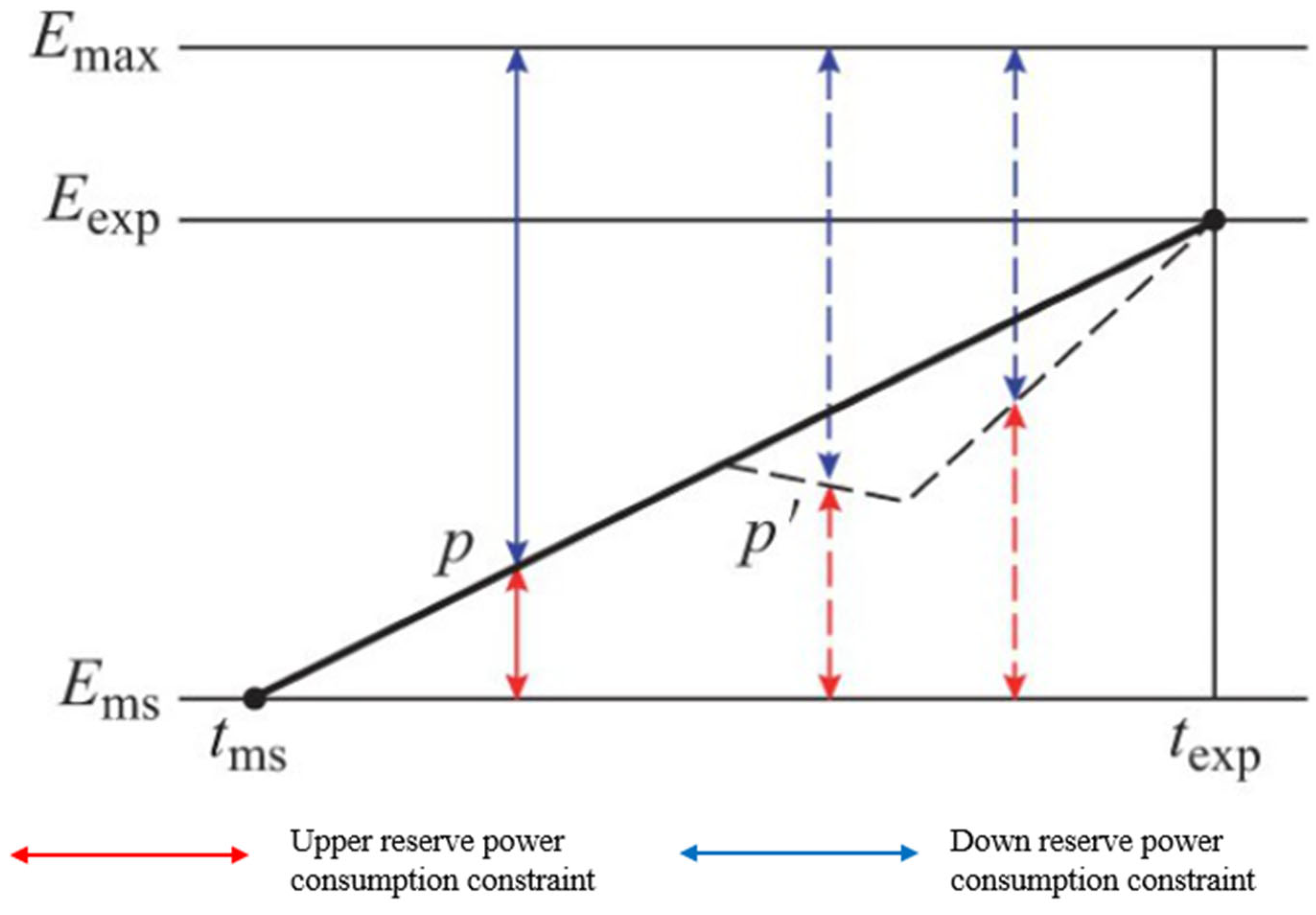
Electricity boundary is represented by maximum/minimum electricity quantity, and the boundary is in dynamic change at each time, and the change in a previous dispatching process will also cause the change in the subsequent electricity quantity boundary. It is the existence of the electricity quantity boundary that ensures that the dispatching of EV does not breach the contract; however, due to the change in power boundary caused by this, the adjustable ability of EV is more limited than that of traditional units, which is mainly reflected in the fact that it cannot continuously provide peak regulation or reserve capacity for a long time. Figure A1 shows the change in battery power corresponding to charging/discharging power operation. Before the power reaches the guaranteed power, the EV temporarily loses its controllability, and when the guaranteed power is reached, the power boundary affects the EV reserve energy as follows:
E ( t ) = E s t a r t + P L , max ( t t s t a r t ) , t t m s E m s E ( t ) E max , t m s t t exp
E ( t exp ) E exp
E ( t ) = E s t a r t + t s t a r t t P ( t ) d t
where E ( t ) is the real-time battery charge. Due to the power boundary effect, to ensure that the desired power requirement of the user is met within the scheduled time, the EV is not regulated until the start of the regulation period, and then it goes off grid ( t m s ~ t exp ), all with minimum power requirements:
E min ( t ) = E m s , t m s t t exp E exp E m s P L , max E exp P L , max ( t exp t ) , t exp E exp E m s P L , max t t exp
Equation (26) can, therefore, be expressed as follows:
E ( t ) = E s t a r t + P L , max ( t t s t a r t ) E min ( t ) E ( t ) E max
In addition to the power and quantity boundaries, considering the protection of battery life [57], the contract also includes conditions such as discharge depth D and discharge number n c that limit the discharge process, which will essentially reduce the charge/discharge path of the EV within the feasible range. For the formalization of these two constraints, the discharge depth constraint can be formalized by replacing Ems in Formula (29) with Formula (31); if the discharge number constraint is considered to be at most one in a single scheduling period, the form is shown in Equation (32).
E m s = max ( E m s , ( 1 D ) E max )
n c 1
By discretizing Equation (28), a more general formula for calculating EV capacity can be obtained as follows:
E ( k ) = E s t a r t + υ ( k ) k = 1 n P ( k ) Δ t
where υ ( k ) indicates whether the EVs are grid-connected or not. Therefore, by combining Equations (22) to (33), the spare capacity of EVs can finally be obtained, and the upper and lower spare capacity boundaries of EV clusters can be subsequently obtained by Minkowski aggregation.
R c u p = P c u ( k ) = υ ( k ) max ( min ( P G , max + P ( k ) , E ( k ) E min ( k + 1 ) Δ t + P ( k ) ) , 0 )
R c d o w n = P c d ( k ) = υ ( k ) max ( min ( P L , max P ( k ) , E max E ( k ) Δ t P ( k ) ) , 0 )

2.2. MRMR Algorithm Considering Causality

The conditioning bounds for distributed reserve resources can be obtained by performing Minkowski aggregation of the various distributed resource clusters in Section 3.1 [58]. To extract the mapping relationship between numerical weather prediction (NWP) data and the regulation boundaries of distributed reserve resources, it is essential to clarify both the correlation and causality between various meteorological features and the reserve capacity limits. NWP data often contain a large number of highly similar variables—such as wind speeds at 10 m, 30 m, and 50 m heights—which may introduce excessive redundancy and hinder the model’s ability to effectively capture the relationship between inputs and target labels. Therefore, this study employs a mutual information-based mRMR algorithm to identify an optimal subset of features. A secondary screening is then conducted using Granger causality tests to ensure the selected features possess both statistical relevance and physical interpretability. The complete algorithmic procedure is presented in Appendix A. In the following section, we introduce the core concepts of the method, beginning with the definition of mutual information.
I ( x , y ) = p ( x , y ) log 2 p ( x , y ) p ( x ) p ( y ) d x d y
where x denotes the characteristic variable, y denotes the target variable. p ( x , y ) is the joint probability density function; p ( x ) together with p ( y ) are the edge probability density functions, respectively.
Assume the set of all features x is denoted as F , of which x = { x 1 , x 2 , x n } , n is the number of features. We aim to first select the subset S m consisting of the top m most relevant features, which should satisfy the following relation:
max D ( S m , y ) D = 1 m x i S m I ( x i ; y )
By means of Equation (37), we obtain a collection of features S m , which has the largest average mutual information value between the features in the set and the target variable. However, in order to achieve the goal of minimizing redundancy, there is a possibility of large redundancy between the features in S m ; so S m needs to be further satisfied:
f 1 = min R ( S m ) R = 1 m 2 x i , x j S m I ( x i ; x j )
The resulting subset of features S m should satisfy the following maximum relevance–minimum redundancy principle:
f 2 = max Φ ( D , R ) Φ = D R
Through the incremental search algorithm, if we have already selected the m 1 features and formed a subset of features S m 1 , then it is possible to extract from the remaining features the m-th feature. The following needs to be satisfied:
f 3 = max x j F S m 1 ( I ( x j ; y ) 1 m 1 x i S m 1 I ( x j ; x i ) )
For the preliminarily selected feature subset S m , the Granger causality test can be applied to further verify whether a given feature x contributes to the prediction of the target variable y . The principle of Granger causality is defined as follows: if the past information of both the feature x and the target variable y improves the prediction of y , compared to using only the past information of y , then x is said to help explain the future variation of y , and x is considered a Granger cause of y .
After selecting each feature x and the target variable y , a stationarity test is performed on the data. Multi-order differencing is applied to non-stationary series to achieve stationarity. Based on the stationary series, the Bayesian Information Criterion is used to determine the optimal lag order, and a Vector Autoregression (VAR) model is established to characterize the temporal relationships among the variables. The fitted VAR model is expressed as follows:
y t = a + v = 1 u β v x t v + v = 1 u γ v y t v + ε t
where a is a constant term. β v , γ v are the regression coefficient. u is the maximum lag order; ε t is the residual term. The original hypothesis was β v = 0 . The fitted model was then used for Granger causality test. The test statistic is the covariance matrix based on the residuals, which is tested using the F-statistic; the larger the F-statistic, the more significant the effect of the independent variable on the target variable is. Judgement was made based on the results of the Granger causality test. If the p-value is less than the set level of significance, the original hypothesis is rejected, and the independent variable is considered to have a significant effect on the target variable. Otherwise, the original hypothesis is accepted, and no causal relationship is considered. After eliminating the features with no causal relationship, a subset of features can be formed after the second screening S m .

2.3. Adaptive Integrated Learning Framework Considering Model Diversity

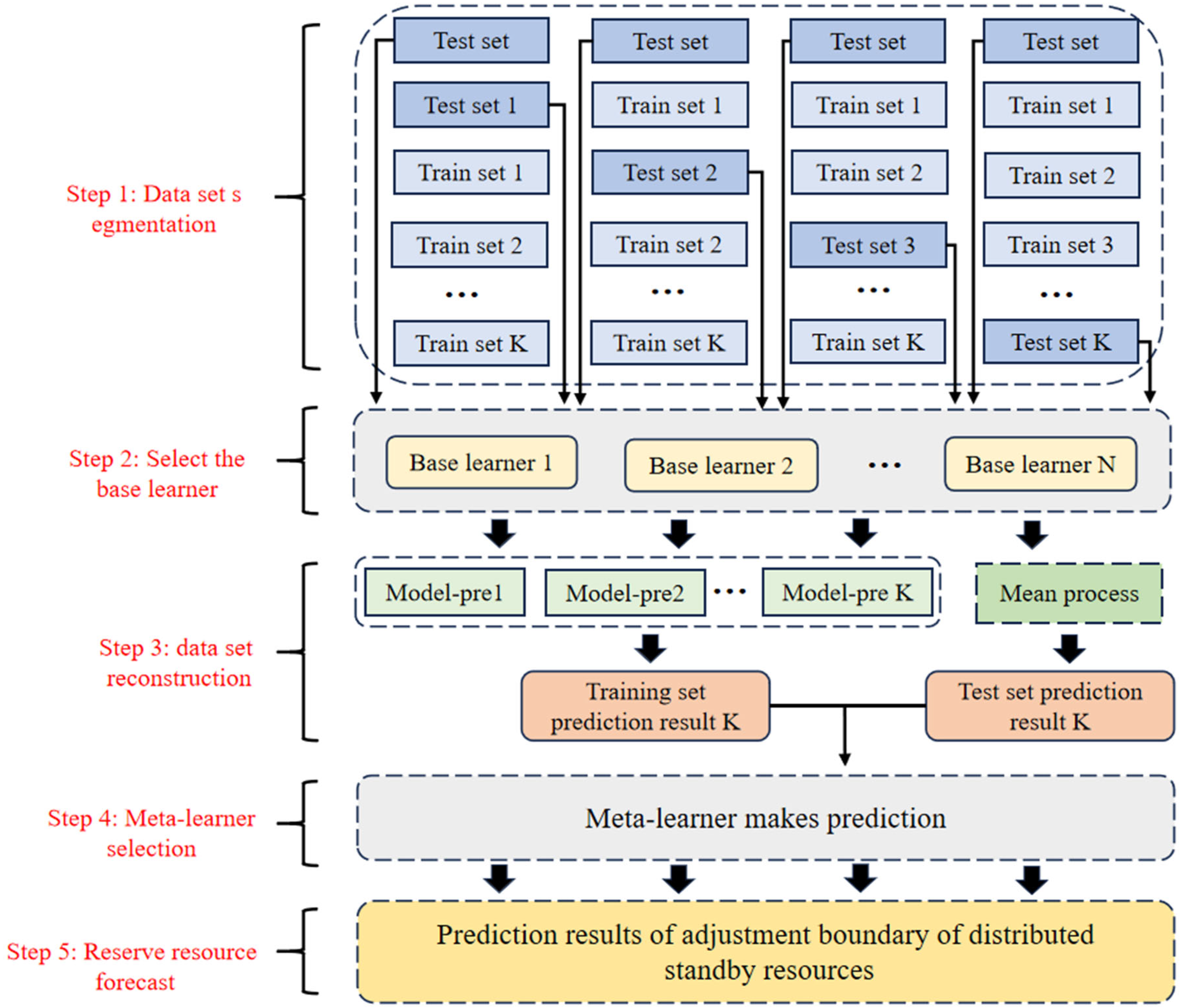
The paper develops a response capability evaluation model for distributed reserve resources based on the stacking algorithm. Unlike Bagging and Boosting, which integrate multiple learners of the same type, the stacking model combines different types of base learners in a single stack to achieve superior performance that cannot be attained by any individual learning algorithm alone. The specific model framework is shown in Figure 2.
In order to improve the prediction performance of the model and reduce the risk of overfitting, this study adopts the stacking integrated learning method based on K-fold cross-validation. The method combines the prediction results of multiple base learners in a hierarchical manner and further corrects the prediction errors with the help of a meta learner, so as to improve the generalization ability and robustness of the overall model. The following describes the training process. Firstly, the original dataset S is randomly divided into K equal number of subdatasets S 1 , S 2 , S k as a basis for cross-validation. Then, for each base learner i , the K-fold cross-validation method was used: one of the subsets S k was selected each time as the validation set and the remaining K 1 subsets as the training set to train the K sub-models and obtain the predictions of this learner for all samples. These K predictions from the sub-validation are stitched together into a complete prediction output D i , whose sample size is consistent with that of the original dataset. For all n repeating the above process for each base learner, we can obtain n predictive outcome datasets D 1 , D 2 , D n . They are spliced by columns to form a new feature dataset D = [ D 1 , D 2 , D n ] as the input to the second layer of the meta learner, while its corresponding labels are still the original set of labels S . Finally, the meta learner is trained to learn the relationship between the base learner output and the real labels. Since the meta learner is constructed on the basis of the base learner prediction, it is able to model the systematic deviation and local error in the first layer model twice, so as to improve the accuracy and generalization performance of the overall model. Evidently, different types of models have their own advantages in terms of modelling structure, nonlinear fitting ability, and generalization performance. In order to enhance the diversity and robustness of the integrated models, 14 representative models, including tree models, kernel methods, neural networks, and Bayesian methods, are selected as the alternative base learners of the stacking framework. The meta learners are finally identified as ridge regression through the experimental results.

3. Case Study

3.1. Experiment Details and Settings

This section describes the dataset, evaluation metrics, and hardware details used for the model. The experimental hardware configuration for this study is a 2.4 GHz Intel® Core™ i5-10200H (8-core) CPU equipped with 16.00 GB of RAM and implemented in the Python (3.8) language based on the PyTorch (2.0) framework under the Windows 11 operating system. For the NWP data and wind PV power data, the dataset released by the State Grid is selected [59]. The time scale of this dataset is from 2019 to 2020, and the granularity of the data is 15 min. In this paper, the NWP data are mapped to 1 h by averaging, and the new energy output data are mapped to 1 h by summing. For the distributed energy storage, EV, and load side data, Monte Carlo simulation is used to simulate the parameters, and the economic self-scheduling model is used to obtain the reserve capacity of each type of distributed resource. The tariff data and related simulation parameters are shown in Appendix B. In addition, the modelling of distributed reserve capacity is essentially a time series prediction problem, so the evaluation indexes used in this paper mainly include five indexes, namely, RMSE, MSE, MIAE, MAPE, and R2, and the ratio of the training set, the validation set, and the test set is 8:1:1.
R M S E = 1 n i = 1 n ( Y i Y ^ i ) 2
M S E = 1 n i = 1 n ( Y i Y ^ i ) 2
M A E = 1 n i = 1 n ( Y i Y ^ i )
M A P E = 100 % n i = 1 n Y ^ Y i Y i
R 2 = 1 i = 1 n ( Y i Y ^ i ) 2 i = 1 n ( Y i Y ¯ i ) 2
Among them, the smaller the values of RMSE, MSE, MAE, and MAPE are, the better the model fitting effect is; the value of R2 ranges from 0 to 1, and the closer to 1, the better the model fitting effect is.

3.2. Spare Capacity Generation and Feature Selection

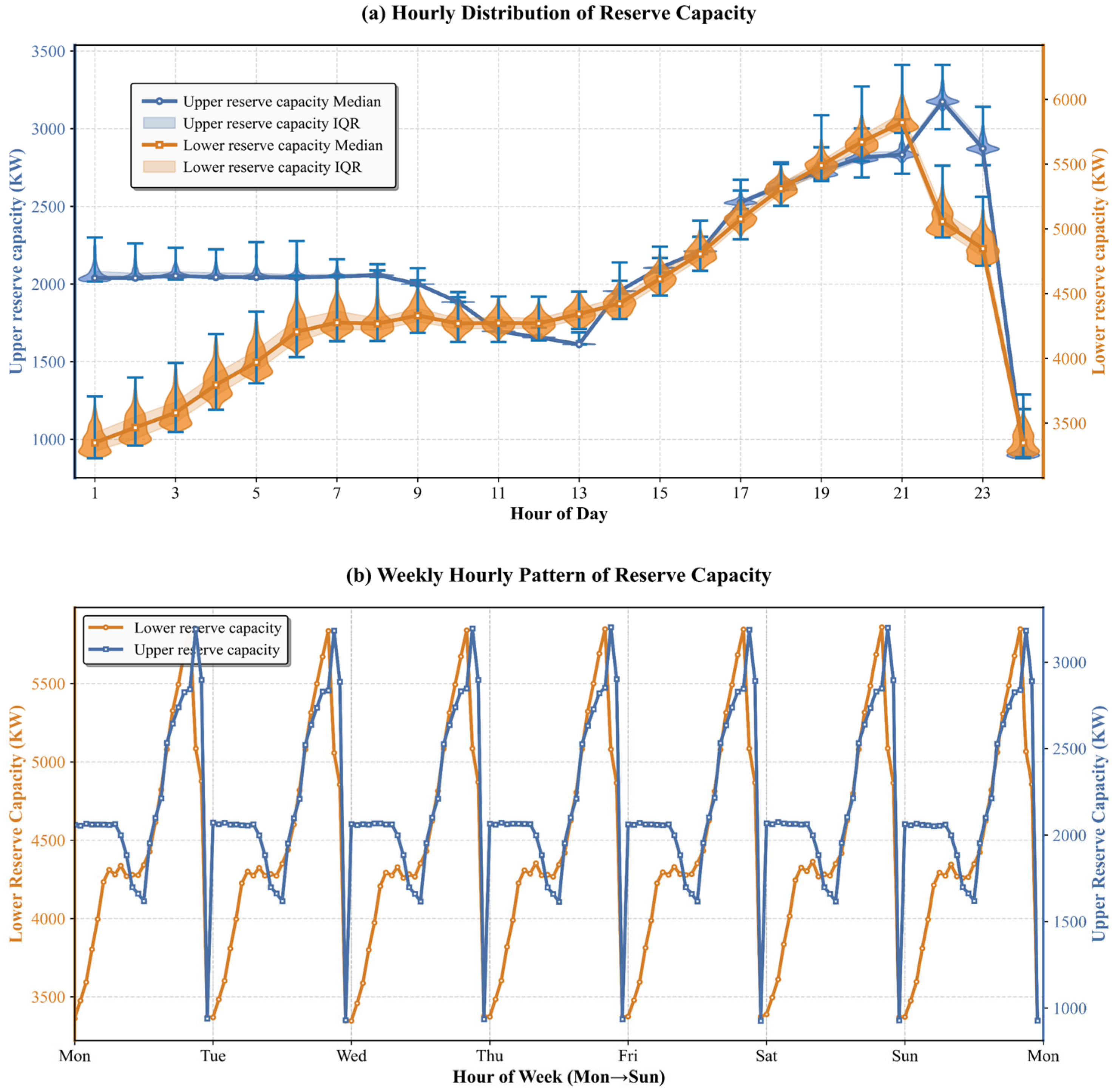
This study evaluates the upper and lower spare capacities provided by distributed resources in the sample period by aggregating the spare capacities of multiple types of distributed resources and further analyses their statistical distribution and change patterns on the intra-day and intra-week scales. Figure 3 presents the typical time-sequence characteristics of the spare capacities and systematically reveals the dynamic change trends of the capacities of distributed spare resources. In terms of intra-day distribution, the upper spare capacity provided by distributed resources is at a lower level from 0:00 to 14:00, with smaller fluctuation; it rises significantly from 15:00 to 22:00, and reaches a peak around 21:00, which indicates that it has stronger upward adjustment capacity in the evening and helps to cope with the system flexibility demand during the evening peak. In contrast, the downside reserve capacity remains high throughout the day, showing a tendency to increase over time, especially during the high daytime load period, reflecting the good load shedding ability and down-regulation potential of distributed resources. On the intra-weekly scale, the reserve capacity shows an obvious daily cycle pattern. Both weekday and weekend reserve capacities show a consistent pattern, i.e., a trough at night and a gradual rise to a peak during the day, reflecting a high degree of repeatability and predictability. Although there are slight differences in the reserve capacity values of different day types, the overall fluctuation trend remains consistent, and this regular time-sequence change is likely to be closely related to the structural characteristics of the PV and wind power generation capacity as well as the behaviour of the energy-using loads in the time dimension. In summary, the distributed reserve resources show significant periodicity and regularity in the time scale, which not only provides data support for understanding their regulation potential but also lays a good foundation for subsequent reserve capacity prediction based on machine learning or time series modelling. The existence of periodicity significantly enhances the feasibility and accuracy of reserve capacity prediction and provides a strong support for the active participation of distributed resources in auxiliary services.
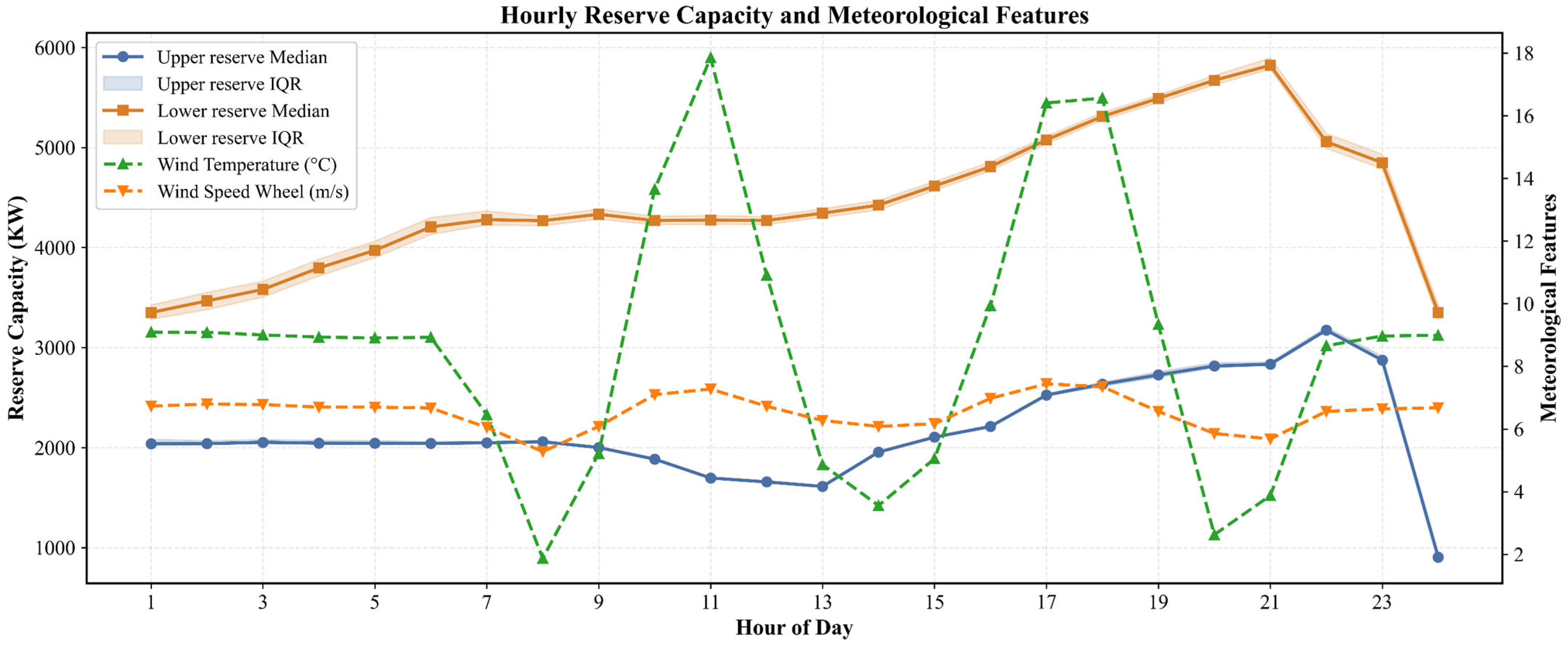
To improve prediction accuracy and efficiency, and after confirming that the distributed reserve capacity is predictable, this study applies the mRMR algorithm—considering causality—to screen meteorological features. The results are presented in Table 2. The mutual information values in the table represent the average mutual information between each meteorological factor in the NWP dataset and the upward and downward reserve capacities. All features are ranked under the principle of minimizing redundancy among them. The p-values and F-values correspond to the results of Granger causality tests between each meteorological factor and the upward and downward reserve capacities, respectively. Among the nine meteorological variables, only direct irradiance and global irradiance fail to pass the test. The remaining seven variables pass the causality test, at least at the 10% significance level, and are selected as the optimal feature subset. To further illustrate the temporal patterns and relationships between the selected features and reserve capacity, Figure A5 presents the hourly distribution of the upward and downward reserve capacities alongside two representative meteorological features: Wind_temperature and WindSpeed_wheel. This visualization allows readers to observe peaks, trends, and fluctuations in both reserve capacities and meteorological variables, providing an intuitive interpretation of the feature–reserve relationship and complementing the results with mutual information and Granger causality analysis.

3.3. Model Parameter Setting and Difference Analysis

In order to optimize the performance of stacking, it is necessary to analyze the learning ability and variability of each learner. Table 3 shows the parameter settings of 14 meta learners, covering tree models, machine learning, Bayesian methods, and deep learning model structures.
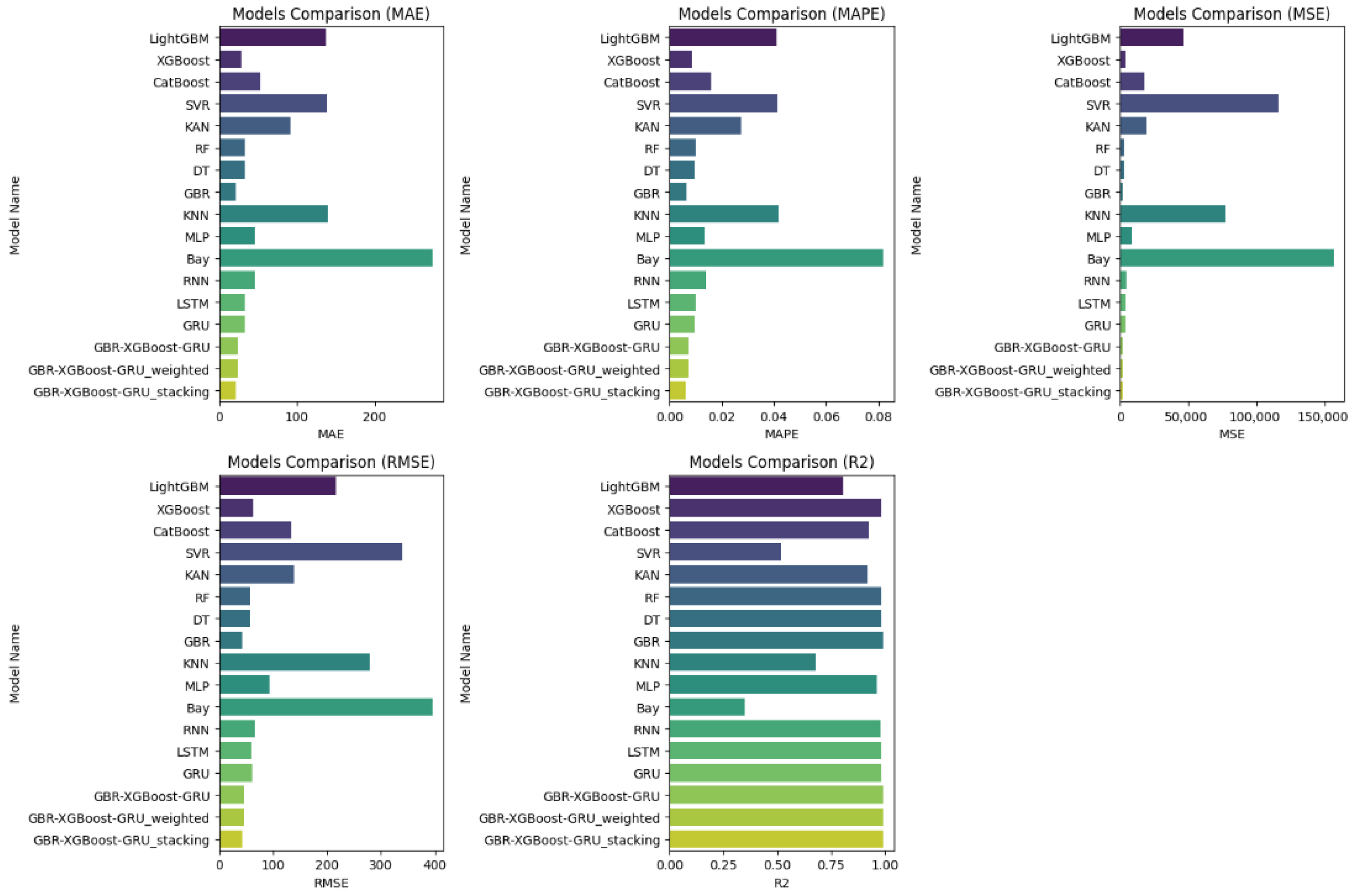
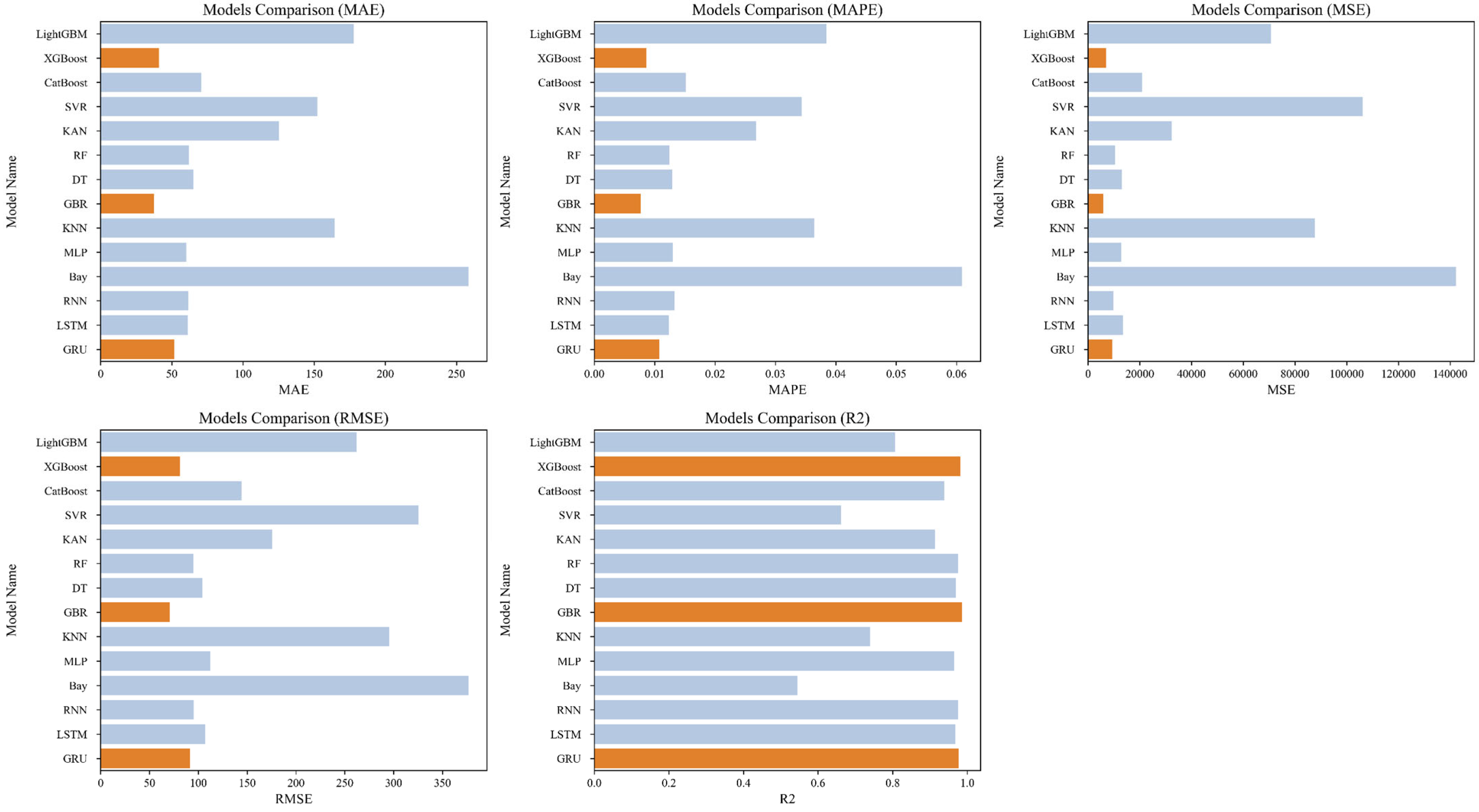
Figure 4 presents the average upper- and lower-reserve prediction results for each candidate base learner. In terms of overall prediction accuracy, GBR, XGBoost, and GRU consistently outperform the other models across most evaluation metrics. Specifically, they achieve significantly lower errors in MAE, RMSE, and MAPE, while R2 values are close to 1, demonstrating strong fitting ability and generalization performance in capturing the nonlinear variations in reserve capacity.
Among these models, XGBoost and GBR, as ensemble tree-based models, excel in feature selection and nonlinear modelling, effectively capturing periodic and fluctuating patterns inherent in reserve capacity data. GRU, a variant of recurrent neural networks, benefits from its gating mechanism, which enables it to capture both short- and long-term dependencies in time series, showing stable performance in modelling intra-day and intra-week temporal dynamics. In contrast, simpler models, such as a single decision tree (DT), KNN, or Bayesian regression, perform poorly across multiple metrics, highlighting their limited ability to model high-dimensional nonlinear relationships and temporal structures. Although deep neural networks (e.g., MLP, LSTM, RNN) perform well on some metrics, they are sensitive to hyperparameter settings and exhibit slightly lower model stability.
To ensure fair comparability among models, we initially set uniform parameters for all candidates and selected several base learners based on performance. Furthermore, we applied Bayesian hyperparameter optimization to all candidate models, as shown in Figure A4. The results indicate that the optimal base learners remain unchanged, confirming their suitability for use as base learners in the stacking ensemble.

3.4. Prediction Result Analysis

3.4.1. Reserve Capacity of Typical Scenes in Four Seasons

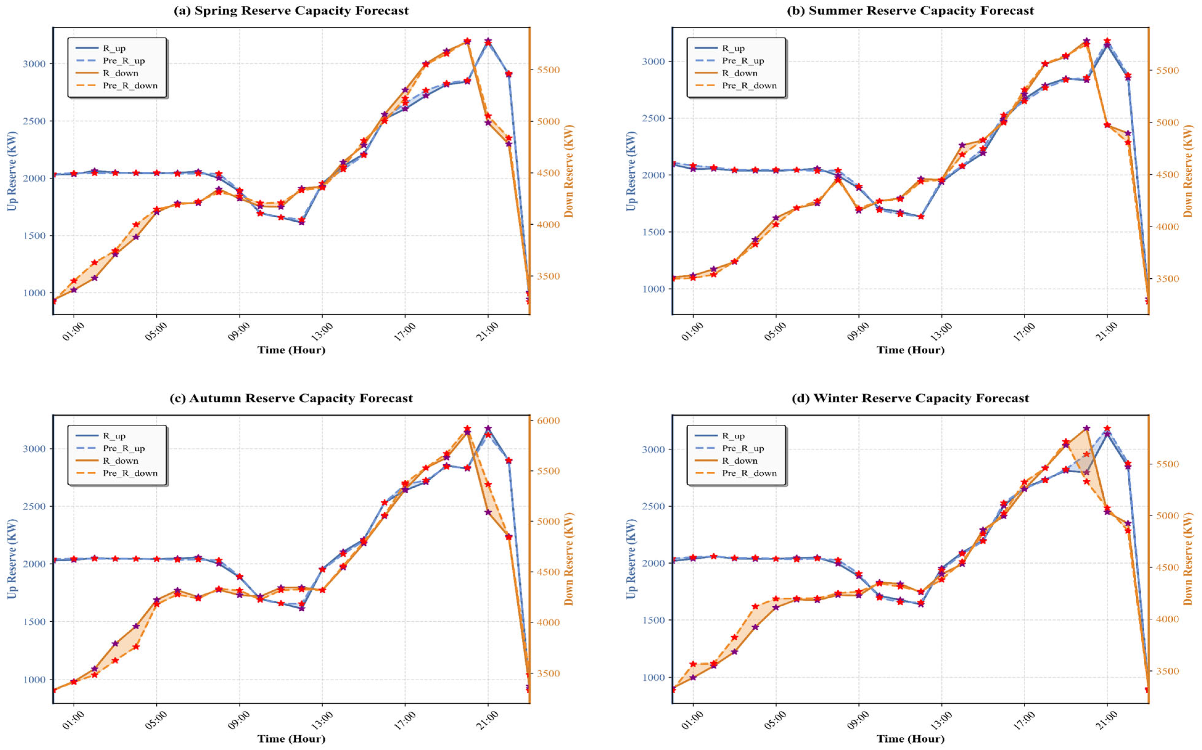
In order to show the effectiveness of the constructed stacking model, the study selects the typical days of spring, summer, autumn, and winter seasons in the dataset to show the results of the upper- and lower-reserve prediction, the specific results are shown in Figure 5. From the overall trend analysis in the figure, it can be seen that the reserve capacity of the four seasons shows obvious time characteristics: the reserve capacity demand is lower in the early morning hours and gradually rises in the morning hours, peaks between 17:00 and 20:00, and then rapidly declines. This pattern of change is closely related to the peak and valley cycles of power loads, indicating that the allocation of spare capacity is significantly driven by power load fluctuations; specifically, the upper- and lower-reserve capacity peaks are higher in summer and winter than in spring and autumn, which is closely related to the significant increase in air-conditioning and heating loads under extreme temperature conditions. In these high-load scenarios, there is also more spare capacity required to ensure system stability. In addition, the change in reserve capacity is relatively smooth in spring and autumn, especially in spring, when the difference between daytime and nighttime loads is small, resulting in little change in the reserve capacity curve. From the perspective of prediction accuracy, the predicted results in the four subplots fit well with the actual values, indicating that the model can capture the dynamics of reserve capacity in different seasons more accurately. The upper- and lower-reserve forecast curves in summer and autumn almost coincide with the actual curves, showing high accuracy; while the forecasts in winter are slightly lower than the actual ones, which may be due to the effect of the lag in the model’s response to the extreme weather conditions, and it is necessary to reduce the model’s sensitivity to the forecast of the reserve capacity under the extreme weather conditions in the future.

3.4.2. Prediction Performance of the Model Under Extreme Climate

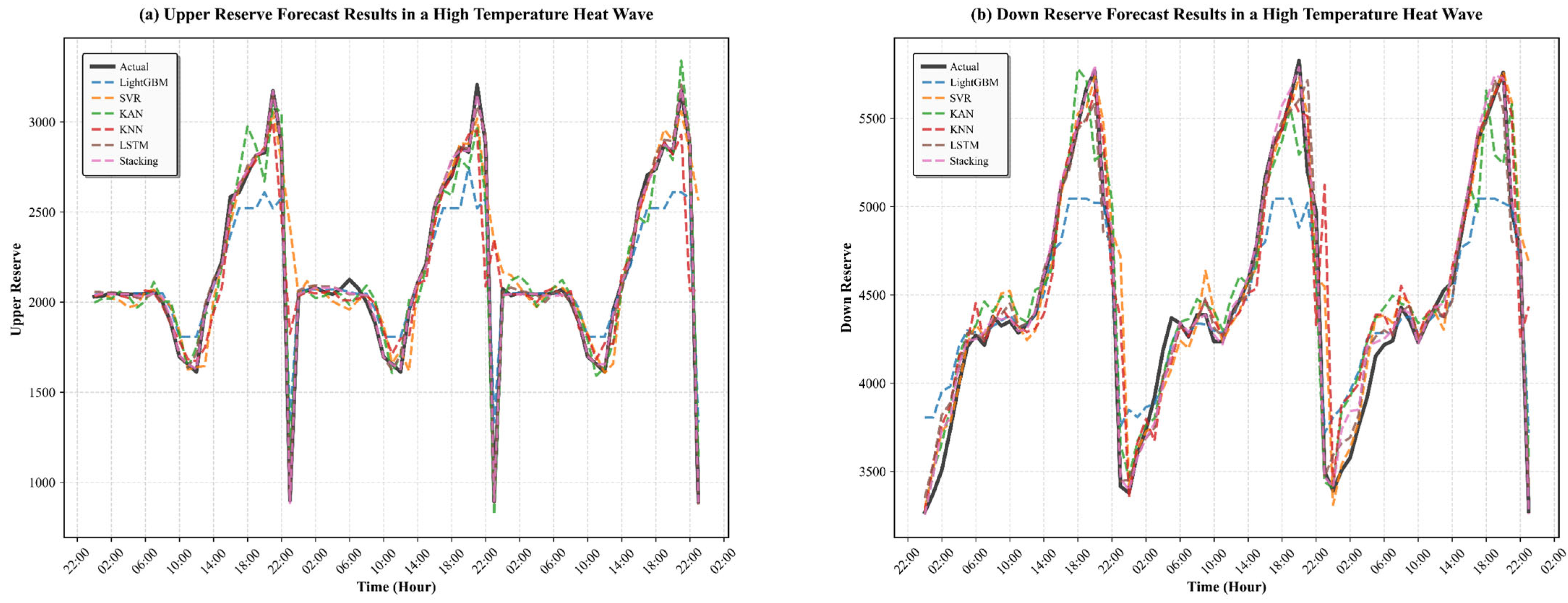
In order to further illustrate the applicability and robustness of the constructed stacking model under the influence of extreme weather, this study selects high-temperature heatwave and windy weather as cases and compares and analyses the prediction results with kernel methods, tree models, deep learning models, etc. Figure 6 shows the prediction effect of reserve resources under high-temperature heatwave weather. High-temperature heatwave refers to an extreme weather process in which the daily maximum temperature reaches or exceeds 35 °C for three or more consecutive days, which is usually accompanied by meteorological features such as high radiation, low wind speed, and high humidity. Driven by high temperatures, the upper- and lower-reserve capacities show obvious intra-day cyclical peaks, especially during the mid-day to evening periods with sharp fluctuations. Most of the models are able to capture the basic trend of reserve capacity well, but there are still some deviations at the peaks. Among them, KNN and LightGBM show overestimation or lagging in the extreme value interval, which indicates that they are not responsive to sudden load changes. In contrast, KAN, LSTM, and stacking model perform better in time series modelling and nonlinear fitting, and can more accurately restore the rapid change process of the upper- and lower-reserves under high temperature, especially the stacking model, which improves the robustness and generalization ability of load fluctuation under the mechanism of multi-model fusion and is more adaptable.
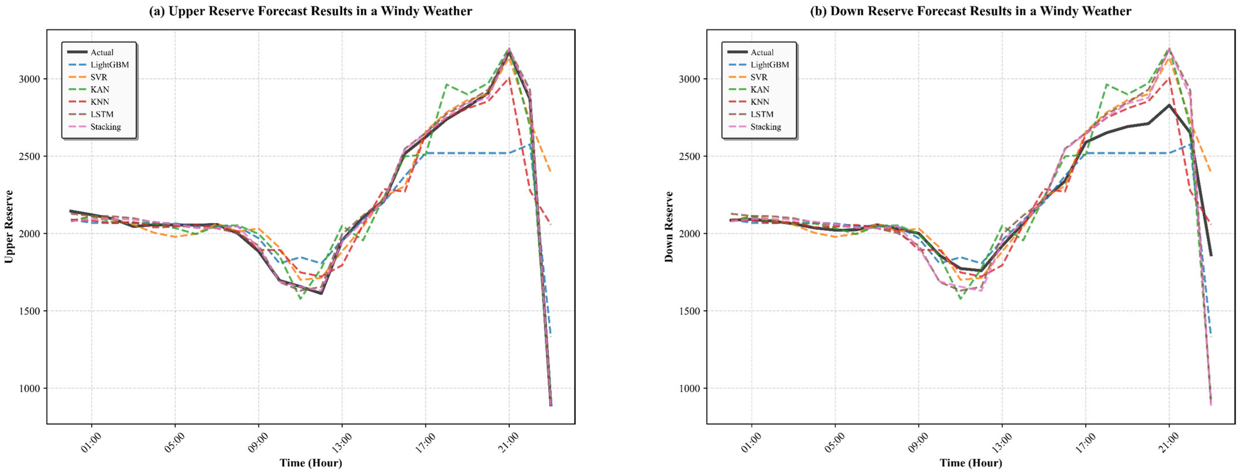
Compared with the drastic fluctuation in reserve demand caused by high loads in a heatwave, the trend of reserve capacity change in windy weather is relatively smooth, and the prediction difficulty is reduced accordingly. Figure 7 shows the up and down reserve prediction results under typical windy weather scenarios. Under the influence of strong wind, the fluctuation in wind power output increases significantly, which poses a challenge to the system’s ability to regulate resource scheduling. Overall, the fitting results of the models in the windy scenario are generally better than those in the high-temperature and heatwave scenarios, especially in the low and medium fluctuation ranges of the reserve capacity, and almost all of the models are able to track the real curves well. Compared with the aforementioned high-temperature scenario, the stacking model also shows strong prediction ability in the windy scenario, especially in the stage of rapid increase and decrease in reserve capacity, and its error is significantly smaller than that of a single model; in addition, the SVR and LSTM also show better performance, which indicates that they are adaptable to deal with nonlinear fluctuations caused by the wind speed. However, KNN, and LightGBM still have some lags and deviations at the peak, indicating that their ability to respond to the reserve demand triggered by the sudden change in wind speed is still limited.

3.4.3. Compared with Single Model and Benchmark Strategy

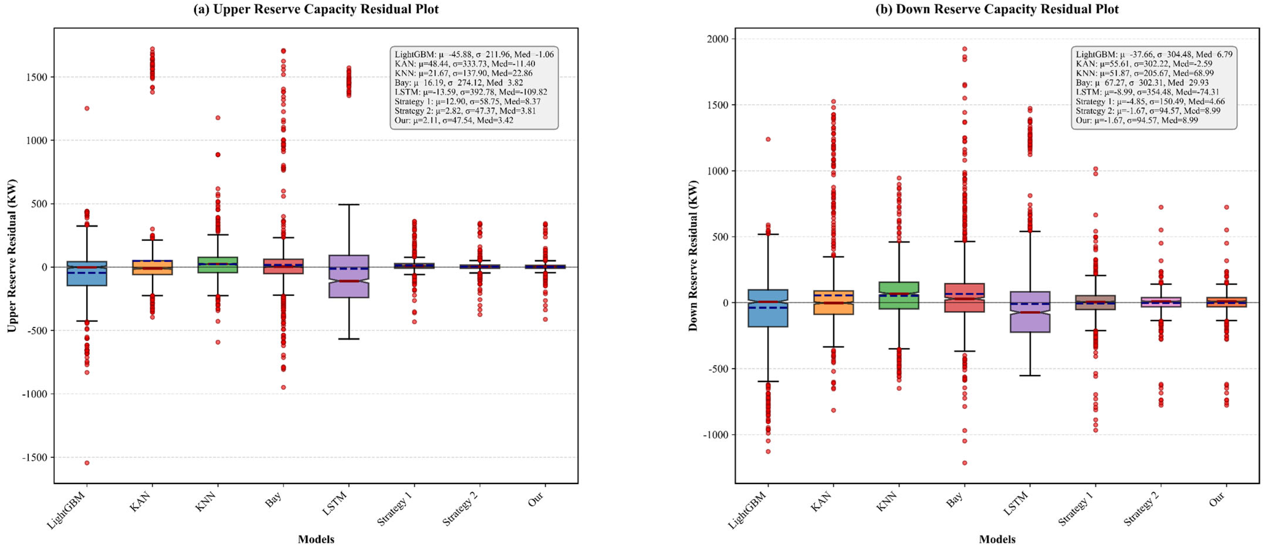
The meta learner for the stacking model constructed in this study is ridge regression. In order to verify the reasonableness of this framework, we compare its prediction results with a single model on a test set. In addition, two other integration strategies are designed in this paper, Strategy 1 is averaging the prediction results of the three base learners, and Strategy 2 is weighting the prediction results of the three base learners according to the value of MAE. Figure 8 shows the prediction errors of each model and strategy. From the distribution of the residuals of the upper spare capacity, the residuals of the stacking method are mainly concentrated in a small range of values, and the height of the box is relatively small, which indicates that the prediction accuracy is higher and the volatility is smaller. In contrast, the residual distributions of other single models have a wider range and more outliers. The residual distribution of the lower spare capacity further verifies this conclusion, and the median of the stacking method is closer to zero and the interquartile range is smaller, indicating that the prediction bias is effectively controlled. Compared with the simple average integration of Strategy 1, the stacking method is able to adaptively learn the weight assignment of each base learner, avoiding the performance loss that may be brought by equal weights. Compared with the weighted integration based on the inverse of MAE in Strategy 2, the stacking method can better capture the complex relationship between base learners through ridge regression meta-learning and achieve a more accurate fusion of prediction results.

3.4.4. Compared with Other Mixed Models

To provide a clearer interpretation of the numerical results in Table 4 and Table 5, this section explicitly compares the performance of the proposed stacking model with the six conventional hybrid models across all evaluation metrics. For the upper-reserve prediction (Table 4), the stacking model achieves an R2 of 0.996, which is comparable to the best-performing hybrid models (e.g., CNN-BiLSTM and CNN-BiGRU with R2 = 0.997), while its MAE and RMSE remain within a competitive range. Importantly, the computational time of the stacking model (130.85 s) is substantially shorter than that of deep hybrid models, most of which require 500–800 s to complete training. A similar pattern is observed for the lower-reserve prediction (Table 5): the stacking model attains an R2 of 0.991, close to the optimal values of the neural network-based models but with a significantly lower training time of 133.71 s. These results clearly indicate that although several neural network hybrids achieve marginally lower error metrics, they do so at the cost of very high computational expenses. In contrast, the proposed stacking framework achieves an effective balance between accuracy and efficiency, offering near-optimal predictive performance while reducing training time by a wide margin compared with the deep hybrid baselines. This makes the stacking model particularly suitable for operational environments requiring fast response and frequent retraining.

4. Conclusions and Future Works

4.1. Conclusions

In this paper, we sort out multiple types of distributed resources on the generation, load, and energy storage sides, construct an economic self-scheduling model integrating meteorological uncertainty, and use Minkowski and aggregation methods to uniformly draw the reserve capacity boundary of resource clusters; then, combining the principle of mRMR and Granger causality test, we downscale the high-dimensional meteorological features to enhance the model modelling efficiency and physical interpretation; finally, we construct an end-to-end integrated learning framework based on stacking to achieve efficient prediction from multi-source meteorological features to reserve capacity. Finally, an end-to-end integrated learning framework based on stacking is constructed to achieve efficient prediction from multi-source meteorological features to backup capacity. The conclusions of the study are as follows:
(1)
Temporal characteristics and feature interpretability enable efficient modelling. Distributed reserve capacity on the generation, load, and storage sides exhibits clear diurnal and weekly patterns, providing a stable foundation for predictive modelling. By combining mRMR with multi-stage Granger causality screening, the framework extracts key meteorological drivers and removes redundant variables, substantially enhancing training efficiency and preserving physical interpretability.
(2)
The stacking model achieves a superior balance between accuracy and computational efficiency. Across upper- and lower-reserve prediction tasks, the proposed integrated model attains an average R2 of 0.994. Meanwhile, its training times (130.85 s and 133.71 s) are significantly lower than those of conventional neural or hybrid models, demonstrating clear advantages in generalization, scalability, and overall computational performance.
(3)
High robustness under extreme weather and clear superiority over other ensemble strategies. The model maintains stable error indices under extreme meteorological conditions such as heatwaves and strong-wind events, accurately capturing multi-peak reserve responses. Comparative experiments further show that the stacking strategy consistently outperforms simple averaging and MAE-weighted integration across all evaluation metrics, confirming its effectiveness as the optimal ensemble scheme.

4.2. Future Works

Although this paper has conducted a systematic study on predicting the reserve capacity of multi-type distributed resources, several limitations remain that warrant further investigation. At the feature engineering level, our work currently focuses on screening the optimal subset of meteorological features but has not explored combinatorial or composite feature relationships, and future work could introduce operator-based construction methods to generate richer composite features with stronger expressive power. At the model training level, the current end-to-end integrated learning model is trained offline in a static manner, limiting its adaptability to dynamic changes in the operating environment, and future research will explore online and real-time learning frameworks that dynamically adjust model parameters as new data arrives. At the level of practical engineering applications, the present approach predicts distributed reserve capacity but does not form a closed loop with scheduling optimization, and subsequent work will aim to develop integrated prediction–decision frameworks to improve coordination and practicality. In addition, future studies will integrate uncertainty quantification to provide probabilistic reserve forecasts, expand validation using diverse datasets from different geographic regions and climates, explore transfer learning to leverage knowledge from related energy systems and enhance generalization, employ synthetic data augmentation to improve robustness against rare extreme meteorological events, and optimize computational efficiency to enable deployment in real-time power system operations. These directions are expected to enhance the model’s adaptability, robustness, and practical value in real-world distributed energy systems.

Author Contributions

Conceptualization, C.G. and P.Y.; methodology, Z.C.; software, Y.C.; validation, Y.C.; formal analysis, F.K.; investigation, B.W.; resources, B.W.; data curation, B.W.; writing—original draft preparation, Z.C.; writing—review and editing, P.Y.; visualization, Z.C.; supervision, C.G.; project administration, C.G.; funding acquisition, P.Y. All authors have read and agreed to the published version of the manuscript.

Funding

This research was funded by the Science and Technology Project of China Southern Power Grid, grant number 030000KC24090071.

Data Availability Statement

The original contributions presented in this study are included in the article. Further inquiries can be directed to the corresponding authors.

Acknowledgments

Thanks to the editorial department and anonymous reviewers for their hard work.

Conflicts of Interest

Authors Chao Gao, Bin Wei, Yabin Chen and Fan Kuang were employed by Guangdong Power Grid Co., Ltd. The remaining authors declare that the research was conducted in the absence of any commercial or financial relationships that could be construed as a potential conflict of interest.

Abbreviations

LightGBMLight Gradient Boosting Machine
XGBoosteXtreme Gradient Boosting
CatBoostCategorical Boosting
SVRSupport Vector Regression
KANKolmogorov–Arnold Networks
RFRandom Forest
DTDecision Tree
GBRGradient Boosting Regressor
KNNK-Nearest Neighbours
MLPMulti-Layer Perceptron
BayBayesian Ridge
RNNRecurrent Neural Network
LSTMLong Short-Term Memory
GRUGated Recurrent Unit
Temp_centerCentral temperature of membership function
Temp_stdStandard deviation of normal distribution in each temperature zone
Temp_weightInfluence weight of each temperature zone on access intention
TemperatureActual ambient temperature
T b a s e User-set comfort temperature
Δ T Comfortable temperature tolerance intervals
κ Heat conduction efficiency
δ Refrigeration rate
P r i c e t h r e s h o l d Electricity price-response threshold
T i n d o o r User indoor temperature
T o u t Outdoor temperature
P r a t e d Maximum operating power of a single air conditioner
γ ¯ Maximum response rate
N max Maximum daily continuous adjustment time
Ω Total duration of maximum response per day
P r a t e d Maximum operating power of a single water heater
P total Daily hot water energy consumption
P ¯ Maximum increased load in a single period
P _ Maximum load reduction in a single period
η s h i f t Initial hot water energy storage state
E max Battery capacity
S O C s t a r t Initial state of charge
t s t a r t Access time of electric vehicle
P G , max Maximum discharge power
P L , max Maximum charging power
S O C exp Expected final SOC
S O C m s Guaranteed SOC limit
S O C i n i t Rated capacity of energy storage unit
S O C m a x Maximum SOC
S O C m i n Minimum SOC
P ¯ c Maximum charging power
P ¯ d Maximum discharge power
η c Energy storage charging efficiency
η d Energy storage discharge efficiency

Appendix A

Algorithm A1 shows the pseudo-code of the feature screening algorithm designed in this study. The algorithm firstly evaluates the correlation between features and target variables through mutual information and minimizes redundancy among features while maintaining high correlation. Subsequently, a Granger causality test is performed on the initial set of features to further eliminate redundant variables that are not causal and finally form a subset of features with more explanatory and predictive power.
Algorithm A1 Feature Selection Algorithm Based on Maximum Correlation-Minimum Redundancy and Causality Screening
Input: Feature set F = { f 1 , f 2 , f n } , Target variable y , Required feature number k Significance level α .
Output: Optimal feature subset S f i n a l after final screening.
1.
Initialize the selected feature set S , the candidate feature set R F .
2.
Calculate the mutual information between each feature f i F and the target variable y : M I ( f i , y ) = p ( f i , y ) log 2 p ( f i , y ) p ( f i ) p ( y ) d f i d y .
3.
Select an item f * with the greatest mutual information with y to add to S and remove it from R : f * = arg max f i R   M I ( f i , y ) .
4.
for t = 2 , 3 , 4 , k do:
5.
For each f j R , calculate its redundancy: Re d ( f j ) = 1 S f s S M I ( f j , f s ) .
6.
Calculate the comprehensive score: S c o r e ( f j ) = M I ( f j , y ) Re d ( f j ) .
7.
Select the f * with the highest score to join S and remove it from R .
8.
end for
9.
V A R model is constructed for each feature f i , and y in S , and Granger causality test is caried out.
10.
If p value is less than α , keep f ; Otherwise, it is eliminated from S .
11.
Let the final feature subset S f i n a l = S .
12.
return  S f i n a l .

Appendix B

Table A1 shows the main simulation parameter settings for the air-conditioning category of load reduction in this study. The total number of air conditioners is set to be 1000, and the operation time is 24 h a day. The tariff response thresholds and initial indoor temperatures of the customers are sampled using a uniform distribution to reflect the heterogeneity of the customer response behaviour. The rest of the model parameters are shown in the table.
Table A1. Air conditioning-related simulation parameters.
Parameter NameDescription of ParameterParameter Range
T b a s e User-set comfort temperature24 °C
Δ T Comfortable temperature tolerance intervals2 °C
κ Heat conduction efficiency0.2
δ Refrigeration rate0.5 °C/h
P r i c e t h r e s h o l d Electricity price-response thresholdU (0.4, 0.5)
T i n d o o r User indoor temperatureU (20, 28)
T o u t Outdoor temperatureObtained from NWP data
P r a t e d Maximum operating power of a single air conditioner2 kw
γ ¯ Maximum response rate0.3 kw/h
N max Maximum daily continuous adjustment time2 h
Ω Total duration of maximum response per day3 h
Table A2 shows the main simulation parameter settings for the electric water heater type of transferable load in this study. The total number of water heaters is set to be 300, and the operation time range is from 6:00 to 23:00, which covers the hot water use period of typical residential users. The initial hot water quantity of each user is randomly sampled according to the uniform distribution to reflect the differences in user status. The rest of the model parameters are shown in the table.
Table A2. Parameter setting of electric water heater.
Parameter NameDescription of ParameterParameter Range
P r a t e d Maximum operating power of a single water heater2 kw
P total Daily hot water energy consumption6 kwh
P ¯ Maximum increased load in a single period1 kw
P _ Maximum load reduction in a single period1 kw
N max Single maximum continuous response time2 h
Ω Maximum cumulative response time per day3 h
γ ¯ Maximum response rate0.3 kw/h
η s h i f t Initial hot water energy storage stateU (0.3, 0.7)
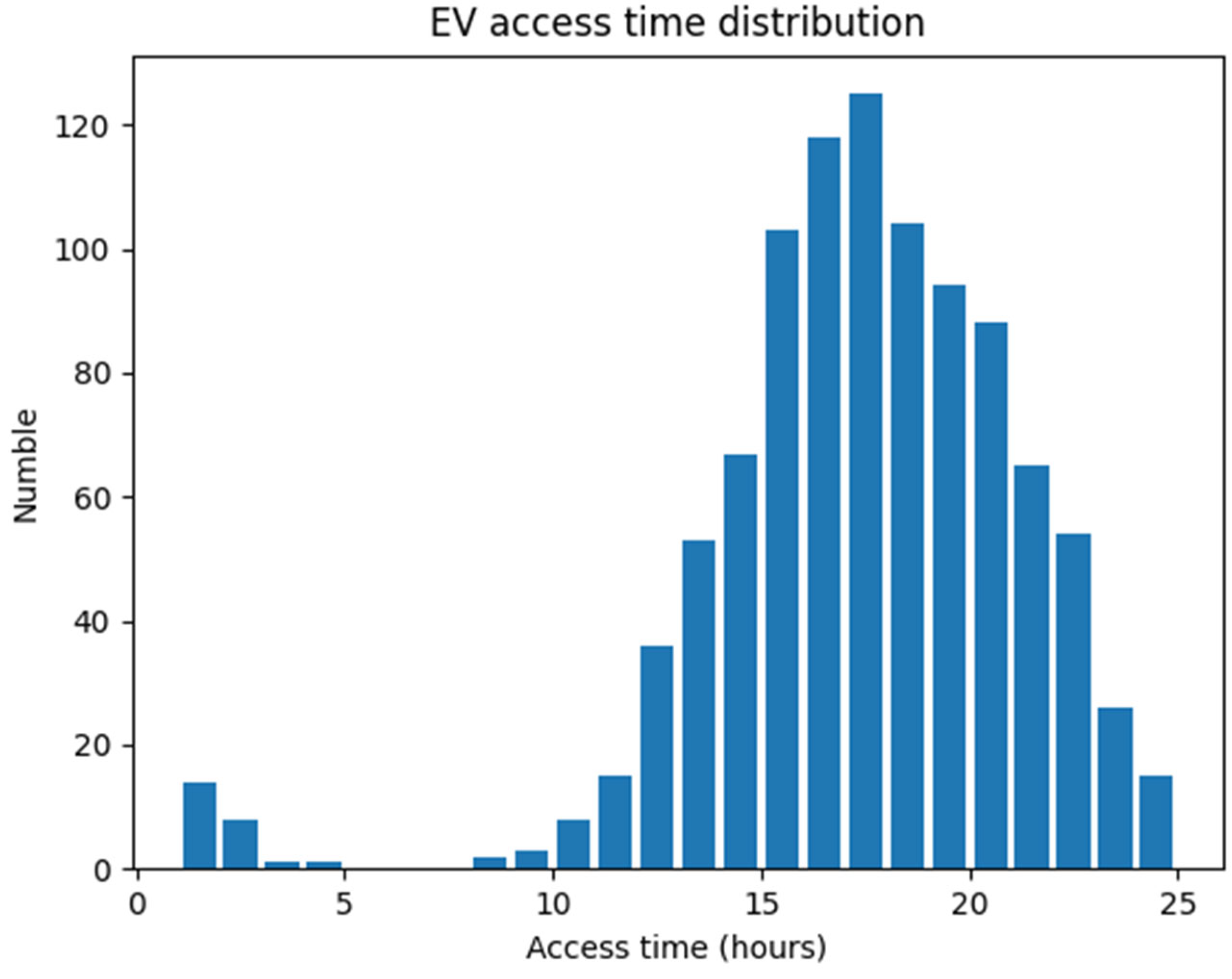
Table A3 presents the fuzzy affiliation function for estimating the number of EVs based on temperature, while Table A4 lists the parameters related to EVs as distributed spare capacity. The EV fleet is characterized by a weighted probability distribution across five battery capacities: 12 kWh (7.5%), 24 kWh (22%), 48 kWh (40.5%), 72 kWh (22.5%), and 96 kWh (7.5%). The contractual status between EVs and the grid is modelled using a weighted probability distribution: 20% drop out, 40% G2V, and 40% V2G. The contractually agreed energy capacity between EVs and the grid is set to 48 kWh. The grid connection time of each EV is determined using a customized cumulative distribution function, as illustrated in Figure A2.
Table A3. Membership function between temperature and number of electric vehicles.
Parameter NameDescription of ParameterParameter Range
Temp_centerCentral temperature of membership function[10, 20, 30] °C
Temp_stdStandard deviation of normal distribution in each temperature zone[3, 5, 3]
Temp_weightInfluence weight of each temperature zone on access intention[0.3, 1.0, 0.5]
NMaximum number of electric vehicles1000
TemperatureActual ambient temperatureObtained from NWP data
Table A4. Relevant parameters of electric vehicle simulation.
Parameter NameDescription of ParameterParameter Range
NMaximum number of electric vehicles1000
E max Battery capacityWeighted discrete distribution
S O C s t a r t Initial state of chargeU (0.2, 0.8)
t s t a r t Access time of electric vehicleCustom cumulative distribution function
P G , max Maximum discharge power3.3 kw
P L , max Maximum charging power3.3 kw
S O C exp Expected final SOC0.95
S O C m s Guaranteed SOC limit0.5
Figure A1 demonstrates battery energy constraints during charging and discharging of electric vehicles.
Figure A1. Constraint of charging and discharging process on electric power of electric vehicle.
Processes 13 03870 g0a1
Figure A2. Time distribution of electric vehicles connected to power grid.
Processes 13 03870 g0a2
Table A5 shows the parameters associated with the distributed energy storage with 10 units. The rest of the model parameters are shown in the table.
Table A5. Related parameters of distributed energy storage simulation.
Parameter NameDescription of ParameterParameter Range
NNumber of energy storage units10
S O C i n i t Rated capacity of energy storage unitU (500, 1400)
S O C m a x Maximum SOC0.95
S O C m i n Minimum SOC0.05
P ¯ c Maximum charging power200 kw
P ¯ d Maximum discharge power 200 kw
S O C i n i t Initial SOC of energy storageU (0.3, 0.7)
η c Energy storage charging efficiency0.95
η d Energy storage discharge efficiency0.95
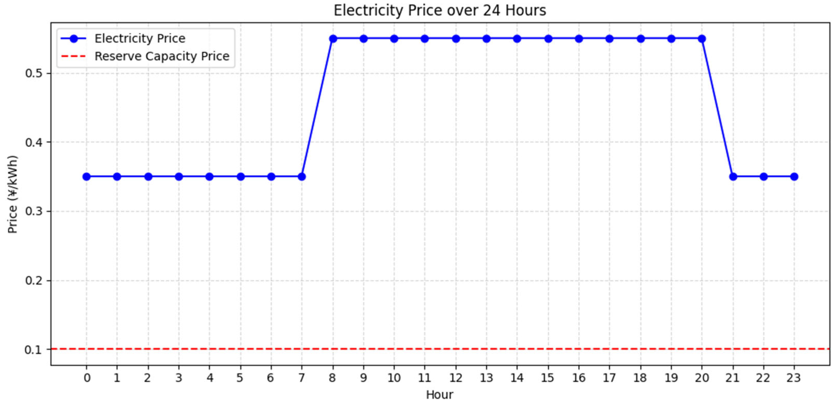
The reserve capacity of each type of distributed reserve resource is modelled by economic self-scheduling, and the specific power prices are shown in Figure A3. Both the upper and lower spare capacity prices are $0.1/kwh.
Figure A3. Reserve resource capacity price.
Processes 13 03870 g0a3
Figure A4. Prediction error of base learner based on Bayesian Optimization.
Processes 13 03870 g0a4
Figure A5. Hourly reserve capacity and meteorological features.
Processes 13 03870 g0a5

References

  1. Xu, C.X.; Chen, Z.X.; Zhu, W.J.; Zhi, J.Q.; Yu, Y.; Shi, C.F. Time-frequency spillover and early warning of climate risk in international energy markets and carbon markets: From the perspective of complex network and machine learning. Energy 2025, 318, 134857. [Google Scholar] [CrossRef]
  2. Cao, Y.; Yong, P.; Yu, J.; Yang, Z. Stacking algorithm based framework with strong generalization performance for ultra-short-term photovoltaic power forecasting. Energy 2025, 322, 135599. [Google Scholar] [CrossRef]
  3. Wang, Q.; Zhang, S.; Li, R. Artificial intelligence in the renewable energy transition: The critical role of financial development. Renew. Sustain. Energy Rev. 2026, 226, 116280. [Google Scholar] [CrossRef]
  4. Mohandes, B.; El Moursi, M.S.; Hatziargyriou, N.; El Khatib, S. A Review of Power System Flexibility with High Penetration of Renewables. IEEE Trans. Power Syst. 2019, 34, 3140–3155. [Google Scholar] [CrossRef]
  5. Sadeghi, H.; Shami, H.O.; Moazzami, M.; Ahmadi, G.; Toghraie, D.; Rezaei, M.; Dolatshahi, M.; Salahshour, S. Design an integrated strategic resource planning to analyze the development of renewable energy sources. Energy Strategy Rev. 2024, 53, 101427. [Google Scholar] [CrossRef]
  6. Kim, W.W.; Shin, J.S.; Kim, J.O. Operation Strategy of Multi-Energy Storage System for Ancillary Services. IEEE Trans. Power Syst. 2017, 32, 4409–4417. [Google Scholar] [CrossRef]
  7. Venkatesan, K.; Gouda, P.K.; Rath, B.B.; Krishnamoorthy, M. Optimal day-ahead scheduling of microgrid equipped with electric vehicle and distributed energy resources: SFO-CSGNN approach. J. Energy Storage 2024, 102, 113933. [Google Scholar] [CrossRef]
  8. Wang, Y.M.; Wang, Y.X.; Ni, J.N.; Zhang, H.D. Integration of smart buildings with high penetration of storage systems in isolated 100% renewable microgrids. J. Energy Storage 2025, 105, 114633. [Google Scholar] [CrossRef]
  9. Aliasghari, P.; Mohammadi-Ivatloo, B.; Alipour, M.; Abapour, M.; Zare, K. Optimal scheduling of plug-in electric vehicles and renewable micro-grid in energy and reserve markets considering demand response program. J. Clean. Prod. 2018, 186, 293–303. [Google Scholar] [CrossRef]
  10. Gopalan, S.A.; Sreeram, V.; Iu, H.H. A review of coordination strategies and protection schemes for microgrids. Renew. Sustain. Energy Rev. 2014, 32, 222–228. [Google Scholar] [CrossRef]
  11. Szostok, A.; Stanek, W. Thermo-ecological analysis of the power system based on renewable energy sources integrated with energy storage system. Renew. Energy 2023, 216, 119035. [Google Scholar] [CrossRef]
  12. Ghaemi, Z.; Tran, T.T.; Smith, A.D. Comparing classical and metaheuristic methods to optimize multi-objective operation planning of district energy systems considering uncertainties. Appl. Energy 2022, 321, 119400. [Google Scholar] [CrossRef]
  13. Pinto, E.S.; Serra, L.M.; Lázaro, A. Energy communities approach applied to optimize polygeneration systems in residential buildings: Case study in Zaragoza, Spain. Sustain. Cities Soc. 2022, 82, 103885. [Google Scholar] [CrossRef]
  14. Hong, J.T.; Hui, H.X.; Zhang, H.C.; Dai, N.Y.; Song, Y.H. Distributed Control of Large-Scale Inverter Air Conditioners for Providing Operating Reserve Based on Consensus with Nonlinear Protocol. IEEE Internet Things J. 2022, 9, 15847–15857. [Google Scholar] [CrossRef]
  15. Li, Y.; Yang, Z.; Li, G.Q.; Zhao, D.B.; Tian, W. Optimal Scheduling of an Isolated Microgrid with Battery Storage Considering Load and Renewable Generation Uncertainties. IEEE Trans. Ind. Electron. 2019, 66, 1565–1575. [Google Scholar] [CrossRef]
  16. Xiao, J.; Li, P.; Mao, Z.; Diao, H.; Li, J.; Tu, C. Multi-layer control strategy to enhance the economy and stability of battery energy storage system in wind farms. Int. J. Electr. Power Energy Syst. 2025, 169, 110776. [Google Scholar] [CrossRef]
  17. Dai, J.; Ding, C.; Yan, C.; Tang, Y.; Zhou, X.; Xue, F. Robust optimization method of power system multi resource reserve allocation considering wind power frequency regulation potential. Int. J. Electr. Power Energy Syst. 2024, 155, 109599. [Google Scholar] [CrossRef]
  18. Wang, Y.J.; Sun, Z.D.; Chen, Z.H. Development of energy management system based on a rule-based power distribution strategy for hybrid power sources. Energy 2019, 175, 1055–1066. [Google Scholar] [CrossRef]
  19. Wang, Y.; Gao, Q. Optimal Scheduling Considering Demand Response Based on Multi-Energy Complementary Distributed Integrated Energy Management System. In Proceedings of the 2024 3rd International Conference on Energy and Electrical Power Systems (ICEEPS), Guangzhou, China, 14–16 July 2024; pp. 248–252. [Google Scholar]
  20. Yu, G.; Cheng, B.; Xu, T.; Pan, J.; Chen, Y. Multi-level task network scheduling and electricity supply collaborative optimization under time-of-use electricity pricing. Comput. Ind. Eng. 2025, 203, 110952. [Google Scholar] [CrossRef]
  21. Hui, H.X.; Ding, Y.; Liu, W.D.; Lin, Y.; Song, Y.H. Operating reserve evaluation of aggregated air conditioners. Appl. Energy 2017, 196, 218–228. [Google Scholar] [CrossRef]
  22. Hong, J.T.; Hui, H.X.; Zhang, H.C.; Dai, N.Y.; Song, Y.H. Event-Triggered Consensus Control of Large-Scale Inverter Air Conditioners for Demand Response. IEEE Trans. Power Syst. 2022, 37, 4954–4957. [Google Scholar] [CrossRef]
  23. Pourmousavi, S.A.; Patrick, S.N.; Nehrir, M.H. Real-Time Demand Response Through Aggregate Electric Water Heaters for Load Shifting and Balancing Wind Generation. IEEE Trans. Smart Grid 2014, 5, 769–778. [Google Scholar] [CrossRef]
  24. Zhou, M.; Wang, M.; Li, J.F.; Li, G.Y. Multi-area Generation-reserve Joint Dispatch Approach Considering Wind Power Cross-regional Accommodation. CSEE J. Power Energy Syst. 2017, 3, 74–83. [Google Scholar] [CrossRef]
  25. Babahajiani, P.; Shafiee, Q.; Bevrani, H. Intelligent Demand Response Contribution in Frequency Control of Multi-Area Power Systems. IEEE Trans. Smart Grid 2018, 9, 1282–1291. [Google Scholar] [CrossRef]
  26. Qiu, H.F.; Gu, W.; You, F.Q. Bilayer Distributed Optimization for Robust Microgrid Dispatch with Coupled Individual-Collective Profits. IEEE Trans. Sustain. Energy 2021, 12, 1525–1538. [Google Scholar] [CrossRef]
  27. Habibi, M.; Vahidinasab, V.; Shafie-khah, M.; Catalao, J.P.S. Coordinated scheduling of energy storage systems as a fast reserve provider. Int. J. Electr. Power Energy Syst. 2021, 130, 106941. [Google Scholar] [CrossRef]
  28. Laslett, D.; Carter, C.; Creagh, C.; Jennings, P. A large-scale renewable electricity supply system by 2030: Solar, wind, energy efficiency, storage and inertia for the South West Interconnected System (SWIS) in Western Australia. Renew. Energy 2017, 113, 713–731. [Google Scholar] [CrossRef]
  29. Koltsaklis, N.E.; Knápek, J. Integrated market scheduling with flexibility options. Renew. Sustain. Energy Rev. 2025, 208, 115020. [Google Scholar] [CrossRef]
  30. Bluhm, H.; Gährs, S. Environmental assessment of prosumer digitalization: The case of virtual pooling of PV battery storage systems. J. Energy Storage 2023, 59, 106487. [Google Scholar] [CrossRef]
  31. Miyazaki, K.; Kobayashi, K.; Azuma, S.; Yamaguchi, N.; Yamashita, Y. Design and Value Evaluation of Demand Response Based on Model Predictive Control. IEEE Trans. Ind. Inform. 2019, 15, 4809–4818. [Google Scholar] [CrossRef]
  32. Li, Y.; Wang, R.N.; Yang, Z. Optimal Scheduling of Isolated Microgrids Using Automated Reinforcement Learning-Based Multi-Period Forecasting. IEEE Trans. Sustain. Energy 2022, 13, 159–169. [Google Scholar] [CrossRef]
  33. Ju, L.W.; Tan, Z.F.; Yuan, J.Y.; Tan, Q.K.; Li, H.H.; Dong, F.G. A bi-level stochastic scheduling optimization model for a virtual power plant connected to a wind-photovoltaic-energy storage system considering the uncertainty and demand response. Appl. Energy 2016, 171, 184–199. [Google Scholar] [CrossRef]
  34. Rezaei, N.; Pezhmani, Y.; Khazali, A. Economic-environmental risk-averse optimal heat and power energy management of a grid-connected multi microgrid system considering demand response and bidding strategy. Energy 2022, 240, 122844. [Google Scholar] [CrossRef]
  35. Ribó-Pérez, D.; Carrión, A.; García, J.R.; Bel, C.A. Ex-post evaluation of Interruptible Load programs with a system optimisation perspective. Appl. Energy 2021, 303, 117643. [Google Scholar] [CrossRef]
  36. Mousavi-Taghiabadi, S.M.; Sedighizadeh, M.; Zangiabadi, M.; Fini, A.S. Integration of wind generation uncertainties into frequency dynamic constrained unit commitment considering reserve and plug in electric vehicles. J. Clean. Prod. 2020, 276, 124272. [Google Scholar] [CrossRef]
  37. Zhao, C.Y.; Wang, J.H.; Watson, J.P.; Guan, Y.P. Multi-Stage Robust Unit Commitment Considering Wind and Demand Response Uncertainties. IEEE Trans. Power Syst. 2013, 28, 2708–2717. [Google Scholar] [CrossRef]
  38. Torkan, R.; Ilinca, A.; Ghorbanzadeh, M. A genetic algorithm optimization approach for smart energy management of microgrid. Renew. Energy 2022, 197, 852–863. [Google Scholar] [CrossRef]
  39. Mazidi, M.; Zakariazadeh, A.; Jadid, S.; Siano, P. Integrated scheduling of renewable generation and demand response programs in a microgrid. Energy Convers. Manag. 2014, 86, 1118–1127. [Google Scholar] [CrossRef]
  40. Jiang, B.Y.; Guo, C.X.; Chen, Z. Frequency Constrained Dispatch with Energy Reserve and Virtual Inertia from Wind Turbines. IEEE Trans. Sustain. Energy 2025, 16, 1340–1355. [Google Scholar] [CrossRef]
  41. Sadeghi, S.; Jahangir, H.; Vatandoust, B.; Golkar, M.A.; Ahmadian, A.; Elkamel, A. Optimal bidding strategy of a virtual power plant in day-ahead energy and frequency regulation markets: A deep learning-based approach. Int. J. Electr. Power Energy Syst. 2021, 127, 106646. [Google Scholar] [CrossRef]
  42. Gassar, A.A.A. Short-Term Energy Forecasting to Improve the Estimation of Demand Response Baselines in Residential Neighborhoods: Deep Learning vs. Machine Learning. Buildings 2024, 14, 2242. [Google Scholar] [CrossRef]
  43. Chen, R.H.; Yang, C.; Han, L.J.; Wang, W.D.; Ma, Y.; Xiang, C.L. Power reserve predictive control strategy for hybrid electric vehicle using recognition-based long short-term memory network. J. Power Sources 2022, 520, 230865. [Google Scholar] [CrossRef]
  44. Zheng, X.D.; Chen, H.B.; Jin, T. A new optimization approach considering demand response management and multistage energy storage: A novel perspective for Fujian Province. Renew. Energy 2024, 220, 119621. [Google Scholar] [CrossRef]
  45. Guo, Y.B.; Wang, J.Y.; Chen, H.X.; Li, G.N.; Liu, J.Y.; Xu, C.L.; Huang, R.G.; Huang, Y. Machine learning-based thermal response time ahead energy demand prediction for building heating systems. Appl. Energy 2018, 221, 16–27. [Google Scholar] [CrossRef]
  46. Li, J.B.; Chen, Z.Q.; Cheng, L.; Liu, X.F. Energy data generation with Wasserstein Deep Convolutional Generative Adversarial Networks. Energy 2022, 257, 124694. [Google Scholar] [CrossRef]
  47. Nyangon, J. Climate-Proofing Critical Energy Infrastructure: Smart Grids, Artificial Intelligence, and Machine Learning for Power System Resilience against Extreme Weather Events. J. Infrastruct. Syst. 2024, 30, 03124001. [Google Scholar] [CrossRef]
  48. Ji, Y.L.; Xu, Q.S.; Zhao, J.; Yang, Y.B.; Sun, L. Day-ahead and intra-day optimization for energy and reserve scheduling under wind uncertainty and generation outages. Electr. Power Syst. Res. 2021, 195, 107133. [Google Scholar] [CrossRef]
  49. Chen, X.P.; Lu, F.; Cheng, Y.P. Study on Reserve Capacity Optimization Model of Wind and Solar Power Generation System Based on Multi-Objective Optimization. In Proceedings of the 4th National Conference on Electrical, Electronics and Computer Engineering (NCEECE), Xi’an, China, 12–13 December 2016; pp. 71–79. [Google Scholar]
  50. Mueller, F.; Wörner, S.; Lygeros, J. Ramp-rate-constrained bidding of energy and frequency reserves in real market settings. arXiv 2018, arXiv:1804.03892. [Google Scholar]
  51. Xu, M.; Li, W.; Feng, Z.; Bai, W.; Jia, L.; Wei, Z. Economic Dispatch Model of High Proportional New Energy Grid-Connected Consumption Considering Source Load Uncertainty. Energies 2023, 16, 1696. [Google Scholar] [CrossRef]
  52. Li, Q.F.; Zhao, Y.H.; Yang, Y.W.; Zhang, L.T.; Ju, C. Demand-Response-Oriented Load Aggregation Scheduling Optimization Strategy for Inverter Air Conditioner. Energies 2023, 16, 337. [Google Scholar] [CrossRef]
  53. Bai, Z.Y.; Li, Z.W.; Zhang, Y.L.; Guo, Y.F.; Song, S. Model of Electric Water Heater and Influencing factors Analysis of Frequency Regulation Response Capability on Demand Side. In Proceedings of the 3rd IEEE International Electrical and Energy Conference (CIEEC), Beijing, China, 7–9 September 2019; pp. 827–833. [Google Scholar]
  54. Gabaldón, A.; García-Garre, A.; Ruiz-Abellón, M.C.; Guillamón, A. Modeling and Aggregation of Electric Water Heaters for the Development of Demand Response Using Grey Box Models. Appl. Sci. 2024, 14, 6258. [Google Scholar] [CrossRef]
  55. Cheng, J.; Wang, L.X.; Pan, T. Optimized Configuration of Distributed Power Generation Based on Multi-Stakeholder and Energy Storage Synergy. IEEE Access 2023, 11, 129773–129787. [Google Scholar] [CrossRef]
  56. Sonder, H.B.; Cipcigan, L.; Loo, C.U. Using Electric Vehicles and Demand Side Response to Unlock Distribution Network Flexibility. In Proceedings of the IEEE Milan PowerTech Conference, Milan, Italy, 23–27 June 2019. [Google Scholar]
  57. Zhou, C.; Qian, K.; Allan, M.; Zhou, W. Modeling of the Cost of EV Battery Wear Due to V2G Application in Power Systems. IEEE Trans. Energy Convers. 2011, 26, 1041–1050. [Google Scholar] [CrossRef]
  58. Mukhi, K.; Abate, A. An exact characterisation of flexibility in populations of electric vehicles. In Proceedings of the 2023 62nd IEEE Conference on Decision and Control (CDC), Singapore, 13–15 December 2023; pp. 6582–6587. [Google Scholar]
  59. Chen, Y.; Xu, J. Solar and wind power data from the Chinese State Grid Renewable Energy Generation Forecasting Competition. Sci. Data 2022, 9, 577. [Google Scholar] [CrossRef] [PubMed]
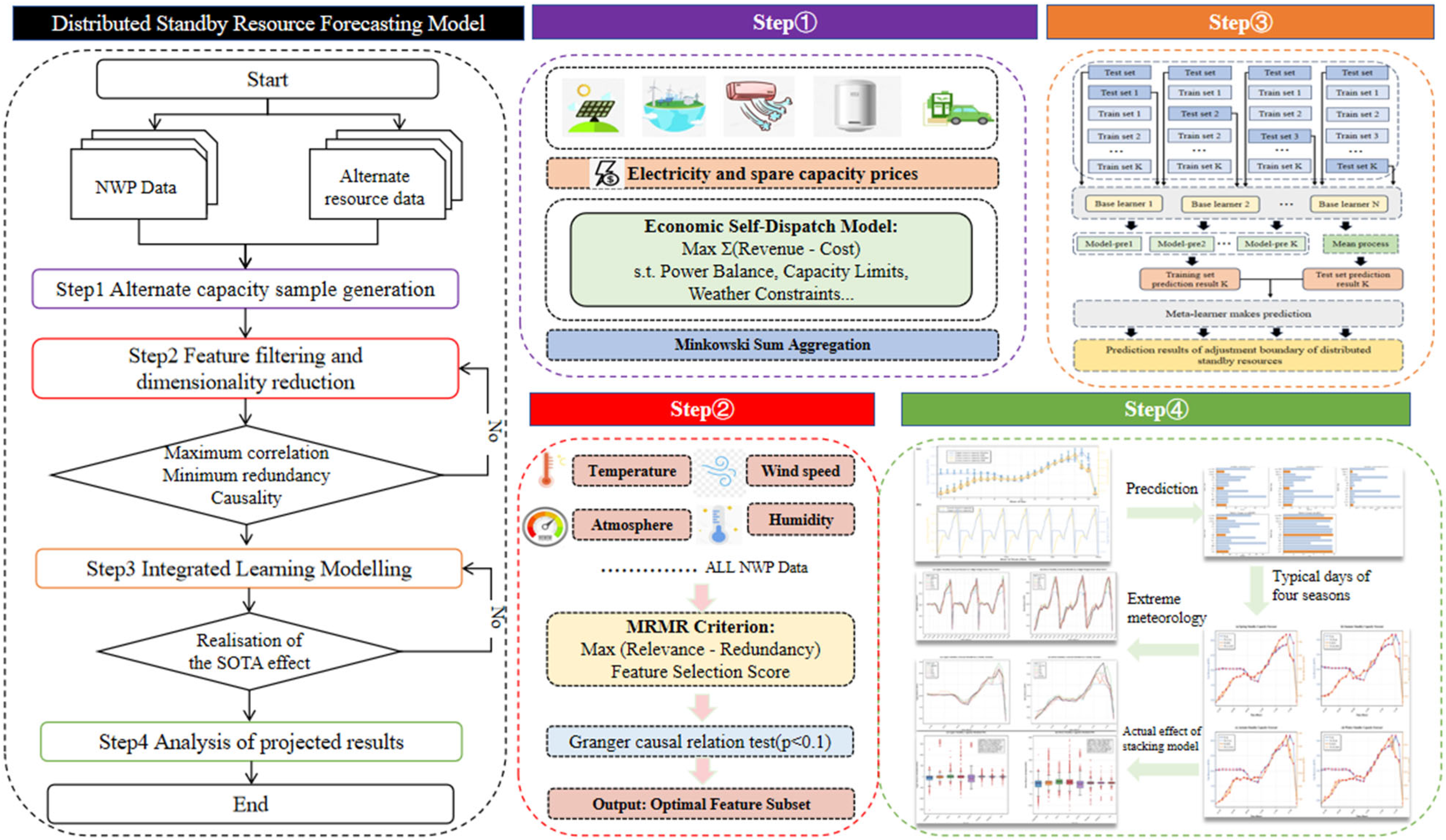
Figure 1. Research flow frame diagram.
Processes 13 03870 g001
Figure 2. Stacking integrated learning model structure diagram.
Processes 13 03870 g002
Figure 3. Statistical distribution and periodicity characteristics of distributed reserve resources. (a) indicates the intra-day distribution of distributed resources after reserve aggregation; (b) indicates the periodicity of reserve resources over the course of a week.
Processes 13 03870 g003
Figure 4. Prediction results for each candidate base learner.
Processes 13 03870 g004
Figure 5. Forecast results of upper reserve and lower reserve on typical days of four seasons. (ad) are spring, summer, autumn, and winter, respectively. The purple star markers represent the actual reserve values at each time point.
Processes 13 03870 g005
Figure 6. Comparison of the stacking model’s reserve resource prediction effects with other models under high temperature heatwave scenarios. (a) is the upper-reserve resource prediction effect; (b) is the lower-reserve resource prediction effect.
Processes 13 03870 g006
Figure 7. Comparison of the stacking model’s reserve resource prediction effect with other models in windy weather. (a) is the upper-reserve resource prediction effect; (b) is the lower-reserve resource prediction effect.
Processes 13 03870 g007
Figure 8. Comparison of the prediction errors of the models on the unknown dataset. (a) is the upper-reserve prediction error; (b) is the lower-reserve prediction error.
Processes 13 03870 g008
Table 1. Research gaps in existing studies.
MethodKey FocusLimitationsOur Improvement
MILP/Robust Optimization/Two-stage Stochastic Optimization
[22,23,24]
Physical modeling and coordinated schedulingHigh computational cost; difficult for large-scale systems; limited online adaptabilityCombines physical modelling with data-driven approach for scalable, flexible assessment
GRU/LSTM/RNN/RF/XGBoost/LightGBM
[27,28,29,30,31]
Data-driven prediction of reserve capacityHigh dependence on data quality; may lack interpretability and physical constraintsUses mRMR + Granger causality for feature selection; stacking ensemble improves accuracy and generalization
Existing meteorology-aware methods
[12,13,14,15,16,17,18,19]
Impact of weather on reserveOften single-resource focused; limited multi-source integrationProposes multi-source, meteorology-aware integrated framework for distributed resources
Stacking with mRMR and GrangerIntegrated prediction and evaluation under meteorological uncertainty/Provides planning and operational decision-support; handles multi-source, high-dimensional, nonlinear, weather-perturbed data; improves interpretability and generalization
Table 2. Feature selection results.
Feature
Name
Average Mutual
Information
Feature
Sorting
F Value
Up
p Value
Up
F Value Downp Value
Down
WindSpeed_wheel0.33570.0240.9983.6570.026 **
Wind_temperature0.101102.9910.018 **3.8160.010 ***
Wind_Atmosphere0.02537.3540.007 ***3.2490.011 **
Wind_humidity0.07152.2570.080 *1.9060.126
Direct irradiance0.26980.8340.3611.2100.298
Global irradiance0.26960.8330.3611.2130.297
Solar_temperature0.11525.2330.000 ***4.8480.028 **
Solar_Atmosphere0.01941.8310.1393.9400.020 **
WindPower0.33511.6370.1954.0440.018 **
Note: *** indicates significant at the 1% level. ** indicates significant at the 5% level. * indicates significant at the 10% level.
Table 3. Results of parameter settings for each candidate model.
ModelParameter SettingModelParameter Setting
LightGBMThe number of leaf nodes is 100; tree depth 5; the learning rate is 0.01; L1 regularization coefficient is 0.1; L2 regularization 0.95GBRThe number of trees is 100; Tree depth 5; The learning rate is 0.1; minimum sample 1 of leaf node; minimum sample of internal division node 2
XGBoostThe number of trees is 100; tree depth 5; L1 regularization coefficient is 0.1; L2 regularization 0.95; sample weight sum 2KNNNumber of neighbours 10; neighbour weight is uniform; calculate neighbour method auto
CatBoostThe number of trees is 100; the learning rate is 0.1; tree depth 5; L2 regularization coefficient 3; number of buckets 32MLPThe number of neurons in the first layer is 16, the number of neurons in the second layer is 16, the learning rate is 0.05, and the batch size is 64
SVRThe kernel function is Gaussian kernel; ε parameter 0.1; penalty parameter 1BayThe convergence threshold 1 × 10⁻⁶ and the prior parameters are 1 × 10⁻⁶
KANThe number of neurons is 32, the learning rate is 0.01 and the batch size is 64RNNThe number of neurons in the first layer is 64, the number of neurons in the second layer is 64, the learning rate is 0.01, and the batch size is 64
RFThe number of trees is 100; tree depth 5; minimum sample 1 of leaf node; minimum sample of internal division node 2LSTMThe number of neurons in the first layer is 64, the number of neurons in the second layer is 64, the learning rate is 0.01, and the batch size is 64
DTTree depth 5; minimum sample 1 of leaf node; minimum sample 2 of internal division nodes GRUThe number of neurons in the first layer is 64, the number of neurons in the second layer is 64, the learning rate is 0.01, and the batch size is 64
Table 4. Indicators of the outcome of the upper-reserve prediction for each type of integrated model.
Model NameMSERMSEMAEMAPER2Time(s)
CNN-BiLSTM700.33126.46416.8280.7490.997784.48
CNN-BiGRU710.78426.66116.0510.7710.997708.18
CNN-LSTM-Attention1223.48534.97824.7031.2470.995545.69
CNN-GRU-Attention891.42429.85717.8000.8570.997507.81
LSTM-KAN3313.50857.56330.1690.0090.98670.11
GRU-KAN2816.50253.07128.9570.0090.98869.41
Our966.76131.09319.3820.9190.996130.85
Table 5. Indicators of the outcome of the lower-reserve prediction for each type of integrated model.
Model NameMSERMSEMAEMAPER2Time(s)
CNN-BiLSTM3698.21260.81347.6861.0720.993758.97
CNN-BiGRU3975.01460.04850.2311.1260.992691.93
CNN-LSTM-Attention4246.42665.16547.7321.0520.991534.33
CNN-GRU-Attention4237.59965.09749.6141.1180.991497.55
LSTM-KAN15,052.415122.68871.4160.0120.96974.90
GRU-KAN16,897.812129.99276.5290.0130.96670.36
Our model4317.62565.70950.0571.1400.991133.71
Disclaimer/Publisher’s Note: The statements, opinions and data contained in all publications are solely those of the individual author(s) and contributor(s) and not of MDPI and/or the editor(s). MDPI and/or the editor(s) disclaim responsibility for any injury to people or property resulting from any ideas, methods, instructions or products referred to in the content.