Intelligent Frequency Control for Hybrid Multi-Source Power Systems: A Stepwise Expert-Teaching PPO Approach

Abstract

This paper proposes a stepwise expert-teaching reinforcement learning framework for intelligent frequency control in hydro–thermal–wind–solar–compressed air energy storage (CAES) integrated systems under high renewable energy penetration. The proposed method addresses the frequency stability challenge in low-inertia, high-volatility power systems, particularly in Southwest China, where large-scale renewable-energy-based energy bases are rapidly emerging. A load frequency control (LFC) model is constructed to serve as the training and validation environment, reflecting the dynamic characteristics of the hybrid system. The stepwise expert-teaching PPO (SETP) framework introduces a stepwise training mechanism in which expert knowledge is embedded to guide the policy learning process and training parameters are dynamically adjusted based on observed performance. Comparative simulations under multiple disturbance scenarios are conducted on benchmark systems. Results show that the proposed method outperforms standard proximal policy optimization (PPO) and traditional PI control in both transient response and coordination performance.

1. Introduction

To address global climate change, China aims to peak carbon emissions by 2030 and achieve carbon neutrality by 2060, with notable progress already made [1]. By the end of 2023, the Southwest region had built the country’s cleanest power grid, with hydro, wind, and solar capacity reaching 130 GW—nearly 80% of the total [2]. However, the large-scale integration of hydro–wind–solar–storage bases has reduced system inertia and increased frequency fluctuations [3]. This calls for coordinated frequency control strategies to fully tap the regulation potential of diverse resources within the base [4,5].

Frequency restoration in power systems primarily relies on automatic generation control (AGC), which generates the total regulation power through control loops and allocates it to individual regulating units based on predefined rules [6]. Although recent studies have introduced online parameter tuning and ultra-short-term optimization methods to enhance AGC’s control and dispatch performance, limitations remain in terms of adaptability and computational efficiency [7].

In recent years, reinforcement learning has been extensively studied in various areas of power systems, including system control [8], economic dispatch [9], microgrid energy management [10], and electricity market operations [11]. Owing to its “offline training–online deployment” paradigm, it has attracted significant attention in automatic generation control (AGC) applications, as this paradigm satisfies the 4–6 s dispatch cycle requirement and provides strong nonlinear approximation capability [12]. Study [13] has further deployed a DRL-based AGC strategy in a municipal distribution network through a virtual simulation system, preliminarily verifying the practical feasibility of this research direction.

Research on DRL for power allocation can be broadly categorized into two main directions:

• Enhancing conventional DRL algorithms to improve training efficiency and control performance in power dispatch tasks [14,15].
• Applying DRL techniques to achieve optimal power allocation for heterogeneous energy systems across various operating scenarios [16].

For the control layer, the literature primarily focuses on the following:

• Leveraging DRL to adaptively tune controller parameters, thereby improving the performance of AGC systems [17,18,19,20,21].
• Directly employing DRL agents as controllers to generate system-wide regulation commands [22,23,24,25,26].

Significant progress has been made in applying DRL to improve individual components; however, research on the holistic optimization of both control and allocation processes remains relatively limited [27]. Study [26] employs a heuristic algorithm to optimize the input weights of the state space in deep deterministic policy gradient (DDPG), thereby achieving improvements across both control and allocation. Nevertheless, this study is confined to power allocation between thermal power units and energy storage systems, which limits its applicability.

Among studies [14,15,16,17,18,19,20,21,22,23,24,25,26], most studies employ algorithms such as deep Q-Network (DQN) and DDPG, with only studies [16,25] adopting stochastic policy algorithms. Specifically, study [16] implements second-level power optimization and allocation of multiple types of energy storage resources in emergency ramping scenarios based on the PPO algorithm, which demonstrates stronger exploration capability and higher steady-state reward values compared with DDPG, twin delayed deep deterministic policy gradient (TD3), and other algorithms. Study [25] applies the SAC algorithm to realize distributed control of microgrids, and experimental results show that this method outperforms DDPG in key performance metrics such as settling time, frequency deviation, and robustness. Study [28], using a classical reinforcement learning environment, systematically analyzes and compares algorithms, revealing that PPO achieves higher sample efficiency, greater stability, and easier implementation. These studies indicate that stochastic policy algorithms hold substantial application potential; however, their applicability and performance in LFC tasks have yet to be thoroughly investigated and validated [29].

Despite the strong self-learning and decision-making capabilities demonstrated by DRL algorithms such as DDPG, SAC, and PPO, their applications in power systems remain limited due to poor training stability, high sensitivity to hyperparameters, insufficient algorithmic robustness, and low training efficiency [30,31,32]. In load frequency control (LFC) tasks, the rationality and safety of training scenarios must also be carefully considered. On the one hand, if the training environment is overly idealized or the disturbance design is inappropriate, the agent’s generalization ability and training stability under complex operating conditions will deteriorate significantly [33]; on the other hand, reinforcement learning relies on trial-and-error exploration, and during the early stages of training, the agent is prone to entering unsafe regions, generating a large number of ineffective samples and resulting in slow policy convergence [34].

To address the above issues, researchers have proposed several improvements to standard reinforcement learning algorithms. Study [30] introduces a delayed update mechanism to mitigate training instability; study [31] enhances sample efficiency by optimizing the experience replay mechanism; study [24] employs demonstrators in the early stage of training to provide expert samples, thereby improving the agent’s guidance and robustness; and study [35] proposes a multi-stage training strategy based on task complexity, offering new insights into the application of DRL in LFC tasks.

Building upon the aforementioned research progress, this study investigates an energy base located in Southwest China and proposes an intelligent frequency control strategy based on the SETP framework. First, a load frequency control model incorporating hydropower, thermal power, wind power, photovoltaic generation, and compressed air energy storage is developed according to the base’s generation mix. Then, building upon the PPO algorithm, the SETP framework is constructed with adjustable disturbance scenarios, a staged training mechanism, a safe action mapping mechanism, and an expert-guided mechanism. These features ensure the rational design of training environments, enhance training stability, reduce ineffective samples, and guarantee the effective implementation of the learned policy. Finally, comparative experiments are conducted under both weak and strong disturbance scenarios to evaluate the control performance of PPO, SETP, and conventional PI control. In addition, the regulation mileage of each strategy is analyzed, thereby verifying the control effort of the proposed method.

2. LFC Model of Hydro–Thermal–Wind–Solar–CAES System

2.1. Generator–Load Model

Given the small-signal disturbance scenario in this study, the generator and load dynamics in the s-domain are represented as follows:

$$\Delta f^{\ast }={\displaystyle \frac{1}{2H_{\mathrm{eq}}s+D}}\Delta P_{\mathrm{u}}^{\ast }$$

(1)

where $\Delta f^{\ast }$ denotes the per-unit frequency deviation; $H_{\mathrm{eq}}$ denotes the equivalent inertia time; D denotes the load damping constant; and $\Delta P_{\mathrm{u}}^{\ast }$ denotes the per-unit power imbalance.

A single-area LFC model is established as the simulation environment, where thermal power units, hydro power units, and a CAES provide inertial support to the system. The constant is calculated using Equation (2), following the formulation in [36].

$$H_{\mathrm{eq}}={\displaystyle \frac{{\displaystyle \sum _{i=1}^n}(H_i·S_{\mathrm{b},i})}{{\displaystyle \sum _{i=1}^n}{S}_{\mathrm{b},i}}}$$

(2)

where $H_i$ denotes the inertia constant of unit i; $S_{\mathrm{b},i}$ denotes the rated capacity of unit i; and $H_{\mathrm{eq}}$ denotes the equivalent inertia constant of the system. And the subscript $i=1–6$ corresponds to the thermal unit, CAES, hydro unit, wind farm, PV station, and battery energy storage system (BESS).

2.2. Primary Frequency Control

2.2.1. Governor with Speed Droop Characteristic

Since the simulation environment consists of multiple power sources, droop governors are employed. Taking a thermal power unit as an example, its s-domain model is given as follows:

$$\Delta P_{\mathrm{v},\mathrm{thermal}}^{\ast }=-{\displaystyle \frac{1}{R_{\mathrm{thermal}}}}·{\displaystyle \frac{1}{1+s{T}_{\mathrm{g}}}}\Delta f^{\ast }$$

(3)

where $R_{\mathrm{thermal}}$ denotes the droop rate; $T_{\mathrm{g}}$ denotes the governor time constant; and $\Delta P_{\mathrm{v},\mathrm{thermal}}$ denotes the valve position.

2.2.2. Hydro Turbine Governor

Considering the water hammer effect, the hydro turbine governor incorporates a transient droop compensation component, and its s-domain model is given by

$$\Delta P_{\mathrm{v},\mathrm{hydro}}^{\ast }=-{\displaystyle \frac{1}{R_{\mathrm{hydro}}}}·{\displaystyle \frac{1}{1+s{T}_{\mathrm{g}}}}·{\displaystyle \frac{1+s{T}_{\mathrm{R}}}{1+s(R_{\mathrm{T}}/R_{\mathrm{H}})T_{\mathrm{R}}}}\Delta f^{\ast }$$

(4)

where $T_{\mathrm{R}}$ denotes the dashpot time constant; $R_{\mathrm{T}}$ denotes the temporary droop coefficient; $R_{\mathrm{H}}$ denotes the permanent droop coefficient; and $R_{\mathrm{hydro}}$ denotes the hydro power unit.

2.2.3. Synthetic Inertia Control Strategy

The wind and solar resources involved in this paper are all equipped with energy storage systems, connected to the grid through converters, and decoupled from the grid side and thus unable to actively provide inertia support to the grid. This paper considers that their primary frequency regulation process adopts a synthetic inertia control strategy combining droop control and virtual inertia control:

$$\Delta P_{\mathrm{PF}}^{\mathrm{ref}}=K_{\mathrm{df}}{\displaystyle \frac{\mathrm{d}\Delta f^{\ast }}{\mathrm{d}t}}+K_{\mathrm{pf}}\Delta f^{\ast }$$

(5)

where $\Delta P_{\mathrm{PF}}^{\mathrm{ref}}$ denotes the primary frequency regulation reference; $K_{\mathrm{df}}$ and $K_{\mathrm{pf}}$ denote the virtual inertia control coefficient and droop control coefficient, respectively.

2.3. Conventional Power Sources

2.3.1. Hydro Turbine

The s-domain model of the hydro turbine is given by

$$\Delta P_{\mathrm{m},\mathrm{hydro}}^{\ast }={\displaystyle \frac{1-s{T}_{\mathrm{W}}}{1+0.5s{T}_{\mathrm{W}}}}\Delta P_{\mathrm{v},\mathrm{hydro}}^{\ast }$$

(6)

where $T_{\mathrm{W}}$ denotes the water starting time constant and $\Delta P_{\mathrm{m},\mathrm{hydro}}^{\ast }$ denotes per-unit mechanical power deviation of the hydro unit.

2.3.2. Steam Turbine

The reheat steam turbine is modeled in the s-domain as follows:

$$\Delta P_{\mathrm{m},\mathrm{thermal}}^{\ast }={\displaystyle \frac{1+s{F}_{\mathrm{HP}}{T}_{\mathrm{RH}}}{1+s{T}_{\mathrm{RH}}}}·{\displaystyle \frac{1}{1+s{T}_{\mathrm{CH}}}}\Delta P_{\mathrm{v},\mathrm{thermal}}^{\ast }$$

(7)

where $F_{\mathrm{HP}}$ denotes the high-pressure turbine power fraction; $T_{\mathrm{RH}}$ denotes the reheater time constant; $T_{\mathrm{CH}}$ denotes the crossover time constant; and $\Delta P_{\mathrm{m},\mathrm{thermal}}^{\ast }$ denotes per-unit mechanical power deviation of the thermal unit.

2.4. Renewable Energy Sources

Photovoltaic Power Stations and Wind Farms

The converter response speed of photovoltaic power stations and wind farms is relatively fast. This paper considers their power response characteristics as first-order inertial components:

$$\left\{\begin{array}{c}{P}_{\mathrm{wt}}={\displaystyle \frac{1}{1+s{T}_{\mathrm{c}}}}{P}_{\mathrm{wt}}^{\mathrm{ref}}\hfill \\ P_{\mathrm{pv}}={\displaystyle \frac{1}{1+s{T}_{\mathrm{c}}}}{P}_{\mathrm{pv}}^{\mathrm{ref}}\hfill \end{array}\right.$$

(8)

where $P_{\mathrm{wt}}$ and $P_{\mathrm{pv}}$ denote the actual output power of the wind farm and photovoltaic power station, respectively; $P_{\mathrm{wt}}^{\mathrm{ref}}$ and $P_{\mathrm{pv}}^{\mathrm{ref}}$ denote the power references for the wind farm and the photovoltaic power station, respectively; and $T_{\mathrm{c}}$ denotes the converter control time constant.

2.5. Energy Storage Systems

2.5.1. CAES

In this study, CAES participates in system frequency regulation through expansion power generation. Since the day-ahead and intra-day dispatch processes ensure a 5–10% operating margin for the CAES reservoir pressure and thermal storage temperature, and their variations remain within 5% during the training horizon considered in this study, the changes in reservoir pressure and thermal storage temperature are neglected. Therefore, the influences of the thermal storage devices, heat exchange systems, and air storage reservoirs are not taken into account. Following the formulation in [37], the output power and outlet temperature of the i-th expander are expressed as

$$\left\{\begin{array}{c}{T}_{\mathrm{tx},i}=T_{\mathrm{td},i}\left[1-\left(1-{\pi }_{\mathrm{t},i}^{{\displaystyle \frac{1-k}{k}}}\right){\eta }_{\mathrm{ti}}\right]\hfill \\ P_{\mathrm{tm},i}=c_p{\dot{m}}_t\left(T_{\mathrm{td},i}-T_{\mathrm{tx},i}\right)\hfill \end{array}\right.$$

(9)

where $T_{\mathrm{tx},i}$ denotes the outlet gas temperature of the i-th expander; $T_{\mathrm{td},i}$ denotes the inlet gas temperature of the i-th expander; ${\pi }_{\mathrm{t},i}$ denotes the expansion ratio of the i-th expander; $k=c_p/c_v$ denotes the specific heat ratio, also known as the adiabatic index, where $c_p$ and $c_v$ are the constant-pressure and constant-volume specific heats of air, respectively; ${\dot{m}}_t$ is the air mass flow rate of the expander; $P_{\mathrm{tm},i}$ is the shaft power of the i-th expander; and ${\eta }_{\mathrm{ti}}$ is the isentropic efficiency.

CAES regulates the expander power by controlling ${\dot{m}}_t$ to respond to the power reference. The s-domain model of its air flow control system is

$$\left\{\begin{array}{c}{P}_{\mathrm{tm}}={\displaystyle \sum _i}{P}_{\mathrm{tm},i}\hfill \\ {\dot{m}}_t=\left(P_{\mathrm{CAES}}^{\mathrm{ref}}-P_{\mathrm{tm}}\right)\left(K_{\mathrm{tp}}+{\displaystyle \frac{K_{\mathrm{ti}}}{s}}\right){\displaystyle \frac{1}{1+s{T}_{\mathrm{TD}}}}{\displaystyle \frac{1}{1+s{T}_{\mathrm{AV}}}}\hfill \end{array}\right.$$

(10)

where $T_{\mathrm{TD}}$ and $T_{\mathrm{AV}}$ are the turbine gas discharge time delays and $P_{\mathrm{CAES}}^{\mathrm{ref}}$ is the power reference for the CAES. The control block diagram is shown in Figure 1.

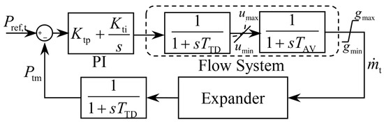
Figure 1. CAES control system block diagram.

2.5.2. BESS

The converter model of the electrochemical energy storage station is similar to Equation (8); its state of charge (SOC) is calculated by the following equation and must satisfy the constraints shown below to avoid overcharging and over-discharging:

$$\left\{\begin{array}{cc}{\displaystyle x_{\mathrm{soc}}=x_{{\mathrm{soc}}_0}-{\int }_{t_0}^t{\displaystyle \frac{P_{\mathrm{bess}}}{\eta }}\mathrm{d}\tau ,}\hfill & P_{\mathrm{bess}}>0\hfill \\ {\displaystyle x_{\mathrm{soc}}=x_{{\mathrm{soc}}_0}-{\int }_{t_0}^t\eta P_{\mathrm{bess}}\mathrm{d}\tau ,}\hfill & P_{\mathrm{bess}}\le 0\hfill \end{array}\right.$$

(11)

$$P_{\mathrm{bess}}=\left\{\begin{array}{cc}min(P_{\mathrm{bess}}^{\mathrm{ref}},0)\hfill & x_{\mathrm{soc}}\ge x_{\mathrm{soc}}^{\max }\hfill \\ P_{\mathrm{bess}}^{\mathrm{ref}}\hfill & x_{\mathrm{soc}}^{\min }<x_{\mathrm{soc}}<x_{\mathrm{soc}}^{\max }\hfill \\ max(P_{\mathrm{bess}}^{\mathrm{ref}},0)\hfill & x_{\mathrm{soc}}\le x_{\mathrm{soc}}^{\min }\hfill \end{array}\right.$$

(12)

where $x_{\mathrm{soc}}$, $x_{{\mathrm{soc}}_0}$, $x_{\mathrm{soc}}^{\min }$, and $x_{\mathrm{soc}}^{\max }$ denote the current, initial, minimum, and maximum SOC; $P_{\mathrm{bess}}$ and $P_{\mathrm{bess}}^{\mathrm{ref}}$ denote the actual and reference power; and $\eta$ is the charging/discharging efficiency.

2.6. Conventional AGC Control Strategy Based on PI Control

AGC employs PI control to obtain the total regulation power, with the input of PI control being the area control error; subsequently, rules such as “proportional to adjustable capacity” are used to allocate power to each unit.

2.6.1. Area Control Error (ACE)

Since the simulation environment in this paper is a single area, the AGC control mode adopts constant frequency control, and the calculation formula for the area control error is [38]:

$$x_{\mathrm{ACE}}=-B(f-f_0)$$

(13)

where $x_{\mathrm{ACE}}$ denotes the area control error, where $x_{\mathrm{ACE}}>0$ indicates excessive generation in this area; B denotes the bias factor of the control area; f is the current system frequency; and $f_0$ is the system reference frequency. The value of B is selected according to the composite frequency response characteristic, as detailed in Appendix A.1.

2.6.2. Power Dispatch Strategy

The control power is dispatched proportionally according to the available regulation capacity of each unit as follows:

$${\alpha }_i=\left\{\begin{array}{cc}{\displaystyle \frac{P_i^{\mathrm{avail},\mathrm{up}}}{{\displaystyle \sum _{i=1}^n}{P}_i^{\mathrm{avail},\mathrm{up}}}}\hfill & x_{\mathrm{ACE}}<0\hfill \\ {\displaystyle \frac{P_i^{\mathrm{avail},\mathrm{down}}}{{\displaystyle \sum _{i=1}^n}{P}_i^{\mathrm{avail},\mathrm{down}}}}\hfill & x_{\mathrm{ACE}}\ge 0\hfill \end{array}\right.$$

(14)

where $P_i^{\mathrm{avail},\mathrm{up}}$ and $P_i^{\mathrm{avail},\mathrm{down}}$ represent the upward and downward regulation capacities of unit i, respectively.

2.7. AGC Control Strategy Based on DRL

The DRL-based AGC strategy adopts an offline training and online deployment paradigm, where neural networks parameterize the control policy to enhance adaptability and generalization in frequency regulation. In this paradigm, the agent replaces conventional AGC control and allocation, interacting with the environment to collect experience for offline learning and policy evaluation. A training framework based on PPO, enhanced with expert knowledge integration and a staged training mechanism, is developed to improve convergence efficiency and policy performance, with implementation details provided in Section 3.

The LFC model constructed based on Section 2.1, Section 2.2, Section 2.3, Section 2.4, Section 2.5, Section 2.6 and Section 2.7 is illustrated in Figure 2; the corresponding parameters are listed in Table A1.

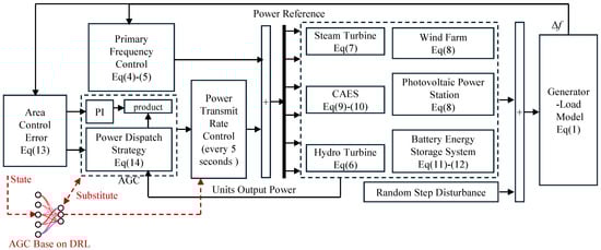
Figure 2. LFC for hydro–wind–solar–CAES integrated energy base.

3. Stepwise Expert-Teaching PPO Framework for LFC

3.1. PPO Training Procedure

PPO is an on-policy reinforcement learning algorithm that enhances training stability by restricting the magnitude of policy updates. Its application in load frequency control follows four key steps:

1. Interaction with Environment. The PPO agent interacts with the LFC environment under the current policy ${\pi }_{\theta }$ to collect trajectory data. The number of time steps per collection round is defined as the experience horizon, which determines the batch size used in policy updates.

2. Advantage Estimation. To assess the quality of actions within the collected trajectories, the Generalized Advantage Estimation (GAE) method is applied:

$${\widehat{A}}_t={\delta }_t+\left(\gamma \lambda \right){\delta }_{t+1}+\cdots +{\left(\gamma \lambda \right)}^{T-t+1}{\delta }_{T-1}$$

(15)

where ${\delta }_t=r_t+\gamma V\left(s_{t+1}\right)-V\left(s_t\right)$ denotes the temporal difference (TD) error; $\gamma$ denotes the discount factor; and $\lambda$ denotes the GAE smoothing factor.

3. Network Updates. The collected trajectories are split into mini-batches and used to update the actor and critic networks over multiple epochs using the Adam optimizer. The actor network is updated using the clipped surrogate loss:

$$L^{\mathrm{CLIP}}\left(\theta \right)={\mathbb{E}}_t\left[min\left(r_t\left(\theta \right){\widehat{A}}_t,\mathrm{clip}(r_t\left(\theta \right),1-ϵ,1+ϵ){\widehat{A}}_t\right)+\beta \mathcal{H}\left[{\pi }_{\theta }\left(s_t\right)\right]\right]$$

(16)

where $r_t\left(\theta \right)$ denotes the importance sampling ratio; $ϵ$ denotes the clipping factor; and $\beta$ denotes the entropy coefficient. The critic is trained by minimizing the value function loss:

$$L^{\mathrm{VF}}\left(\varphi \right)={\mathbb{E}}_t\left[{\left(V_{\varphi }\left(s_t\right)-{\widehat{V}}_t\right)}^2\right]$$

(17)

where ${\widehat{V}}_t={\widehat{A}}_t+V_{{\varphi }_{\mathrm{old}}}\left(s_t\right)$ denotes the estimated return, decoupled from current updates to enhance stability.

4. Policy Iteration. Steps 1 to 3 are repeated iteratively until the policy converges or a maximum number of training episodes is reached.

3.2. Reinforcement Learning Environment Design

3.2.1. State and Action Spaces

At each time step t, the agent receives an observation vector ${\mathbf{s}}_t$ composed of power deviations, power references, and the ACE:

$${\mathbf{s}}_t={\left[\Delta {\mathbf{P}}_t,{\mathbf{P}}_t^{\mathrm{ref}},x_{\mathrm{ACE},t}\right]}^{\top }$$

(18)

where $\Delta {\mathbf{P}}_t\in {\mathbb{R}}^6$ and ${\mathbf{P}}_t^{\mathrm{ref}}\in {\mathbb{R}}^6$ denote the power deviations and reference values of six energy sources and $x_{\mathrm{ACE},t}$ represents the area control error at time step t. The action vector is defined as follows:

$${\mathbf{a}}_t={\left[u_t^{\mathrm{thermal}},u_t^{\mathrm{CAES}},u_t^{\mathrm{hydro}},u_t^{\mathrm{WT}},u_t^{\mathrm{PV}},u_t^{\mathrm{BESS}}\right]}^{\top }$$

(19)

where each $u_t^i$ denotes the secondary frequency regulation command for the i-th energy resource at time t.

3.2.2. Reward Function

The reward function consists of three components: $r_1$ penalizing frequency deviations; $r_2$ suppressing oscillations in the agent’s output; and $r_3$ reflecting the cost of frequency regulation.

$$\begin{array}{cc}\hfill r_t& =r_1+r_2+r_3\hfill \\ \hfill r_1& =-{\lambda }_{\mathrm{ACE}}·\left|x_{\mathrm{ACE},t}\right|\hfill \\ \hfill r_2& =-{\lambda }_{\mathrm{act}}·\left|a_t-a_{t-1}\right|\hfill \\ \hfill r_3& =-{\lambda }_{\mathrm{eff}}·{\displaystyle \sum _{i=1}^n}{d}_i\left(t\right)\hfill \end{array}$$

(20)

where $x_{\mathrm{ACE},t}$ denotes the real-time ACE at time step t; $a_t$ and $a_{t-1}$ denote the agent’s control outputs at time steps t and $t-1$, respectively; $d_i\left(t\right)$ denotes the regulation mileage of unit i at time step t, and its calculation formula is provided in Appendix A.3; and ${\lambda }_{\mathrm{ACE}}$, ${\lambda }_{\mathrm{act}}$, and ${\lambda }_{\mathrm{eff}}$ denote the corresponding weighting factors.

3.2.3. Actor and Critic Network Architecture

The critic network is first constructed to estimate the state-value function $V\left(s\right)$, as shown in Figure 3.

Figure 3. Critic network architecture.

The actor network, shown in Figure 4, adopts a shared-body and dual-branch architecture. The shared body extracts state features via two fully connected layers with ReLU activations. The mean branch applies a tanh activation to normalize the output actions, while the standard deviation branch uses a softplus activation followed by a clipping layer to ensure numerical stability.

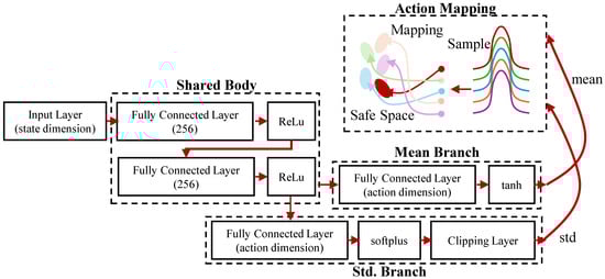
Figure 4. Actor network architecture.

The final action is sampled from a Gaussian distribution and mapped to the safe action domain through a linear transformation, defined as follows:

$${\mathbf{a}}_{\mathrm{safe}}={\displaystyle \frac{{\mathbf{a}}_{\mathrm{raw}}+\mathbf{1}}{2}}\left({\mathbf{a}}_{max}-{\mathbf{a}}_{min}\right)+{\mathbf{a}}_{min}$$

(21)

where ${\mathbf{a}}_{\mathrm{raw}}$ denotes the normalized action vector sampled from the Gaussian policy and ${\mathbf{a}}_{min},{\mathbf{a}}_{max}$ represent the element-wise lower and upper bounds of the action domain, respectively; the corresponding parameters are listed in Table A2.

As implemented, PPO is updated using Equation (22) and SETP employs Equations (22) and (23).

$$\begin{array}{cc}\hfill \theta & \leftarrow \theta -{\alpha }_{\theta }{\nabla }_{\theta }{L}^{\mathrm{CLIP}}\left(\theta \right)\hfill \\ \hfill \varphi & \leftarrow \varphi -{\alpha }_{\varphi }{\nabla }_{\varphi }{L}^{\mathrm{VF}}\left(\varphi \right)\hfill \end{array}$$

(22)

$$\theta \leftarrow \theta -{\alpha }_{\theta }^{\mathrm{expert}}{\nabla }_{\theta }{L}^{\mathrm{expert}}\left(\theta \right)$$

(23)

where $\theta$ and $\varphi$ denote the parameters of the actor and critic networks, respectively; ${\alpha }_{\theta }$, ${\alpha }_{\varphi }$, and ${\alpha }_{\theta }^{\mathrm{expert}}$ are the learning rates of the actor, critic, and expert-guided actor updates; $L^{\mathrm{CLIP}}\left(\theta \right)$ is the PPO surrogate loss; $L^{\mathrm{VF}}\left(\varphi \right)$ is the critic value function loss; and $L^{\mathrm{expert}}\left(\theta \right)$ is the expert loss.

3.2.4. Disturbance Scenario Generation

To generate disturbance scenarios that are both stochastic and physically feasible, we adopt a truncated Gaussian sampling strategy with stepwise and cumulative constraints. Let the cumulative disturbance up to step $i-1$ be defined as follows:

$$S_{i-1}={\displaystyle \sum _{k=1}^{i-1}}{ϵ}_k$$

Then, the disturbance at step i is sampled according to the following rules:

$$\left\{\begin{array}{c}{ϵ}_i\sim \mathcal{N}(\mu ,{\sigma }^2)\hfill \\ {ϵ}_{min}\le {ϵ}_i\le {ϵ}_{max}\hfill \\ S_{min}\le S_{i-1}+{ϵ}_i\le S_{max}\hfill \end{array}\right.$$

(24)

where $\mu$ and $\sigma$ denote the mean and standard deviation of the Gaussian distribution, $[{ϵ}_{min},{ϵ}_{max}]$ defines the allowable range for each step, and $[S_{min},S_{max}]$ specifies the bounds for the cumulative disturbance; the corresponding parameters are listed in Table A3. The rationale and sensitivity analysis of these parameters are presented in Appendix A.7.

3.3. High-Quality Operational Data Generation

To generate high-quality expert control data for guiding and behavior cloning, this paper employs a multi-swarm particle swarm optimization (MPSO) algorithm to tune the PI controller parameters $K_{\mathrm{p}}$ and $K_{\mathrm{i}}$ across a wide range of disturbance scenarios. By introducing multiple interacting sub-swarms, MPSO enhances population diversity and global search capability.

To balance frequency regulation accuracy and control smoothness, the fitness function is defined as follows:

$$J={\int }_0^T\left({\lambda }_1|\Delta f\left(t\right)|+{\lambda }_2\left|u\left(t\right)\right|\right)dt$$

(25)

where $\Delta f\left(t\right)$ denotes the system frequency deviation, $u\left(t\right)$ is the controller output, and ${\lambda }_1$ and ${\lambda }_2$ are weighting coefficients that trade off precision and stability, set to $0.7$ and $0.3$, respectively.

3.4. Expert-Guided and Stepwise Mechanism

In the stepwise training mechanism, the entire training process is divided into multiple phases. In each phase, experts dynamically adjust the training parameters, agent parameters, disturbance parameters, and reward parameters based on evaluations such as the reward curve. When the training process encounters convergence difficulties, a behavioral cloning mechanism can be triggered to assist policy convergence and enhance training stability.

Once triggered, mini-batches are randomly sampled from the expert dataset to perform supervised updates. The loss function is defined as follows:

$$L_{\mathrm{expert}}\left(\theta \right)={\displaystyle \frac{1}{N}}{\displaystyle \sum _{i=1}^N}{∥{\pi }_{\theta }\left(s_i\right)-a_i^{\mathrm{expert}}∥}^2+{\beta }_{\mathrm{expert}}{\parallel \theta \parallel }^2$$

(26)

where ${\pi }_{\theta }\left(s_i\right)$ is the action predicted by the current policy network, $a_i^{\mathrm{expert}}$ is the expert action, N is the batch size, and ${\beta }_{\mathrm{expert}}$ is the L2 regularization coefficient.

The overall architecture of the expert-guided PPO training framework, including disturbance generation, expert data construction, and integrated training with supervision, is illustrated in Figure 5, and the related training hyperparameters are provided in Table A4. The rationale and sensitivity analysis of these parameters are presented in Appendix A.7.

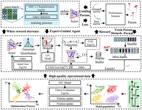
Figure 5. Expert-guided PPO framework.

4. Results and Discussion

To highlight the advantages of the SETP, this study conducts comparative experiments under both small- and large-disturbance scenarios using the established LFC model. The control behavior and performance of SETP, standard PPO, and traditional PI control are thoroughly evaluated. Furthermore, the trade-offs between control performance and control effort are analyzed for SETP and PPO.

4.1. Comparative Analysis of Training Processes for SETP and PPO

PPO is trained separately under weak and strong disturbance scenarios, with the corresponding learning curves shown in Figure 6, where Figure 6a corresponds to the weak disturbance case and Figure 6b to the strong disturbance case. In each figure, episode reward represents the total reward obtained in each episode, and average reward is its moving average, reflecting the steady improvement in overall performance; Episode Q0 depicts the action-value estimation, and the close overlap of the two curves in the later stage indicates that the policy training has essentially converged. In both scenarios, the reward function, as defined in (20), incorporates $r_1$ and $r_2$, while $r_3$ is omitted to avoid further increasing the training difficulty given the limited frequency regulation performance. During training, $r_2$ helps suppress frequent action oscillations in the early stage, but in the later stage, it inhibits the improvement in $r_1$.

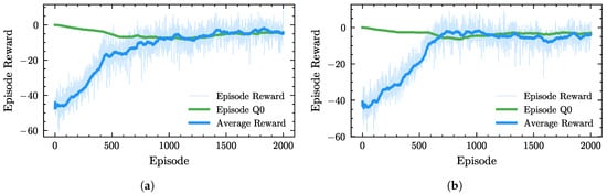
Figure 6. PPO training processes under weak and strong disturbances. (a) PPO training process under weak disturbances. (b) PPO training process under strong disturbances.

In contrast, the proposed SETP adopts a stepwise training strategy. The disturbance standard deviation gradually transitions from weak to strong disturbances, enabling a single training process to cover a broader range of disturbance conditions. The reward function coefficients are dynamically adjusted across stages, and after jointly considering $r_1$, $r_2$, and $r_3$, the coefficient of $r_2$ is reduced to zero once training converges, as shown in Figure 7.

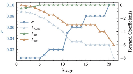
Figure 7. Variation in $\sigma$ and reward coefficients in stepwise training.

The effectiveness of this strategy is reflected in the training curves: as shown in Figure 8a, the expert-guidance loss decreases steadily throughout training, and although the reward curve changes little in the later stage, the policy remains stable despite continuous changes in environment difficulty and reward coefficients, demonstrating strong adaptability. Figure 8b further shows that the IAE decreases consistently over the entire training process, indicating a gradual reduction in frequency deviation, while the regulation mileage increases with improving regulation performance and is further optimized after performance stabilizes.

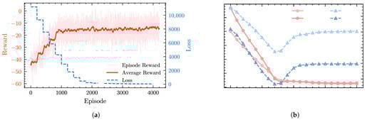
Figure 8. Training performance of SETP. (a) Reward and loss curves during SETP training. (b) Evolution of IAE and regulation mileage during SETP training.

4.2. Adaptability of Control Strategies Under Weak and Strong Disturbances

This study analyzes the control performance of SETP, fixed PI, and PPO under weak and strong disturbance scenarios. The outputs and commands of each unit are provided in Figure A1. As shown in the figures, SETP and fixed PI exhibit similar trends, whereas PPO presents a noticeably stronger overshoot.

In the following, we further compare the three strategies from the perspective of system frequency. In the weak disturbance scenario, the applied disturbance is illustrated in Figure 9. As shown in Figure 10, the proposed SETP exhibits a rapid frequency recovery after each disturbance, with smooth transients and a small overshoot, entering and stably maintaining within the $\pm 0.05$ Hz range in a short period of time. This demonstrates superior dynamic response capability and steady-state performance. In contrast, although the original PPO converged during training, its post-disturbance recovery is slower and accompanied by pronounced overshoot and undershoot, indicating insufficient stability in its dynamic regulation process. The conventional fixed PI shows larger steady-state deviations and sustained oscillations, with overall regulation performance significantly inferior to that of SETP.

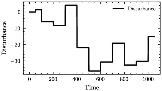
Figure 9. Disturbance profiles under weak disturbance conditions.

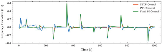
Figure 10. Frequency deviation profile under weak disturbance conditions.

Table 1 further confirms the advantages of SETP in dynamic regulation accuracy and steady-state stability, as observed in the frequency deviation profiles of Figure 10, with the calculation formulas of these metrics provided in Appendix A.6. Specifically, SETP achieves the lowest IAE and ITAE, indicating the smallest cumulative frequency deviation both over the entire process and within the weighted disturbance windows; the lowest RMS deviation, reflecting the smallest overall fluctuation amplitude; the shortest mean settling time, indicating the fastest frequency recovery; and the lowest steady-state standard deviation, demonstrating stable steady-state performance.

Table 1. Key performance metrics in the weak disturbance scenario. Lower is better for all entries.

Strategy	IAE	ITAE	RMS	Settle Time	Steady Std
SETP	238.067 *	1255.642 *	0.069 *	60.280 *	0.053 *
PPO	383.772	1919.096	0.075	65.590	0.056
Fixed PI	306.048	1661.821	0.073	62.830	0.059

* Best (lowest) value in the column.

Figure 11a shows the radar chart derived from Table 1 after min–max normalization. The contour of SETP encloses those of PPO and fixed PI in most metrics, indicating a clear comparative advantage.

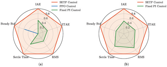
Figure 11. Performance metrics (IAE, ITAE, RMS, Settle Time, and Steady Std) under weak and strong disturbances. (a) Weak disturbances. (b) Strong disturbances.

In the strong disturbance scenario, the disturbance amplitude is larger ($\sigma =0.1$), as illustrated in Figure A2. In the weak disturbance scenario, the applied disturbance is illustrated in Figure 9. As shown in Figure 10, the proposed SETP achieves rapid frequency recovery after each disturbance, with smooth transients and minimal overshoot, entering and stably maintaining within the $\pm 0.05$ Hz range in a short time. This reflects both superior dynamic response capability and steady-state performance. In contrast, although the original PPO converges during training, its post-disturbance recovery is slower and exhibits pronounced overshoot and undershoot, indicating limited stability in dynamic regulation. The conventional fixed PI suffers from larger steady-state deviations and sustained oscillations, with overall regulation performance significantly inferior to that of SETP.

Quantitative results in Table 1 further confirm SETP’s advantages in both dynamic regulation accuracy and steady-state stability, consistent with the frequency deviation profiles. Specifically, SETP achieves the lowest IAE and ITAE, indicating the smallest cumulative frequency deviation over the entire process and within the weighted disturbance windows; the lowest RMS deviation, reflecting the smallest fluctuation amplitude; the shortest mean settling time, indicating the fastest recovery; and the lowest steady-state standard deviation, demonstrating stable steady-state performance. The radar chart in Figure 11a visually reinforces this advantage, with the contour of SETP enclosing those of PPO and fixed PI in most metrics.

In the strong disturbance scenario ($\sigma =0.1$), as illustrated in Figure A2, SETP maintains these advantages, continuing to outperform PPO and fixed PI with faster recovery, smoother transients, and smaller steady-state deviations, as shown in the frequency deviation profiles of Figure A3, the performance metrics in Table 2, and the radar chart in Figure 11b, demonstrating robustness under more severe operating conditions.

Table 2. Key performance metrics in the strong disturbance scenario. Lower is better for all entries.

Strategy	IAE	ITAE	RMS	Settle Time	Steady Std
SETP	324.655 *	1733.886 *	0.090 *	61.690 *	0.077 *
PPO	519.486	2810.826	0.110	70.220	0.087
Fixed PI	420.935	2302.876	0.096	64.910	0.084

* Best (lowest) value in the column.

Overall, across both weak and strong disturbance conditions, SETP consistently delivers faster frequency recovery, reduced oscillations, and improved steady-state stability, confirming its adaptability and effectiveness under varying operating conditions.

4.3. Analysis of Control Effort in SETP Control

As shown in Figure 12a,b, the cumulative regulation mileage of SETP is consistently and significantly lower than that of the fixed PI control in both weak and strong disturbance scenarios. Under weak disturbances, the regulation mileage of SETP is reduced by approximately 22% compared to the fixed PI control, with the entire curve remaining at a lower level, indicating that SETP achieves rapid frequency recovery and steady-state maintenance while effectively reducing the frequency and magnitude of control actions. Under strong disturbances, even with a notably higher overall regulation demand, SETP still achieves an approximately 22% reduction in regulation mileage, demonstrating a clear reduction in control effort under harsher operating conditions. Overall, SETP not only surpasses conventional strategies in dynamic and steady-state performance but also effectively reduces unnecessary control actions, thereby significantly lowering the overall control effort in long-term operation.

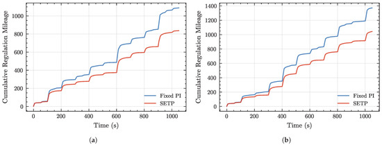
Figure 12. Regulation mileage comparison under weak and strong disturbances. (a) Regulation mileage under weak disturbances. (b) Regulation mileage under strong disturbances.

5. Conclusions

This study focuses on the frequency control requirements of a hydropower–wind–solar–compressed air clean energy base and proposes SETP, which integrates PPO with a stepwise training strategy and expert guidance mechanism. The framework is evaluated in both weak and strong disturbance scenarios, analyzing control performance and regulation mileage economic efficiency, leading to the following conclusions:

• Compared with the PPO algorithm, SETP adopts a stepwise training strategy that progresses from easier to more difficult scenarios, allowing a single training process to cover multiple operating conditions. By incorporating expert guidance, it further addresses diverse control requirements and significantly enhances training stability.
• In terms of control performance, SETP consistently demonstrates faster frequency recovery, smaller overshoot, and superior steady-state characteristics under various disturbance conditions. Compared with fixed PI control, SETP reduces the IAE by approximately 22% in the weak disturbance scenario and 23% in the strong disturbance scenario, while also achieving significantly improved average frequency recovery time and RMS deviation in both cases.
• In terms of regulation mileage, SETP achieves a reduction of approximately 22% compared to conventional PI control in both weak and strong disturbance scenarios, indicating lower control effort and smoother actuator responses.

The proposed SETP framework establishes a general paradigm for DRL-based frequency control in clean energy systems. By integrating PPO, safe action mapping, and expert guidance, it achieves strong adaptability and practicality. Future work will extend the framework to larger multi-energy systems to further validate its scalability and real-world applicability.

Appendix A.1

The frequency bias factor B is obtained by aggregating the frequency response characteristics of all participating resources on the system base. The equivalent droop coefficient $R_{\mathrm{eq}}$ is defined as

$${\displaystyle \frac{1}{R_{\mathrm{eq}}}}=\sum _i{\displaystyle \frac{S_{b,i}}{S_B}}{G}_i,$$

(A1)

where $S_{b,i}$ is the rated capacity of the i-th unit, $S_B$ is the system base capacity, and $G_i$ denotes the steady-state frequency–power conversion gain, with $G_i=1/R_i$ for synchronous units and $G_i=K_{\mathrm{pf},i}$ for inverter-based resources such as wind, PV, and BESSs. The bias factor is then given by

$$B={\displaystyle \frac{1}{R_{\mathrm{eq}}}}+D,$$

(A2)

where D is the load damping constant.

In this study, the rated capacities of thermal, CAES, hydro, wind, PV, and BESS units are $\{100,100,400,400,200,100\}$ MW, respectively, with a total system capacity of $S_B=1300$ MW. The droop coefficients are set as $R_{\mathrm{thermal}}=0.2$, $R_{\mathrm{CAES}}=0.2$, and $R_{\mathrm{hydro}}=0.5$. The proportional coefficients of the synthetic inertia control strategy are set as $K_{\mathrm{pf},\mathrm{wind}}=K_{\mathrm{pf},\mathrm{PV}}=K_{\mathrm{pf},\mathrm{BESS}}=2$. Substituting these values into the above equation yields

$${\displaystyle \frac{1}{R_{\mathrm{eq}}}}=2.4615,B=2.4615+0.5=2.9615\left(\mathrm{pu}/\mathrm{pu}\right).$$

(A3)

Appendix A.2

Table A1. Parameters of the LFC model.

Symbol	Value	Symbol	Value
$H_{\mathrm{eq}}\left[\mathrm{s}\right]$	1.42	$D\left[\mathrm{pu}\right]$	0.5
$S_{\mathrm{b},i}\left[\mathrm{MW}\right]$	100, 100, 400, 400, 200, 100	$H_i\left[\mathrm{s}\right]$	1.5, 0.5, 4.1, 0, 0, 0
$R_{\mathrm{thermal}}$	0.2	$T_{\mathrm{g}}\left[\mathrm{s}\right]$	0.05
$R_{\mathrm{hydro}}$	0.5	$T_{\mathrm{R}}\left[\mathrm{s}\right]$	5
$R_{\mathrm{T}}$	0.38	$R_{\mathrm{H}}$	0.05
$K_{\mathrm{df}}$	1	$K_{\mathrm{pf}}$	2
$T_{\mathrm{W}}\left[\mathrm{s}\right]$	1	$F_{\mathrm{HP}},T_{\mathrm{RH}},T_{\mathrm{CH}}$	0.3, 7, 0.3
$T_{\mathrm{c}}\left[\mathrm{s}\right]$	0.2	$T_{\mathrm{td},1}{[}^{\circ }\mathrm{C}],T_{\mathrm{tx},1}{[}^{\circ }\mathrm{C}],{\pi }_{\mathrm{t},1}$	193, 38, 4.6
$T_{\mathrm{td},2}{[}^{\circ }\mathrm{C}],T_{\mathrm{tx},2}{[}^{\circ }\mathrm{C}],{\pi }_{\mathrm{t},2}$	193, 43, 5.0	$T_{\mathrm{td},3}{[}^{\circ }\mathrm{C}],T_{\mathrm{tx},3}{[}^{\circ }\mathrm{C}],{\pi }_{\mathrm{t},3}$	193, 41, 4.7
${\eta }_{\mathrm{t}1},{\eta }_{\mathrm{t}2},{\eta }_{\mathrm{t}3}$	0.90, 0.92, 0.92	$K_{\mathrm{tp}}$	0.00058
$K_{\mathrm{ti}}$	0.000318	$T_{\mathrm{TD}}\left[\mathrm{s}\right]$	0.3
$T_{\mathrm{AV}}\left[\mathrm{s}\right]$	0.1	$R_{\mathrm{CAES}}$	0.2
$x_{\mathrm{soc}}0$	0.5	$x_{\mathrm{soc}}^{\min },x_{\mathrm{soc}}^{\max }$	0.2, 0.8
$\eta$	0.95	$B[\mathrm{pu}/\mathrm{pu}]$	2.9615
$P_i^{\mathrm{avail},\mathrm{up}}\left[\mathrm{MW}\right]$	50, 50, 120, 40, 20, 100	$P_i^{\mathrm{avail},\mathrm{down}}\left[\mathrm{MW}\right]$	−10, −30, −120, −40, −20, −100
${\lambda }_{\mathrm{mile}}$	1	$S_i^{\mathrm{perf}}$	0.34, 0.45, 0.55, 0.7, 0.7, 0.7

Table A1. Parameters of the LFC model.

Symbol	Value	Symbol	Value
$H_{\mathrm{eq}}\left[\mathrm{s}\right]$	1.42	$D\left[\mathrm{pu}\right]$	0.5
$S_{\mathrm{b},i}\left[\mathrm{MW}\right]$	100, 100, 400, 400, 200, 100	$H_i\left[\mathrm{s}\right]$	1.5, 0.5, 4.1, 0, 0, 0
$R_{\mathrm{thermal}}$	0.2	$T_{\mathrm{g}}\left[\mathrm{s}\right]$	0.05
$R_{\mathrm{hydro}}$	0.5	$T_{\mathrm{R}}\left[\mathrm{s}\right]$	5
$R_{\mathrm{T}}$	0.38	$R_{\mathrm{H}}$	0.05
$K_{\mathrm{df}}$	1	$K_{\mathrm{pf}}$	2
$T_{\mathrm{W}}\left[\mathrm{s}\right]$	1	$F_{\mathrm{HP}},T_{\mathrm{RH}},T_{\mathrm{CH}}$	0.3, 7, 0.3
$T_{\mathrm{c}}\left[\mathrm{s}\right]$	0.2	$T_{\mathrm{td},1}{[}^{\circ }\mathrm{C}],T_{\mathrm{tx},1}{[}^{\circ }\mathrm{C}],{\pi }_{\mathrm{t},1}$	193, 38, 4.6
$T_{\mathrm{td},2}{[}^{\circ }\mathrm{C}],T_{\mathrm{tx},2}{[}^{\circ }\mathrm{C}],{\pi }_{\mathrm{t},2}$	193, 43, 5.0	$T_{\mathrm{td},3}{[}^{\circ }\mathrm{C}],T_{\mathrm{tx},3}{[}^{\circ }\mathrm{C}],{\pi }_{\mathrm{t},3}$	193, 41, 4.7
${\eta }_{\mathrm{t}1},{\eta }_{\mathrm{t}2},{\eta }_{\mathrm{t}3}$	0.90, 0.92, 0.92	$K_{\mathrm{tp}}$	0.00058
$K_{\mathrm{ti}}$	0.000318	$T_{\mathrm{TD}}\left[\mathrm{s}\right]$	0.3
$T_{\mathrm{AV}}\left[\mathrm{s}\right]$	0.1	$R_{\mathrm{CAES}}$	0.2
$x_{\mathrm{soc}}0$	0.5	$x_{\mathrm{soc}}^{\min },x_{\mathrm{soc}}^{\max }$	0.2, 0.8
$\eta$	0.95	$B[\mathrm{pu}/\mathrm{pu}]$	2.9615
$P_i^{\mathrm{avail},\mathrm{up}}\left[\mathrm{MW}\right]$	50, 50, 120, 40, 20, 100	$P_i^{\mathrm{avail},\mathrm{down}}\left[\mathrm{MW}\right]$	−10, −30, −120, −40, −20, −100
${\lambda }_{\mathrm{mile}}$	1	$S_i^{\mathrm{perf}}$	0.34, 0.45, 0.55, 0.7, 0.7, 0.7

Table A2. Safe layer parameters.

Parameter	Symbol	Value
Action domain lower bound	${\mathbf{a}}_{min}$	$[-10,-30,-120,-40,-20,-100]$
Action domain upper bound	${\mathbf{a}}_{max}$	$[50,50,120,40,20,100]$

Table A2. Safe layer parameters.

Parameter	Symbol	Value
Action domain lower bound	${\mathbf{a}}_{min}$	$[-10,-30,-120,-40,-20,-100]$
Action domain upper bound	${\mathbf{a}}_{max}$	$[50,50,120,40,20,100]$

Table A3. Key parameters for disturbance scenario generation.

Parameter Name	Symbol	Value
Mean of Gaussian distribution	$\mu$	0
Standard deviation of Gaussian distribution	$\sigma$	[0.005, 0.1]
Minimum disturbance increment	${ϵ}_{min}$	−0.021
Maximum disturbance increment	${ϵ}_{max}$	0.021
Minimum cumulative disturbance	$S_{min}$	−0.24
Maximum cumulative disturbance	$S_{max}$	0.29

Table A3. Key parameters for disturbance scenario generation.

Parameter Name	Symbol	Value
Mean of Gaussian distribution	$\mu$	0
Standard deviation of Gaussian distribution	$\sigma$	[0.005, 0.1]
Minimum disturbance increment	${ϵ}_{min}$	−0.021
Maximum disturbance increment	${ϵ}_{max}$	0.021
Minimum cumulative disturbance	$S_{min}$	−0.24
Maximum cumulative disturbance	$S_{max}$	0.29

Table A4. Hyperparameters for PPO and SETP algorithms.

Algorithm	Symbol	Value
PPO	${\alpha }_{\theta },{\alpha }_{\varphi }$	$2\times {10}^{-5},1\times {10}^{-5}$
	Experience horizon	1500
	$ϵ$	0.4
	$\beta$	0.01
	$\gamma$	0.92
	$\lambda$	0.92
	${\lambda }_{\mathrm{ACE}},{\lambda }_{\mathrm{act}}$	$-2,-0.6$
SETP	${\beta }_{\mathrm{expert}}$	$1\times {10}^{-5}$
	${\lambda }_{\mathrm{ACE}},{\lambda }_{\mathrm{act}},{\lambda }_{\mathrm{eff}}$	not fixed values
	${\alpha }_{\mathrm{expert}}$	$1\times {10}^{-6}$
	${\alpha }_{\theta },{\alpha }_{\varphi }$	$1\times {10}^{-6},5\times {10}^{-5}$
	Experience horizon	1500
	$ϵ$	0.3
	$\beta$	0.01
	$\gamma$	0.98
	$\lambda$	0.98

Table A4. Hyperparameters for PPO and SETP algorithms.

Algorithm	Symbol	Value
PPO	${\alpha }_{\theta },{\alpha }_{\varphi }$	$2\times {10}^{-5},1\times {10}^{-5}$
	Experience horizon	1500
	$ϵ$	0.4
	$\beta$	0.01
	$\gamma$	0.92
	$\lambda$	0.92
	${\lambda }_{\mathrm{ACE}},{\lambda }_{\mathrm{act}}$	$-2,-0.6$
SETP	${\beta }_{\mathrm{expert}}$	$1\times {10}^{-5}$
	${\lambda }_{\mathrm{ACE}},{\lambda }_{\mathrm{act}},{\lambda }_{\mathrm{eff}}$	not fixed values
	${\alpha }_{\mathrm{expert}}$	$1\times {10}^{-6}$
	${\alpha }_{\theta },{\alpha }_{\varphi }$	$1\times {10}^{-6},5\times {10}^{-5}$
	Experience horizon	1500
	$ϵ$	0.3
	$\beta$	0.01
	$\gamma$	0.98
	$\lambda$	0.98

Appendix A.3

$$d_i\left(t\right)=S_i^{\mathrm{perf}}·{\lambda }_{\mathrm{mile}}·\left|P_i^{\mathrm{out}}\left(t\right)-P_i^{\mathrm{out}}(t-1)\right|$$

(A4)

where $P_i^{\mathrm{out}}\left(t\right)$ denotes the actual output power of unit i at time t and ${\lambda }_{\mathrm{mile}}$ denotes the regulation mileage price.

Appendix A.4

Figure A1. Power responses and commands of three control strategies under weak and strong disturbances. (a) SETP control, weak disturbances. (b) PPO control, weak disturbances. (c) Fixed PI control, weak disturbances. (d) SETP control, strong disturbances. (e) PPO control, strong disturbances. (f) Fixed PI control, strong disturbances.

Appendix A.5

Figure A2. Disturbance profiles under strong disturbance conditions.

Figure A3. Frequency deviation profile under strong disturbance conditions.

Appendix A.6

$$\left\{\begin{array}{c}\mathrm{IAE}={\displaystyle \frac{1}{N}}{\sum }_{n=1}^N\left|\Delta f\left(n\right)\right|,\hfill \\ \mathrm{ITAE}={\displaystyle {\sum }_{i=1}^M}\left[\sum _{t\in {\mathcal{W}}_i}t·\left|\Delta f\left(t\right)\right|·\Delta t\right],\hfill \\ \mathrm{RMS}=\sqrt{{\displaystyle \frac{1}{N}}{\sum }_{n=1}^N{\left(\Delta f\left(n\right)\right)}^2},\hfill \\ \mathrm{Settle}\mathrm{Time}={\displaystyle \frac{1}{M}}{\displaystyle {\sum }_{i=1}^M}{\tau }_i,{\tau }_i=min\left\{t\in {\mathcal{W}}_i|\left|\Delta f\left(t^{\prime }\right)\right|<\epsilon ,\forall t^{\prime }\ge t\right\},\hfill \\ \mathrm{Steady}\mathrm{Std}=\sqrt{{\displaystyle \frac{1}{N_s}}{\sum }_{n=N-N_s+1}^N{\left(\Delta f\left(n\right)-{\overline{\Delta f}}_{\mathrm{steady}}\right)}^2},\hfill \end{array}\right.$$

(A5)

where $\Delta f\left(t\right)=f\left(t\right)-f_0$ denotes the frequency deviation from the nominal frequency $f_0$; N is the total number of samples with a sampling interval of $\Delta t$; M is the number of disturbance events, and ${\mathcal{W}}_i$ represents the time window corresponding to the i-th disturbance; $\epsilon$ is the settling band threshold (e.g., 0.05 Hz); $N_s$ is the number of samples in the steady-state period, and ${\overline{\Delta f}}_{\mathrm{steady}}$ is the corresponding mean frequency deviation.

Appendix A.7. Rationality and Sensitivity Analysis of Parameter Selection

The parameters listed in Table A4 can be categorized into three groups:

(1)

PPO algorithm parameters, including the actor network learning rate ${\alpha }_{\theta }$, experience horizon, clipping factor $ϵ$, entropy coefficient, discount factor, and trade-off coefficient;

(2)

SETP algorithm parameters, which include all PPO parameters as well as the expert learning rate;

(3)

Coefficients in the reward function, namely ${\lambda }_{\mathrm{ACE}}$, ${\lambda }_{\mathrm{act}}$, and ${\lambda }_{\mathrm{eff}}$.

PPO algorithm parameters

For the parameter configuration of the PPO algorithm, this study conducts systematic training and comparative analysis of several key hyperparameters to evaluate their impacts on the reward function and determine the optimal parameter combination listed in Table A4.

Figure A4a presents the smoothed reward curves of the PPO agent. It can be observed that a smaller learning rate (e.g., $\alpha =1\times {10}^{-6}$) leads to slower learning and a lower final average reward, while an excessively large learning rate (e.g., $\alpha =1\times {10}^{-4}$) causes excessive policy update amplitudes and results in policy collapse. A moderate learning rate ($\alpha =5\times {10}^{-6}$–$6\times {10}^{-5}$) enables faster convergence to a better policy within fewer iterations. Figure A4b also shows that the PPO agent achieves the smallest fluctuation in episode reward when $\alpha =2\times {10}^{-5}$.

Figure A4c illustrates the effect of different experience horizon (EH) settings on the PPO training process. The results indicate that a large EH causes significant oscillations and keeps the episode reward at a relatively low level, while a small EH also leads to high fluctuations.

Figure A4d demonstrates the influence of different clipping factors on the PPO agent. The results show that an overly small clipping factor may restrict the policy optimization capability of the PPO algorithm, whereas a larger clipping factor performs better in the long run.

Figure A4e presents the effects of different entropy coefficients on PPO training. The results show that smaller entropy coefficients (0.005 and 0.01) achieve higher rewards, while larger entropy coefficients cause the agent to over-explore, resulting in a lower final reward.

Figure A4f shows the effect of $\gamma$ and $\lambda$ on the PPO agent. The results indicate that a smaller $\gamma$ focuses more on short-term rewards, enabling faster convergence but potentially limiting policy performance, while a larger $\gamma$ emphasizes long-term rewards, leading to slower convergence and a lower final reward.

SETP algorithm parameters

The SETP algorithm introduces an expert learning mechanism within the PPO framework, where the expert learning process also updates the parameters of the action network. Since the expert dataset contains approximately 64,800 samples, while the reinforcement learning process generates about 360,000 samples, and the quality of reinforcement learning data is relatively low in the early training stage, the network is updated five times during reinforcement learning but only once during expert learning, which is dominated by high-quality expert data. Therefore, in the expert learning stage, a higher learning rate is adopted for the actor network, while a lower learning rate is used in the reinforcement learning stage to balance the influence of the two types of data on network updates and maintain overall training stability.

Figure A4. Comparison of average episode rewards of the PPO agent under different parameter settings. (a) Average episode reward under different learning rates. (b) Reward under different learning rates. (c) Average episode reward of the PPO agent under different experience horizons. (d) Average episode reward of the PPO agent under different clipping factors. (e) Average episode reward of the PPO agent under different entropy coefficients. (f) Average episode reward of the PPO agent under different discount factors and trade-off coefficients.

Coefficients in the reward function

In the design of the reward function, the parameters ${\lambda }_{\mathrm{ACE}}$, ${\lambda }_{\mathrm{act}}$, and ${\lambda }_{\mathrm{eff}}$ are used to adjust the penalty weights associated with frequency deviation, differences between consecutive actions, and regulation mileage, respectively. In the PPO algorithm, these three parameters are set as fixed values. As shown in the experimental results, when only ${\lambda }_{\mathrm{ACE}}$ is applied, the agent’s output actions tend to exhibit high-frequency oscillations. Introducing ${\lambda }_{\mathrm{act}}$ effectively suppresses these oscillations but makes the agent’s policy more conservative, reducing its responsiveness to frequency disturbances and thus affecting control performance. To balance control performance and output smoothness, a smaller coefficient for ${\lambda }_{\mathrm{act}}$ is selected through multiple experiments. The parameter ${\lambda }_{\mathrm{eff}}$ corresponds to the penalty on control effort (i.e., regulation mileage). Increasing ${\lambda }_{\mathrm{eff}}$ encourages the agent to suppress excessive action adjustments during training to avoid high regulation costs, thereby weakening its rapid response to frequency disturbances and degrading regulation performance. To highlight the superior control performance of the SETP algorithm compared with PPO, ${\lambda }_{\mathrm{eff}}$ is set to zero in the PPO algorithm.

Figure A5. The influence of different reward function coefficients on control performance.

Selection of disturbance standard deviation:

The $\sigma$ should not be too large, as excessive volatility in the training environment may cause non-convergence or even collapse of the learning process and may also lead to excessively large frequency deviations, which are inconsistent with realistic operating conditions. On the other hand, if the disturbance intensity is too small, the environment becomes overly stable, leading to overfitting and poor generalization of the trained policy. Referring to the PI control strategy and after multiple trials, a reasonable range of disturbance intensities is determined in this study.

Selection of single-step disturbance amplitude:

Considering the scale of the clean energy base studied, the maximum frequency deviation is set to 0.6 Hz as the engineering threshold to ensure both frequency security and controllability. The threshold of the single-step disturbance amplitude ${ϵ}_{min}$, ${ϵ}_{max}$ is constrained by this preset limit. As shown in Figure A6, when the single-step disturbance amplitude is set to 0.021, the maximum frequency deviation is approximately 0.6 Hz.

Figure A6. Simulation of different single-step disturbance amplitudes.

Selection of the cumulative disturbance threshold:

The threshold for the cumulative disturbance $S_{min}$, $S_{max}$ is set relatively loosely. On one hand, it should be sufficient to support stable operation during 5–10 consecutive upward or downward single-step adjustments. On the other hand, it must remain below the system’s maximum upward/downward regulation capability to prevent limit violations.

References

- Liu, Y.; Chen, M.; Wang, P.; Wang, Y.; Li, F.; Hou, H. A Review of Carbon Reduction Pathways and Policy–Market Mechanisms in Integrated Energy Systems in China. Sustainability 2025, 17, 2802. [Google Scholar] [CrossRef]
- National Energy Administration of China. NEA Official Website. 2025. Available online: https://www.nea.gov.cn/ (accessed on 3 October 2025).
- Ergun, S.; Doğan, O.; Demirbaş, A. Large-Scale Renewable Energy Integration: Tackling the Challenges. Sustainability 2025, 17, 1311. [Google Scholar] [CrossRef]
- Wang, Z.; Liu, F.; Pang, J.Z.F.; Low, S.H.; Mei, S. Distributed Optimal Frequency Control Considering a Nonlinear Network-Preserving Model. IEEE Trans. Power Syst. 2019, 34, 76–86. [Google Scholar] [CrossRef]
- Bhowmik, B.; Khan, R.; Moursi, M.S.E.; Howlader, A.M. Hybrid-Compatible Grid-Forming Inverters with Coordinated Regulation for Low Inertia and Mixed Generation Grids. Sci. Rep. 2025, 15, 11367. [Google Scholar] [CrossRef] [PubMed]
- Jaleeli, N.; VanSlyck, L.; Ewart, D.; Fink, L.; Hoffmann, A. Understanding automatic generation control. IEEE Trans. Power Syst. 1992, 7, 1106–1122. [Google Scholar] [CrossRef]
- Gulzar, M.M.; Sibtain, D.; Alqahtani, M.; Alismail, F.; Khalid, M. Load frequency control progress: A comprehensive review on recent development and challenges of modern power systems. Energy Strategy Rev. 2025, 57, 101604. [Google Scholar] [CrossRef]
- Li, Q.; Lin, T.; Yu, Q.; Du, H.; Li, J.; Fu, X. Review of Deep Reinforcement Learning and Its Application in Modern Renewable Power System Control. Energies 2023, 16, 4143. [Google Scholar] [CrossRef]
- Liu, W.; Zhuang, P.; Liang, H.; Peng, J.; Huang, Z. Distributed Economic Dispatch in Microgrids Based on Cooperative Reinforcement Learning. IEEE Trans. Neural Netw. Learn. Syst. 2018, 29, 2192–2203. [Google Scholar] [CrossRef]
- Wu, M.; Ma, D.; Xiong, K.; Yuan, L. Deep Reinforcement Learning for Load Frequency Control in Isolated Microgrids: A Knowledge Aggregation Approach with Emphasis on Power Symmetry and Balance. Symmetry 2024, 16, 322. [Google Scholar] [CrossRef]
- Li, Y.; Wang, S.; Zhang, J.; Liu, Z.; Cao, Y. Multi-Agent Deep Reinforcement Learning-Based Autonomous Decision-Making Framework for Community Virtual Power Plants. Appl. Energy 2024, 369, 123456. [Google Scholar] [CrossRef]
- Zhang, Y.; Shi, X.; Zhang, H.; Cao, Y.; Terzija, V. Review on deep learning applications in frequency analysis and control of modern power system. Int. J. Electr. Power Energy Syst. 2022, 136, 107744. [Google Scholar] [CrossRef]
- Yin, L. Intelligent Generation Control of Power Systems Based on Deep Reinforcement Learning. Ph.D. Thesis, South China University of Technology, Guangzhou, China, 2018. Available online: https://kns.cnki.net/kcms2/article/abstract?v=_Mh_dvKLMRuOheco3wM7AKc7MlzkL2y6s2VyA5F1kZC7QVMpm6YdcXYQBJ8UvttKhv8nAs-FEH48znywNRQeVmZMRhKZ-aVaJ4vs7iitpsD_jNs53K7AlqqqqaU3xd2CD6JFHfgHoIEpg8SBk4zpebSIjctHtaA9c2zSOsqTTeX-4FRVT28YsL33Ij3ote3P&uniplatform=NZKPT&language=CHS (accessed on 3 October 2025).
- Zhang, X.S.; Li, Q.; Yu, T.; Yang, B. Consensus transfer Q-learning for decentralized generation command dispatch based on virtual generation tribe. IEEE Trans. Smart Grid 2018, 9, 2152–2164. [Google Scholar] [CrossRef]
- Li, J.; Yu, T.; Zhang, X.; Zhu, H. AGC power generation command allocation method based on improved deep deterministic policy gradient algorithm. Proc. CSEE 2021, 41, 7198–7211. [Google Scholar] [CrossRef]
- Wang, J.; Miao, S.; Wang, T.; Yao, F.; Li, G.; Tang, W. Ramping power allocation strategy for multi-type energy storage in power system based on proximal policy optimization. High Volt. Eng. 2025. [Google Scholar] [CrossRef]
- Zheng, Y.; Sun, Q.; Chen, Z.; Sun, M.; Tao, J.; Sun, H. Deep Q-network based real-time active disturbance rejection controller parameter tuning for multi-area interconnected power systems. Neurocomputing 2021, 460, 360–373. [Google Scholar] [CrossRef]
- Zheng, Y.; Chen, Z.; Huang, Z.; Sun, M.; Sun, Q. Active disturbance rejection controller for multi-area interconnected power system based on reinforcement learning. Neurocomputing 2021, 425, 149–159. [Google Scholar] [CrossRef]
- Sabahi, K.; Jamil, M.; Shokri-Kalandaragh, Y.; Tavan, M.; Arya, Y. Deep deterministic policy gradient reinforcement learning based adaptive PID load frequency control of an AC micro-grid. IEEE Can. J. Electr. Comput. Eng. 2024, 47, 15–21. [Google Scholar] [CrossRef]
- Altarjami, I.; Alhazmi, Y. Studying the optimal frequency control condition for electric vehicle fast charging stations as a dynamic load using reinforcement learning algorithms in different photovoltaic penetration levels. Energies 2024, 17, 2593. [Google Scholar] [CrossRef]
- Yang, H.; Jin, B.; Ding, Z.; Sun, Z.; Liu, C.; Yang, D.; Cai, G.; Chen, J. Reinforcement learning based adaptive load shedding by CANFIS controllers for frequency recovery criterion-oriented control. IEEE Trans. Power Syst. 2025, 40, 1009–1021. [Google Scholar] [CrossRef]
- Zhang, J.; Peng, F.; Wang, L.; Yang, Y.; Li, Y. A load frequency control strategy based on double deep Q-network and upper confidence bound algorithm of multi-area interconnected power systems. Comput. Electr. Eng. 2024, 120, 109778. [Google Scholar] [CrossRef]
- Yin, L.; Yu, T.; Zhou, L.; Huang, L.; Zhang, X.; Zheng, B. Artificial emotional reinforcement learning for automatic generation control of large-scale interconnected power grids. IET Gener. Transm. Distrib. 2017, 11, 2305–2313. [Google Scholar] [CrossRef]
- Li, J.; Yu, T.; Zhang, X. Coordinated load frequency control of multi-area integrated energy system using multi-agent deep reinforcement learning. Appl. Energy 2022, 306, 117900. [Google Scholar] [CrossRef]
- Xie, L.; Li, Y.; Fan, P.; Wan, L.; Zhang, K.; Yang, J. Research on load frequency control of multi-microgrids in an isolated system based on the multi-agent soft actor-critic algorithm. IET Renew. Power Gener. 2024, 18, 1230–1246. [Google Scholar] [CrossRef]
- Yakout, A.H.; Hasanien, H.M.; Turky, R.A.; Abu-Elanien, A.E.B. Improved reinforcement learning strategy of energy storage units for frequency control of hybrid power systems. J. Energy Storage 2023, 72, 108248. [Google Scholar] [CrossRef]
- Xie, L.; Xi, L. Research Progress and Prospects of Reinforcement Learning in Automatic Generation Control. J. China Three Gorges Univ. Nat. Sci. 2023, 45, 133–141. Available online: https://link.cnki.net/doi/10.13393/j.cnki.issn.1672-948x.2023.05.018 (accessed on 3 October 2025). (In Chinese).
- Schulman, J.; Wolski, F.; Dhariwal, P.; Radford, A.; Klimov, O. Proximal policy optimization algorithms. arXiv 2017, arXiv:1707.06347. [Google Scholar] [CrossRef]
- Muduli, R.; Jena, D.; Moger, T. A survey on load frequency control using reinforcement learning-based data-driven controller. Appl. Soft Comput. J. 2024, 166, 112203. [Google Scholar] [CrossRef]
- Xi, L.; Wang, W.; Quan, Y.; Liu, Z.; Ren, J. Automatic Generation Control Based on Taylor Double-Delay Deep Deterministic Policy Gradient Algorithm. Trans. China Electrotech. Soc. 2025, 40, 5501–5513. [Google Scholar] [CrossRef]
- Xi, L.; Su, L.; Shi, Y.; Song, H.; Li, Z. Automatic Generation Control Based on Brain-Inspired Memory Cooperative Experience Replay Algorithm. Proc. CSEE. 2025. Available online: https://doi.org/10.13334/j.0258-8013.pcsee.250370 (accessed on 3 October 2025).
- Zhang, Y.; Liu, C.; Liu, Y.; Xie, L. Deep Reinforcement Learning for Power System: An Overview. CSEE J. Power Energy Syst. 2019, 6, 344–352. [Google Scholar] [CrossRef]
- Pina, R.; Tibebu, H.; Hook, J.; De Silva, V.; Kondoz, A. Overcoming Challenges of Applying Reinforcement Learning for Intelligent Vehicle Control. Sensors 2021, 21, 7829. [Google Scholar] [CrossRef]
- Su, T.; Wu, T.; Zhao, J.; Scaglione, A.; Xie, L. A Review of Safe Reinforcement Learning Methods for Modern Power Systems. Proc. IEEE 2025, 113, 213–255. [Google Scholar] [CrossRef]
- Zheng, L.; Wu, H.; Guo, S.; Sun, X. Real-time dispatch of an integrated energy system based on multi-stage reinforcement learning with an improved action-choosing strategy. Energy 2023, 277, 127636. [Google Scholar] [CrossRef]
- Kundur, P. Power System Stability and Control; McGraw-Hill: New York, NY, USA, 2007. [Google Scholar]
- Calero, I.; Cañizares, C.A.; Bhattacharya, K. Compressed air energy storage system modeling for power system studies. IEEE Trans. Power Syst. 2019, 34, 3359–3371. [Google Scholar] [CrossRef]
- Jaleeli, N.; VanSlyck, L.S. NERC’s New Control Performance Standards. IEEE Trans. Power Syst. 1999, 14, 1092–1099. [Google Scholar] [CrossRef]
Disclaimer/Publisher’s Note: The statements, opinions and data contained in all publications are solely those of the individual author(s) and contributor(s) and not of MDPI and/or the editor(s). MDPI and/or the editor(s) disclaim responsibility for any injury to people or property resulting from any ideas, methods, instructions or products referred to in the content. |
© 2025 by the authors. Licensee MDPI, Basel, Switzerland. This article is an open access article distributed under the terms and conditions of the Creative Commons Attribution (CC BY) license (https://creativecommons.org/licenses/by/4.0/).