Abstract
A portable spectral detector for water quality assessment was developed, utilizing potassium nitrate and ammonium chloride standard solutions as the subjects of investigation. By preparing solutions with differing concentrations, spectral data ranging from 254 to 1275 nm was collected and subsequently preprocessed using methods such as multiple scattering correction (MSC), Savitzky–Golay filtering (SG), and standardization (SS). Estimation models were constructed employing modeling algorithms including Support Vector Machine-Multilayer Perceptron (SVM-MLP), Support Vector Regression (SVR), random forest (RF), RF-Lasso, and partial least squares regression (PLSR). The research revealed that the primary variation bands for NH4+ and NO3− are concentrated within the 254–550 nm and 950–1275 nm ranges, respectively. For predicting ammonium chloride, the optimal model was found to be the SVM-MLP model, which utilized spectral data reduced to 400 feature bands after SS processing, achieving R2 and RMSE of 0.8876 and 0.0883, respectively. For predicting potassium nitrate, the optimal model was the 1D Convolutional Neural Network (1DCNN) model applied to the full band of spectral data after SS processing, with R2 and RMSE of 0.7758 and 0.1469, respectively. This study offers both theoretical and technical support for the practical implementation of spectral technology in rapid water quality monitoring.
1. Introduction
Accurate monitoring of nitrogen content, a key pollutant indicator in water bodies, is vital for assessing the extent of eutrophication and maintaining the balance of aquatic ecosystems. Recent studies have underscored nitrogen’s pivotal role in initiating algal blooms and oxygen depletion within aquatic systems [1]. Environmental monitoring technologies in developing countries often grapple with challenges related to instrumentation accuracy and public awareness [2]. Imaizumi [3] investigated the complex factors influencing groundwater NO3− concentrations on Miyako Island, and continuous monitoring is crucial to prevent future pollution.
The current array of methods for water quality monitoring and analysis encompasses chemical methods, electrochemical methods, atomic absorption spectrophotometry, ion chromatography, and gas chromatography, among others [4,5,6]. Chemical methods, in particular, are widely employed in environmental water quality monitoring in China. Despite their high accuracy, these methods suffer from drawbacks such as complex operations, lengthy time consumption, high costs, and an inability to provide real-time continuous monitoring [7,8]. Consequently, they struggle to meet the pressing demand for efficient and precise water resource monitoring.
In recent years, spectral technology has garnered significant attention in the realm of water quality monitoring, owing to its unique advantages of speed, non-destructiveness, multi-index acquisition, high sensitivity, and accuracy [9,10]. Advanced hyperspectral imaging has showcased unparalleled capabilities in detecting trace contaminants [11], while satellite-based spectral monitoring systems now facilitate continental-scale water quality assessments [12]. Wang et al. [13] developed a low-cost, open-source, and compact automatic water sampler. This 3D-printed device is designed for in situ environmental surveillance. Additionally, an AI framework capable of running on edge devices has been introduced. It employs lightweight deep learning models to perform quantitative processing and achieve precise detection of total suspended solids [14]. Obořilová et al. [15] created a cost-effective device for the timely detection of bacterial contamination in water. Furthermore, the latest research has unveiled a portable, microcontroller-based, low-cost photometer tailored for field applications, which enables measurements of absorbance, fluorescence, and turbidity [16]. It can be seen that portable spectroscopic devices are developing towards smaller, lighter, and more intelligent directions.
The processing and analysis of spectral data constitute the cornerstone of spectral technology application, with the choice of data preprocessing techniques and modeling algorithms exerting a pivotal influence on the accuracy of water quality index estimation. Various preprocessing methods, including multiple scattering correction (MSC), Savitzky–Golay filtering (SG), and standardization (SS), are designed to amplify the effective signal while effectively eliminating Gaussian white noise and pulse noise from absorption spectrum data, thereby enhancing the smoothness of the spectrum [17,18]. The efficacy of spectral preprocessing is markedly contingent upon sensor attributes and the complexity of the water matrix [19].
Modeling algorithms, such as SVM-MLP Regressor, SVR, RF, RF-Lasso, and PLSR, each possess distinct algorithmic principles and are suited to particular scenarios. Determining the relative effectiveness of these models based on spectral data characteristics and water quality monitoring requirements [20], and selecting the optimal method combination, is crucial for enhancing the performance of water quality index spectral estimation models. Gao et al. [21] found that the prediction accuracy of total nitrogen (TN), total phosphorus (TP), and the permanganate index (CODMn) generally demonstrated the following results: Long Short-Term Memory (LSTM)-Kalman filtering (KF) > RF-KF > eXtreme Gradient Boosting (XGBoost)-KF > SVR-KF. Recently, deep learning architectures have demonstrated superior performance in spectral data modeling compared to conventional methods [22]. Also, the SVM model enhanced by satellite embeddings proved to be a robust and reliable tool for predicting groundwater fluoride contamination, highlighting its potential for use in sustainable groundwater management [23].
Previous studies on spectral technology in water quality monitoring have predominantly relied on laboratory instruments and equipment. Many of these studies have focused solely on a single preprocessing method or a limited number of modeling algorithms, lacking a comprehensive and integrated comparative analysis. This is particularly evident in the realm of rapid monitoring, where effective equipment and methods are scarce. The strategy of fusing UV–Vis and NIR spectra is used for water quality monitoring [8], and the use of environmental econometric methods such as principal component analysis (PCA) and hierarchical clustering analysis (HCA) to analyze these data has been proven to be effective [24]. The present study takes potassium nitrate and ammonium chloride solutions as its subjects and systematically investigates the impact of different spectral preprocessing methods and modeling algorithms on the estimation accuracy of nitrogen water quality indicators using a self-developed portable water quality spectrometer in order to provide a robust theoretical foundation and practical technical support for the application of spectral technology in the field of water quality monitoring.
2. Materials and Methods
2.1. Design of Portable Water Quality Spectral Detector
A portable water quality spectrometer has been developed to improve the efficiency of field water quality testing; the prototype is shown in Figure 1. The external of the instrument is composed of a black frosted acrylic protective cover with a roughness Ra ≤ 0.8 μm, achieving an ambient light shielding rate of > 99.6%. Inside the instrument, the slit of the spectrometer is strictly aligned with the full spectrum light source; based on previous research finding [25,26], the peristaltic pump (Zhejiang Lifu Automation Technology Co., Ltd, Hangzhou, China) drives the water sample to circulate through a Φ 3 mm latex tube (Φ 3 mm) at a flow rate of 1.2 mL/s and uses a three-way valve to achieve flexible switching between the injection and discharge paths. The pipeline interface adopts a Polytetrafluoroethylene sealing structure to ensure reliable anti-leakage performance of the sample chamber under a pressure environment of 0.1–0.3 MPa. The water sample is transported through a latex water pipe to the water pipe connector of the spectral water quality detection module and then flows into the quartz flow colorimetric dish (250 μL, optical path 10 mm) inside the module.
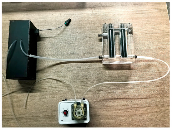
Figure 1.
Prototype of spectrometer prototype.
The light source component adopts a tungsten lamp full-spectrum light source with a wavelength range of 254–1275 nm, which is combined with a condenser to achieve beam collimation output. A total of 1920 spectral data can be obtained. The active cooling fan with a working voltage of 5 V and an air volume of 0.6 CFM is integrated on the back of the light source, which can control the working temperature of the light source at 45 ± 2 °C, effectively suppress thermal radiation noise, avoid detection errors caused by temperature changes, and ensure stable operation of the light source. Finally, the spectral data is transmitted to the host through the type-B interface on the spectrometer, and a water quality estimation model is constructed using machine learning algorithms to achieve accurate detection of water quality.
2.2. Experimental Design
Prepare 50 mL of potassium nitrate (Sinopharm Chemical Reagent Co., Ltd., Shanghai, China) solutions at concentrations ranging from 0 to 1 mol/L, with specific increments of 0, 0.02, 0.04, 0.06, 0.08, 0.1, 0.16, 0.2, 0.24, 0.28, 0.3, 0.36, 0.4, 0.44, 0.48, 0.5, 0.56, 0.6, 0.64, 0.68, 0.7, 0.76, 0.78, 0.8, 0.86, 0.9, 0.94, 0.96, and 1 mol/L using analytical-grade potassium nitrate. Similarly, prepare 50 mL of ammonium chloride (Sinopharm Chemical Reagent Co.Ltd., Shanghai, China) solutions at concentrations of 0, 0.02, 0.04, 0.06, 0.08, 0.1, 0.16, 0.2, 0.24, 0.28, 0.3, 0.36, 0.4, 0.44, 0.48, 0.5, 0.56, 0.6, 0.64, 0.68, 0.7, and 0.76 mol/L. Store the ammonium chloride solutions at concentrations of 0.78, 0.8, 0.86, 0.9, 0.94, and 1 mol/L in 50 mL brown centrifuge tubes.
Using a peristaltic pump, sequentially extract solutions of different concentrations (from low to high) and measure the spectral intensity (254–1275 nm) of a tungsten lamp (Ulode (Digital), model DivjAtnjw, Shanghai INESA(Group) Co., Ltd., Shanghai, China) passing through a quartz flow colorimetric dish (250 µL, optical path 10 mm) using a spectrometer according to the concentration order in Table 1. To eliminate errors caused by the equipment, the spectral intensity of the solutions was measured in reverse order (from high to low) on the second day.

Table 1.
Detection sequence of NH4 and NO3 different concentrations.
On the third day, reprepare 50 mL of potassium nitrate solutions at concentrations of 0, 0.12, 0.14, 0.18, 0.22, 0.26, 0.32, 0.34, 0.38, 0.42, 0.46, 0.52, 0.54, 0.58, 0.6, 0.62, 0.66, 0.72, 0.74, and 0.82 mol/L, and reprepare 50 mL of ammonium chloride solutions at concentrations of 0, 0.12, 0.14, 0.18, 0.22, 0.26, 0.32, 0.34, 0.38, 0.42, 0.46, 0.52, 0.54, 0.58, 0.62, 0.66, 0.72, 0.74, 0.82, 0.84, and 0.88 mol/L. On the fourth day, measure the spectral intensity of the two solutions in reverse order. This process yielded 96 spectral data sets for potassium nitrate solutions and 99 spectral data sets for ammonium chloride solutions.
2.3. Data Analysis Methods
The obtained spectral data were preprocessed using methods such as multiple scattering correction (MSC), Savitzky–Golay filtering (SG), and standardization (SS) to enhance the usability of the spectral data and improve the predictive capability of the analysis model.
Estimation methods for potassium nitrate and ammonium chloride content were established using SVM-MLP, SVR, RF, RF-Lasso, and PLSR in Python 3.9. SVR, MLP, RF, Lasso, and PLSR were based on the sklearn library (Version 1.5.1); the SVM-MLP algorithm was combined with the sequential method in TensorFlow (Version 2.10.0). The accuracy of the model was evaluated using mean absolute error (MAE), root mean square error (RMSE), mean square error (MSE), and coefficient of determination (R2).
3. Results
3.1. Correlation Analysis Between Nitrogen Indicators and Spectral Bands
The variation of nitrogen index light intensity with wavelength of all samlpes is shown in Figure 2. The main variation bands of NH4+ and NO3− are 254–550 nm and 950–1275 nm.
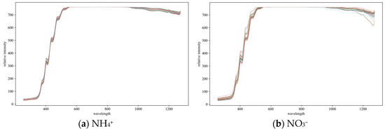
Figure 2.
Intensity curve of (a) NH4+ and (b) NO3−.
The correlation between nitrogen indicators and light intensity in different bands is shown in Figure 3. From Figure 3a, it can be seen that the correlation coefficient between NH4+ and light intensity in different bands ranges from −0.48 to 0.24. The bands with p-values less than 0.05 are mainly concentrated in 365–377 nm, 395–420 nm, 588–608 nm, 669–687 nm, 690–699 nm, 702 nm, 715 nm, 742 nm, 756–780 nm, 802–817 nm, 827–837 nm, 860–950 nm, and 1186–1275 nm, totaling 404 characteristic wavelength points; from Figure 3b, it can be seen that the correlation coefficient between NO3− and light intensity in different bands ranges from −0.43 to 0.19. The bands with p-values less than 0.05 are mainly concentrated in 619–701 nm, 705 nm, 788–790 nm, 793 nm, 794 nm, 804–807 nm, 816–819 nm, 826–827 nm, 836–846 nm, 858–864 nm, and 1037–1275 nm, totaling 454 characteristic wavelength points.
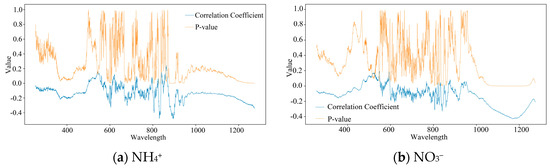
Figure 3.
Correlation between different wavelength light intensity and (a) NH4+ and (b) NO3− content.
3.2. Comparison of Full Band Raw Data Models and Spectral Screening Results
3.2.1. PCA Results
From Figure 4, it can be seen that the PCA of NH4+ spectra explains 67.11% and 30.26% of the data changes in the first and second principal axes, totaling 97.37%. The samples are mainly distributed in three concentrated areas (red circles in Figure 4a), with significant differences between the areas. The PCA of NO3− spectra explained 76.50% and 19.76% of the data changes in the first and second principal axes, totaling 96.26%. The samples were mainly distributed in three concentrated small areas (green circles in Figure 4b), with some differences between the areas.
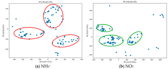
Figure 4.
PCA results of full band light intensity. The red circle represents the NH4+ sample aggregation area, and the green circle represents the NO3− sample aggregation area.
3.2.2. Analysis of Full Band Modeling Results
The prediction and evaluation results of the full band raw spectral data model for each water quality indicator are shown in Table 2. It can be seen that for NH4+, the PLSR model has the best prediction performance, with R2, MSE, RMSE, MAE, and Time of 0.8584, 0.0098, 0.0991, 0.0818, and 0.0307 s, respectively. The SVM-MLP and SVR algorithms are relatively poor. For NO3−, the PLSR model has the best prediction performance, with R2, MSE, RMSE, MAE, and time of 0.7376, 0.0252, 0.1589, 0.1313, and 0.0203 s, respectively. The SVM-MLP and SVR algorithms are relatively poor. The prediction results of 1DCNN for both indicators are not ideal.
Table 2.
Full band results under different models.
3.2.3. Selecting 1000 Main Bands for Modeling Result Analysis
The model prediction and evaluation results of the full band original spectral data of various water quality indicators after PCA dimensionality reduction to 1000 characteristic bands are shown in Table 3. From Table 3, it can be seen that for NH4+, the PLSR model has the best prediction performance, with R2, MSE, RMSE, MAE, and Time of 0.8428, 0.0109, 0.1045, 0.0899, and 0.021, respectively. The SVR algorithm is relatively poor. For NO3−, the PLSR model has the best prediction performance, with R2, MSE, RMSE, MAE, and time of 0.7243, 0.0265, 0.1629, 0.1337, and 0.0324 s, respectively. The SVR algorithm is relatively poor. The prediction results of 1DCNN for the two indicators are relatively good, with R2 values of 0.7429 and 0.6935 for NH4+ and NO3−, respectively.
Table 3.
Results of 1000 bands under different models.
3.2.4. Selecting 400 Main Bands for Modeling Result Analysis
The model prediction and evaluation results of the full band original spectral data of various water quality indicators after PCA dimensionality reduction to 400 characteristic bands are shown in Table 4. From Table 4, it can be seen that for NH4+, the SVM-MLP model has the best prediction performance, with R2, MSE, RMSE, MAE, and Time of 0.8726, 0.0088, 0.094, 0.0754, and 0.2111 s, respectively. The SVR algorithm is relatively poor. For NO3−, the 1DCNN model has the best prediction performance, with R2, MSE, RMSE, MAE, and Time of 0.7462, 0.0244, 0.1563, 0.1346, and 310.2073 s, respectively. The SVR algorithm is relatively poor. The prediction results of 1DCNN for the two indicators are relatively good, with R2 values of 0.7483 and 0.7462 for NH4+ and NO3−, respectively.
Table 4.
Results of 400 band models under different models.
3.3. Comparison of Spectral Models Under Different Preprocessing Methods
3.3.1. PCA Results After Preprocessing Using Three Methods
- (1)
- MSC. From Figure 5, it can be seen that the PCA of NH4+ spectra explains 51.20% and 45.75% of the data changes in the first and second principal axes, totaling 96.95%. The samples are mainly distributed in three concentrated areas (red circles in Figure 5a), with significant differences between the areas. The PCA of NO3− spectra explained 80.70% and 14.67% of the data changes in the first and second principal axes, totaling 95.37%. The samples were mainly distributed in three concentrated small areas (green circles in Figure 5b), with some differences between the areas.
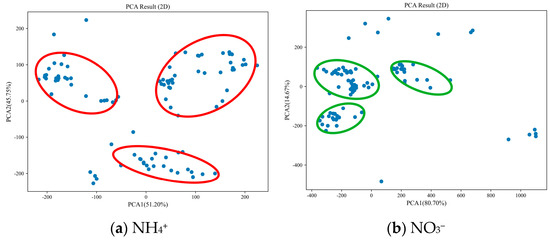 Figure 5. PCA results of sample data processed by MSC. The red circle represents the NH4+ sample aggregation area, and the green circle represents the NO3− sample aggregation area.
- (2)
- SG. From Figure 6, it can be seen that the PCA of NH4+ spectra explains 61.76% and 30.28% of the data changes in the first and second principal axes, totaling 92.04%. The samples are mainly distributed in three concentrated areas (red circles in Figure 6a), with significant differences between the areas. The PCA of NO3− spectra explained 76.51% and 19.76% of the data changes in the first and second principal axes, totaling 96.27%. The samples were mainly distributed in three concentrated small areas (green circles in Figure 6b), with some differences between the areas.
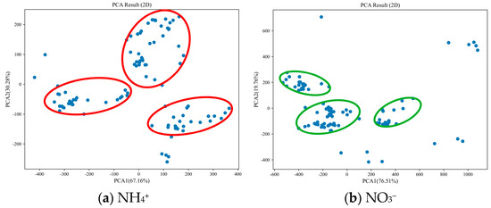 Figure 6. PCA results of sample data processed by SG. The red circle represents the NH4+ sample aggregation area, and the green circle represents the NO3− sample aggregation area.
- (3)
- SS. From Figure 7, it is evident that the PCA of NH4+ spectra accounts for 80.63% and 14.71% of the data variability along the first and second principal axes, respectively, summing up to 95.34%. The samples are predominantly clustered in three distinct regions (highlighted by red circles in Figure 7a), with notable differences among these areas. Similarly, the PCA of NO3− spectra explains 51.20% and 45.75% of the data variability along the first and second principal axes, respectively, totaling 96.95%. The samples are primarily concentrated in three small, distinct regions (indicated by green circles in Figure 7b), with some discernible differences among these areas.
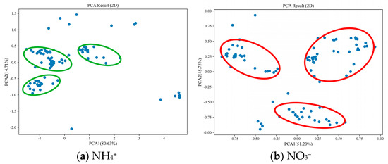 Figure 7. PCA results of sample data processed by SS. The red circle represents the NH4+ sample aggregation area, and the green circle represents the NO3− sample aggregation area.
3.3.2. Spectral Model Results After MSC Processing
The prediction and evaluation results of the MSC spectral full band model for various water quality indicators are shown in Table 5. From Table 5, it can be seen that for NH4+, the PLSR model has the best prediction performance, with R2, MSE, RMSE, MAE, and Time of 0.7735, 0.0157, 0.1254, 0.1089, and 0.0374 s, respectively. The SVR algorithm is relatively poor. For NO3−, the 1DCNN model has the best prediction performance, with R2, MSE, RMSE, MAE, and Time of 0.6425, 0.0344, 0.1855, 0.148, and 290.132 s, respectively. The SVR algorithm is relatively poor.
Table 5.
Results of spectral full band under different models processed by MSC.
The model prediction and evaluation results of MSC spectral data for various water quality indicators after PCA dimensionality reduction to 1000 characteristic bands are shown in Table 6. From Table 6, it can be seen that for NH4+, the SVM-MLP model has the best prediction performance, with R2, MSE, RMSE, MAE, and Time of 0.8263, 0.0121, 0.1098, 0.0932, and 0.4056 s, respectively. The SVR algorithm is relatively poor. For NO3−, the SVM-MLP model has the best prediction performance, with R2, MSE, RMSE, MAE, and Time of 0.6068, 0.0378, 0.1945, 0.1639, and 0.3851 s, respectively. The SVR algorithm is relatively poor. The prediction results for the two indicators SVM-ML are relatively good, with R2 values of 0.8263 and 0.6068 for NH4+ and NO3−, respectively.
Table 6.
Results of spectral 1000 bands under different models processed by MSC.
The model prediction and evaluation results of MSC spectral data for various water quality indicators after PCA dimensionality reduction to 400 characteristic bands are shown in Table 7. From Table 7, it can be seen that for NH4+, the SVM-MLP model has the best prediction performance, with R2, MSE, RMSE, MAE, and Time of 0.7754, 0.0156, 0.1249, 0.1018, and 0.165 s, respectively. The SVR algorithm is relatively poor. For NO3−, the SVM-MLP model has the best prediction performance, with R2, MSE, RMSE, MAE, and Time of 0.6465, 0.034, 0.1844, 0.1495, and 0.1513 s, respectively. The SVR algorithm is relatively poor. The prediction results for the two indicators SVM-MLP are relatively good, with R2 values of 0.7754 and 0.6465 for NH4+ and NO3−, respectively.
Table 7.
Results of spectral 400 bands under different models processed by MSC.
3.3.3. Spectral Model Results After SG Processing
The prediction and evaluation results of the SG spectral full band model for various water quality indicators are shown in Table 8. From Table 8, it can be seen that for NH4+, the PLSR model has the best prediction performance, with R2, MSE, RMSE, MAE, and Time of 0.8099, 0.0132, 0.1149, 0.0937, and 0.024 s, respectively. The SVM-MLP and SVR algorithms are relatively poor. For NO3−, the PLSR model has the best prediction performance, with R2, MSE, RMSE, MAE, and Time of 0.7136, 0.0276, 0.166, 0.1394, and 0.0202 s, respectively. The SVM-MLP and SVR algorithms are relatively poor. The prediction results for the two indicators PLSR are relatively good, with R2 values of 0.8099 and 0.7136 for NH4+ and NO3−, respectively.
Table 8.
Results of spectral full band under different models processed by SG.
The model prediction and evaluation results of SG spectral data for various water quality indicators after PCA dimensionality reduction to 1000 characteristic bands are shown in Table 9. From Table 9, it can be seen that for NH4+, the CAS-PLSR model has the best prediction performance, with R2, MSE, RMSE, MAE, and Time of 0.7904, 0.0145, 0.1206, 0.0911, and 18.7946 s, respectively. The SVR algorithm is relatively poor. For NO3−, the PLSR model has the best prediction performance, with R2, MSE, RMSE, MAE, and Time of 0.7173, 0.0272, 0.1649, 0.1382, and 0.0204 s, respectively. The SVR algorithm is relatively poor. With the dimensionality reduction of SG spectral data to 1000 feature bands through PCA, the prediction performance of SVM-MLP model has significantly improved.
Table 9.
Results of spectral 1000 bands under different models processed by SG.
The model prediction and evaluation results of SG spectral data for various water quality indicators after PCA dimensionality reduction to 400 characteristic bands are shown in Table 10. From Table 10, it can be seen that for NH4+, the CAS-PLSR model has the best prediction performance, with R2, MSE, RMSE, MAE, and Time of 0.797, 0.0141, 0.1187, 0.0897, and 11.4601 s, respectively. The SVM-MLP and SVR algorithms are relatively poor. For NO3−, the CAS-PLSR model has the best prediction performance, with R2, MSE, RMSE, MAE, and Time of 0.6332, 0.0353, 0.1879, 0.141, and 11.3003 s, respectively. The prediction results for the two indicators CAS-PLSR are relatively good, with R2 values of 0.797 and 0.6332 for NH4+ and NO3−, respectively.
Table 10.
Results of spectral 400 bands under different models processed by SG.
3.3.4. Spectral Model Results After SS Processing
The prediction and evaluation results of the SS spectral full band model for various water quality indicators are shown in Table 11. From Table 11, it can be seen that for NH4+, the PLSR model has the best prediction performance, with R2, MSE, RMSE, MAE, and Time of 0.7684, 0.0161, 0.1268, 0.1095, and 0.038 s, respectively. For NO3−, the 1DCNN model has the best prediction performance, with R2, MSE, RMSE, MAE, and Time of 0.7758, 0.0216, 0.1469, 0.1128, and 295.2939 s, respectively.
Table 11.
Results of spectral full band under different models processed by SS.
The model prediction and evaluation results of the SS spectral data of various water quality indicators after PCA dimensionality reduction to 1000 characteristic bands are shown in Table 12. From Table 12, it can be seen that for NH4+, the SVR model has the best prediction performance, with R2, MSE, RMSE, MAE, and Time of 0.7303, 0.0187, 0.1368, 0.1119, and 0.004 s, respectively. The SVM-MLP algorithm is relatively poor. For NO3−, the PLSR SVR model has the best prediction performance, with R2, MSE, RMSE, MAE, and Time of 0.6394, 0.0347, 0.1863, 0.1552, and 0.005 s, respectively. The prediction results for the two indicators SVR are better, with R2 values of 0.7303 and 0.6394 for NH4+ and NO3−, respectively.
Table 12.
Results of spectral 1000 bands under different models processed by SS.
The model prediction and evaluation results of SS spectral data for various water quality indicators after PCA dimensionality reduction to 400 characteristic bands are shown in Table 13. From Table 13, it can be seen that for NH4+, the SVM-MLP model has the best prediction performance, with R2, MSE, RMSE, MAE, and Time of 0.8876, 0.00478, 0.0883, 0.0683, and 0.1869 s, respectively. For NO3−, the 1DCNN model has the best prediction performance, with R2, MSE, RMSE, MAE, and Time of 0.5619, 0.0422, 0.2053, 0.1475, and 303.5223 s, respectively. From the comparison of Table 12 and Table 13, it can be seen that feature dimensionality reduction has a significant impact on model performance. Appropriate dimensionality reduction can remove redundant information, improving the prediction accuracy and generalization ability of the model.
Table 13.
Results of spectral 400 bands under different models processed by SS.
3.4. Comparison Between the Predicted and Measured Values of the Optimal Model
The optimal model for predicting ammonium chloride is the SVM-MLP model used to reduce the dimensionality of spectral data to 400 characteristic bands after SS processing. The comparison between the predicted values and the measured values is shown in Figure 8. The optimal model for predicting potassium nitrate is the 1DCNN model used for the full band spectral data after SS processing. The comparison results between the predicted values and the measured values, as well as the loss curve during the training process, are shown in Figure 9.
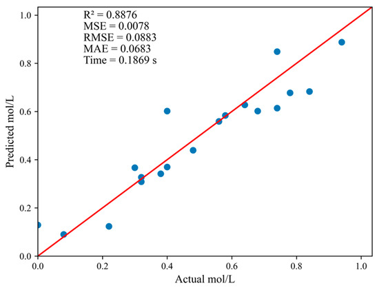
Figure 8.
The comparison between the predicted values and the measured values of NH4+ under SVM-MLP model with 400 bands processed by SS.
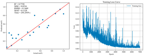
Figure 9.
The comparison between the predicted values and the measured values of NO3− under 1DCNN model with full band processed by SS.
4. Discussion
4.1. Water Quality Indicators Are Closely Related to Different Spectral Bands
Recent progress in UV-Vis spectroscopy has corroborated comparable absorption traits for nitrogen species under controlled conditions [27]. Taking the wavelength range of 365–377 nm as an illustration, NH4+ exhibits a notable correlation with light intensity. The underlying mechanism stems from the fact that the light energy in this range closely aligns with the energy necessary for the vibration or electronic transition of specific chemical bonds in NH4+, thereby enhancing absorption or scattering phenomena. During water’s phase transition, the formation of hydrogen bonds releases energy (ranging from approximately 12.81 to 69.69 kJ/mol). The wavelength range of photons corresponding to these energies is highly correlated with the experimentally observed anomalous infrared radiation, such as in the 8–14 µm and 1–4 µm ranges. For instance, the energy released from the formation of a single hydrogen bond (12.81 kJ·mol−1) corresponds to wavelengths of 8–14 µm, while the energy from multiple hydrogen bonds (35–69 kJ/mol) aligns with shorter wavelengths (1–4 µm). This mechanism bears a resemblance to the vibrational energy of the N-H bond in NH4+, where vibrational transitions may occur through a comparable process of photon energy release [28]. Molecular dynamics simulations have further elucidated the quantum mechanical foundations of these interactions [29]. The correlation of NO3− within the wavelength range of 619–701 nm is attributed to its unique ion structure and electron cloud distribution characteristics. In the ammonia oxidation reaction, the generation of NO3− involves a complex electron transfer process. For example, during the oxidation of NH3 to form HNO intermediates, the conjugated structure (planar triangle) of NO3− imparts symmetry to its electron cloud distribution, potentially leading to characteristic absorption in the visible light band (such as 619–701 nm) [30].
4.2. Impact of PCA Dimensionality Reduction on Model Accuracy
In the scenario of modeling using full band raw data, the PLSR model demonstrates good accuracy for predicting NH4+ and NO3− [31]. This is primarily due to PLSR’s proficiency in effectively managing the correlation among multiple variables. When dealing with high-dimensional spectral data, PLSR can comprehensively consider information from various bands and establish a stable relationship with water quality indicators. The superiority of PLSR in handling collinear spectral variables has been consistently validated across multiple studies [32].
Conversely, the 1DCNN model struggles with full band raw data. The raw spectral data not only has a high dimensionality but also contains significant noise, making it challenging for the 1DCNN model to accurately extract meaningful feature information, thus impacting its prediction performance. Deep learning models often require meticulous architecture design to tackle the challenges posed by spectral noise [33].
For NH4+, as the number of bands decreases, the model’s accuracy diminishes. This decline can be attributed to the fact that full band spectral data, while rich in information, may also contain redundant and noisy data. Lee et al. [34] suggested that band selection should prioritize regions with high signal-to-noise ratio and chemical specificity.
Following PCA dimensionality reduction, the data dimension is significantly reduced, redundant information is effectively eliminated [35], and the 1DCNN model can concentrate more on learning key features, leading to enhanced prediction performance. Karpagalakshmi et al. [36] proved that the PCA-RF model outperformed conventional machine learning approaches, achieving a high R-squared score of 0.95. This underscores that reasonable data dimensionality reduction can optimize the model’s training and prediction processes when dealing with high-dimensional spectral data. However, it is important to note that PCA dimensionality reduction inevitably leads to the loss of some valuable information while reducing data dimensionality. For instance, some spectral information that is weakly correlated with water quality indicators but may be crucial under specific conditions may be lost during the dimensionality reduction process. Nonlinear dimensionality reduction techniques may preserve more spectral information than PCA [37]. Therefore, in practical applications, it is essential to select spectral bands judiciously based on data characteristics and research objectives to strike a balance between model accuracy and computational efficiency.
4.3. Impact of Data Preprocessing on Model Accuracy
Data preprocessing is a pivotal factor that significantly influences the accuracy of predictive models [18]. Rinnan et al. [38] highlighted that MSC enhances data quality by aligning each spectrum to a reference through linear regression, thereby mitigating scattering effects. In our study, following MSC processing, PCA of ammonium chloride and potassium nitrate spectra revealed improvements in data interpretability and sample distribution, leading to enhanced predictive performance for certain models. This underscores the beneficial role of MSC in refining spectral data structure. Savitzky and Golay [39] demonstrated that the SG filter preserves the inherent signal shape while effectively suppressing high-frequency noise. Our experimental results indicate that SG processing improves the predictive performance of some models, particularly those that are noise-sensitive, emphasizing the importance of SG filtering in enhancing data quality. Barnes et al. [40] introduced the SNV transformation, which normalizes spectra on a row-wise basis to eliminate multiple interferences. SNV processing notably improved model prediction accuracy in specific scenarios, such as when using the SVM-MLP model for NH4+ with dimensionality reduced to 400 feature bands, and the 1DCNN model for NO3− across the entire spectral band. For full band spectral data of NH4+, after SNV processing, the PLSR model achieved an R2 of 0.7684 and an RMSE of 0.1268, indicating that different preprocessing methods can lead to subtle differences in model accuracy.
Combining multiple preprocessing methods is also a viable approach. Engel et al. [41] emphasized that the selection and sequence of preprocessing steps should be tailored to the specific spectral characteristics and analytical objectives. For spectral data exhibiting severe scattering, baseline drift, and significant noise interference, it is advisable to first apply MSC to correct scattering effects, followed by SG filtering to remove noise, and finally standardize the data using SNV processing. This comprehensive approach improves data quality and optimizes model performance across various aspects. Notably, there are considerable differences in the prediction accuracy of multiple models for NH4+ and NO3− in our study. However, the SVM-MLP and SVR algorithms exhibited poor performance in predicting these two indicators. Wold et al. [42] pointed out that PLSR excels in managing collinearity by projecting variables into latent structures. The SVM-MLP yielded R2 values of −6.8377 for NH4+ and −0.0230 for NO3−, indicating fundamental differences in the ability of various models to process spectral data and fit water quality indicators [43,44]. This disparity in accuracy primarily stems from the algorithmic principles and model structures [45]. PLSR, based on principal component regression, effectively extracts main components in spectral data, reduces multicollinearity among variables, and establishes a more accurate prediction model. In contrast, when dealing with high-dimensional and complex spectral data, SVM-MLP and SVR may have structural limitations, making it challenging to accurately capture the intricate nonlinear relationships between water quality indicators and spectral features, thus resulting in lower prediction accuracy.
4.4. Research Shortcomings and Future Research Directions
The findings of this research hold significant potential for wide-ranging applications. By leveraging the optimal model and spectral processing technique identified in this study, along with automated spectral monitoring equipment, it is feasible to establish a real-time, efficient nitrogen monitoring system for drinking water sources. The integration of portable spectrometers with edge computing devices now facilitates the deployment of field-ready solutions [46]. Nevertheless, real-world water bodies are considerably more complex than experimental solution systems, and the presence of suspended solids can introduce spectral interference [47,48]. To address this, Li et al. [49] suggested incorporating environmental variability into training datasets to bolster model generalizability. Given the limited sample size in the current study, further expansion of the sample size is imperative for the practical implementation of these research outcomes.
Rinnan et al. [50] underscored the importance of increasing sample heterogeneity to enhance model robustness against real-world variability. To this end, it is necessary to collect a substantial number of actual water samples under diverse environmental conditions, construct a data set encompassing multiple interfering factors, and subsequently train and validate the model. Valladares-Castellanos et al. [51] combined machine learning and spatial extrapolation to enhance ES modeling in data-scarce contexts. Xiao et al. [52] proposed a cross-basin machine learning model, the modeling strategy of which is better than a single basin machine learning model and grouped basin machine learning model. Moreover, there is a need to delve deeper into advanced data processing techniques and modeling approaches, such as convolutional neural networks (CNN), recurrent neural networks (RNN), and their variants like LSTM and GRU, within the realm of deep learning. These techniques are anticipated to enhance the accuracy and stability of water quality index spectral estimation models. Notably, transformer-based architectures have demonstrated remarkable success in spectral sequence modeling [53].
Furthermore, by integrating data from additional sensors, including temperature sensors, pH sensors, and dissolved oxygen sensors, multi-source data fusion can be achieved. This approach allows for a comprehensive analysis of the impact of multi-source data on water quality index estimation, thereby providing a more holistic representation of the true state of the water body and improving the model’s reliability and adaptability. By combining multispectral remote sensing images from unmanned aerial vehicles (UAVs) with artificial intelligence (AI) learning algorithms, including random forest (RF), gradient boosting regression tree (GBRT), partial least squares (PLS), and support vector machine (SVM), a water quality parameter (WQP) monitoring technology suitable for coastal aquaculture waters is established [54]. We are also using UAVs to collect water samples (Figure 10).
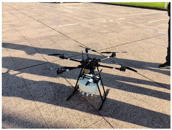
Figure 10.
Drones equipped with water sample collectors.
5. Conclusions
In this study, we developed a portable spectral detector designed for rapid on-site detection of water quality. By utilizing 0–1 mol·L−1 solutions of ammonium chloride and potassium nitrate, we constructed a water quality detection model. Our findings indicate that NH4+ and NO3− exhibit notable spectral changes within the transition band between ultraviolet and visible light, and the transition between near-infrared and mid infrared in the infrared region. When modeling raw data across all bands, the PLSR model demonstrated superior performance in predicting NH4+ and NO3−. For NH4+, the spectral data was reduced to 400 feature bands after applying SS processing by PCA dimensionality reduction, and the SVM-MLP model yielded the best prediction results. In the case of NO3−, the 1DCNN model exhibited relatively ideal prediction performance when utilizing the entire band after SS processing. These results clearly highlight the existence of a specific adaptation relationship between different pretreatment methods, water quality indicators, and modeling algorithms. In practical applications, it is crucial to select the most appropriate combination of pretreatment and modeling techniques based on the specific context to achieve optimal prediction outcomes.
Author Contributions
Conceptualization, B.Z.; methodology, H.L. and R.C.; software, H.L. and M.W.; formal analysis, H.L. and C.X.; investigation, H.L.,Y.H., and S.L.; resources, F.B.; data curation, H.Z. and D.S.; writing—original draft preparation, H.L.; writing—review and editing, D.S.; supervision, B.Z.; project administration, C.X. and M.W.; funding acquisition, B.Z. All authors have read and agreed to the published version of the manuscript.
Funding
This work was financially by Yafu Science and Technology projects plan of Jiangsu Vocational College of Agriculture and Forestry (2023kj05, 2024kj05), the Youth Support Project of Jiangsu Vocational College of Agriculture and Forestry (2022kj16, 2024kj44), and General Project of Basic Science (Natural Science) Research in Higher Education Institutions in Jiangsu Province (2024KJB210011).
Data Availability Statement
The raw data supporting the conclusions of this article will be made available by the authors on request.
Conflicts of Interest
The authors declare no conflicts of interest.
Abbreviations
The following abbreviations are used in this manuscript:
| MSC | Multiple Scattering Correction |
| SG | Savitzky–Golay Filtering |
| SS | Standardization |
| SVM | Support Vector Machine |
| MLP | Multilayer Perceptron |
| SVR | Support Vector Regression |
| RF | Random Forest |
| PLSR | Partial Least Squares Regression |
| PCA | Principal Component Analysis |
| RMSE | Root Mean Square Error |
| 1DCNN | 1D Convolutional Neural Network |
| UAVs | Unmanned Aerial Vehicles |
| LSTM | Long Short-Term Memory |
| KF | Kalman Filtering |
| CODMn | Permanganate index |
| SNV | Standard Normal Variate Transformation |
| XGBoost | eXtreme Gradient Boosting |
References
- Smith, J. Nitrogen dynamics in eutrophic freshwater systems. Environ. Sci. Technol. 2020, 12, 7213–7222. [Google Scholar]
- Johnson, M.; Lee, K. Challenges in environmental monitoring infrastructure development. Glob. Environ. Change 2018, 52, 54–63. [Google Scholar]
- Imaizumi, M. Time Series Analysis of Influence of Water Cycle on Nitrate Contamination in Miyako Island Ryukyu Limestone Aquifer. Water 2025, 18, 2723. [Google Scholar] [CrossRef]
- Mitchell, V.; Gong, J.; Moon, E.; Wu, W. Bushfire Impact on Drinking Water Distribution Networks and Investigation Methods: A Review. Water Resour. Res. 2025, 3, e2024WR038225. [Google Scholar] [CrossRef]
- Rogers, K.M.; Tschritter, C.; Bradshaw, D.; Abel, S.; Pannell, J.L.; Thern, J.; Heath, T.; Tio, P.; Liu, X.; Buckthought, L.; et al. A New Zealand freshwater nitrate data quality validation study using commercial laboratories and portable testing instruments. Chemosphere 2025, 381, 144472. [Google Scholar] [CrossRef]
- Zhang, X.; Ma, L.; Xu, Y. Design of Aquaculture Water Quality Monitoring System Based on Wireless Communication. In Proceedings of the International Conference on Information Control, Electrical Engineering and Rail Transit, Shanghai, China, 17–19 November 2023; Springer Nature: Singapore, 2025. [Google Scholar] [CrossRef]
- Huang, X.; Xiong, J.; Lin, H.; Pan, Z.; Wang, K.; Zhang, M.; Zhu, Z.; Ou, Y. Research on water quality detection integrating spectral analysis and automated control. Spectrochim. Acta Part A Mol. Biomol. Spectrosc. 2025, 339, 126260. [Google Scholar] [CrossRef] [PubMed]
- Xu, Z.; Li, X.; Cheng, W.; Zhao, G.; Tang, L.; Yang, Y.; Wu, Y.; Zhang, P.; Wang, Q. Data fusion strategy based on ultraviolet–visible spectra and near-infrared spectra for simultaneous and accurate determination of key parameters in surface water. Spectrochim. Acta Part A Mol. Biomol. Spectrosc. 2023, 302, 123007. [Google Scholar] [CrossRef]
- Liu, M. Application of fluorescence spectrum detection technology in COD detection of water quality. Hydro Sci. Cold Zone Eng. 2024, 10, 75–78. [Google Scholar] [CrossRef]
- Gao, B.-C.; Li, R.-R.; Montes, M.J.; Mccarthy, S.C. Combining Cirrus and Aerosol Corrections for Improved Reflectance Retrievals over Turbid Waters from Visible Infrared Imaging Radiometer Suite Data. Oceans 2025, 2, 28. [Google Scholar] [CrossRef]
- Thompson, R. Hyperspectral imaging for contaminant detection. Anal. Chem. 2019, 3, 2149–2157. [Google Scholar]
- Harvey, E.T.; Kratzer, S.; Philipson, P. Satellite-based water quality monitoring for improved spatial and temporal retrieval of chlorophyll-a in coastal waters. Remote Sens. Environ. 2015, 158, 417–430. [Google Scholar] [CrossRef]
- Wang, M.; Pang, C.; Shi, B.; Schang, C.; Nolan, M.; Poon, R.; Catsamas, S.; Zhu, W.; Mccarthy, D. A Low-Cost, Open-Source, 3D-Printed, Compact, In Situ, Automatic Water Sampler for Environmental Surveillance. ACS EST Water 2025, 7, 4067–4078. [Google Scholar] [CrossRef]
- Moon, J.; Jung, S.; Suh, S.; Pyo, J. Development of deep learning quantization framework for remote sensing edge device to estimate inland water quality in South Korea. Water Res. 2025, 283, 123760. [Google Scholar] [CrossRef]
- Obořilová, R.; Buzík, J.; Skládal, P.; Farka, Z.; Lacina, K. Portable turbidimetric device for in-time monitoring of bacterial contamination in drinking water. J. Water Process Eng. 2025, 74, 107832. [Google Scholar] [CrossRef]
- Jekel Könnel, E.; Nonno, S.D.; Ulber, R. Low-cost and easy-to-use: A portable photometer for simple and comprehensive analysis of critical water quality parameters. Microchem. J. 2025, 214, 113946. [Google Scholar] [CrossRef]
- Liu, G.; Gong, Y.; Zhang, H.; Liang, H. Infrared Spectral Noise Reduction Algorithm Based on Wavelet Transform Optimized EEMD Combined with SG. Infrared Technol. 2024, 12, 1453–1458. [Google Scholar]
- Li, K.; Guo, Y.; Zhong, H.; Jin, Y.; Li, B.; Fang, H.; Yao, L.; Zhao, C. Rapid Identification of Dendrobium Species Using Near-Infrared Hyperspectral Imaging Technology. Sensors 2025, 18, 5625. [Google Scholar] [CrossRef]
- Souza, L.L.D.; Candeias, D.N.C.; Moreira, E.D.T.; Diniz, P.H.G.D.; Springer, V.H.; Fernandes, D.D.D.S. UV–Vis spectralprint-based discrimination and quantification of sugar syrup adulteration in honey using the Successive Projections Algorithm (SPA) for variable selection. Chemom. Intell. Lab. Syst. 2025, 257, 105314. [Google Scholar] [CrossRef]
- Zhou, H.; Xu, H.; Long, L.; Ji, D.; Han, Y.; Ji, X.; Cui, Y. A Comparative Study of Hyperspectral Estimation Models for Total Phosphorus and Total Nitrogen in the Midstream of the Xiangxi River. China Rural. Water Hydropower 2024, 11, 125–132. [Google Scholar] [CrossRef]
- Gao, Z.; Wang, G.; Chen, J.; Fang, L.; Ren, S.; Yinglan, A.; Ji, S.; Liu, R.; Wang, Q. Kalman filtering assimilated machine learning methods significantly improve the prediction performance of water quality parameters. Ecol. Inform. 2025, 90, 103337. [Google Scholar] [CrossRef]
- Zhang, L. Deep learning for spectral analysis. IEEE Trans. Geosci. Remote Sens. 2021, 6, 5041–5052. [Google Scholar]
- Wei, Y.; Zhong, R.; Yang, Y. Groundwater Fluoride Prediction for Sustainable Water Management: A Comparative Evaluation of Machine Learning Approaches Enhanced by Satellite Embeddings. Sustainability 2025, 18, 8505. [Google Scholar] [CrossRef]
- Das, A. Surface water quality evaluation, apportionment of pollution sources and aptness testing for drinking using water quality indices and multivariate modelling in Baitarani River basin, Odisha. HydroResearch 2025, 8, 244–264. [Google Scholar] [CrossRef]
- Sattley, W.M.; Burchell, B.M.; Conrad, S.D.; Madigan, M.T. Design, Construction, and Application of an Inexpensive, High-Resolution Water Sampler. Water 2017, 8, 578. [Google Scholar] [CrossRef]
- Sánchez-Saquín, C.H.; Soto-Cajiga, J.A.; Barrera-Fernández, J.M.; Gómez-Hernández, A.; Rodríguez-Olivares, N.A. Identification, Control, and Characterization of Peristaltic Pumps in Hemodialysis Machines. Appl. Syst. Innov. 2025, 2, 44. [Google Scholar] [CrossRef]
- Brown, A. UV—Vis spectroscopy of nitrogen compounds. J. Phys. Chem. A 2021, 18, 3987–3995. [Google Scholar]
- Tatartchenko, V. Infrared radiation during phase transitions of water. J. Phys. Chem. B 2012, 12, 3726–3734. [Google Scholar]
- Schmidt, M. Quantum mechanical modeling of NH4+ spectra. J. Chem. Phys. 2023, 158, 4. [Google Scholar]
- Stagni, A. Experimental and kinetic modeling study of ammonia oxidation. React. Chem. Eng. 2020, 3, 456–467. [Google Scholar] [CrossRef]
- Liu, X.; Zhou, L.; Xia, X.; Han, R.; Lyu, Q.; Xie, R.; Yi, S. Predicting Citrus Leaf Nitrogen Content Based on Hybrid Bat Algorithm Optimized PLSR. J. Southwest Univ. (Nat. Sci. Ed.) 2025, 2, 160–170. [Google Scholar] [CrossRef]
- Puttipipatkajorn, A.; Puttipipatkajorn, A. Development of low-cost portable spectrometer equipped with 18-band spectral sensors using deep learning model for evaluating moisture content of rubber sheets. Smart Agric. Technol. 2024, 9, 100562. [Google Scholar] [CrossRef]
- Wong, C.; Gesmundo, A. Transfer Learning to Learn with Multitask Neural Model Search. arXiv 2017, arXiv:1710.10776. [Google Scholar] [CrossRef]
- Lee, L.C.; Liong, C.-Y.; Jemain, A.A. A contemporary review on Data Preprocessing (DP) practice strategy in ATR-FTIR spectrum. Chemom. Intell. Lab. Syst. 2017, 163, 64–75. [Google Scholar] [CrossRef]
- Pishini, K.; Abdolazimi, O.; Shishebori, D.; Rezaee, M.J.; Sepehrifar, M. Evaluating efficiency in water and sewerage services: An integrated DEA approach with DOE and PCA. Sci. Total Environ. 2025, 959, 178288. [Google Scholar] [CrossRef]
- Karpagalakshmi, R.C.; Selvam, P.; Sakthivel, S.; Kalaivanan, K.; Sharma, R.; Sungheetha, A.; Mahapatra, S. Analysis of Water Quality in Cauvery River by Using PCA with Various Classifications Technique. Procedia Comput. Sci. 2025, 258, 1391–1403. [Google Scholar] [CrossRef]
- Ivakhno, S.; Armstrong, J.D. Non-linear dimensionality reduction of signaling networks. BMC Syst. Biol. 2007, 1, 27. [Google Scholar] [CrossRef] [PubMed]
- Rinnan, A.; Van Den, B.F.; Engelsen, S.B. Review of the most common pre-processing techniques for Near-Infrared spectra. Trends Anal. Chem. 2009, 28, 1201–1222. [Google Scholar] [CrossRef]
- Savitzky, A.; Golay, M.J.E. Smoothing and Differentiation of Data by Simplified Least Squares Procedures. Anal. Chem. 1964, 8, 1627–1639. [Google Scholar] [CrossRef]
- Barnes, R.J.; Dhanoa, M.S.; Lister, S.J. Standard Normal Variate Transformation and De-trending of Near-Infrared Diffuse Reflectance Spectra. Appl. Spectrosc. 1989, 5, 772–777. [Google Scholar] [CrossRef]
- Engel, J.; Gerretzen, J.; Szymańska, E.; Jansen, J.J.; Downey, G.; Blanchet, L.; Buydens, L.M.C. Breaking with trends in pre-processing? TrAC Trends Anal. Chem. 2013, 50, 96–106. [Google Scholar] [CrossRef]
- Wold, S.; Sjöström, M.; Eriksson, L. PLS-regression: A basic tool of chemometrics. Chemom. Intell. Lab. Syst. 2001, 2, 109–130. [Google Scholar] [CrossRef]
- Wang, Y.; Wang, C.; Wang, H. Simulated Estimation of BOD Content in Water Bodies Based on PCA Transmission Spectrum Reconstruction With Noise Reduction. Spectrosc. Spectr. Anal. 2025, 2, 386–393. [Google Scholar]
- Xiao, M.; Zhu, Y.; Gao, W.; Zeng, Y.; Li, H.; Chen, S.; Liu, P.; Huang, H. Comparative Study of Water Quality Prediction Methods Based on Different Artificial Neural Network. Environ. Sci. 2024, 10, 5761–5767. [Google Scholar] [CrossRef]
- Sarpal, D.; Sinha, R.; Jha, M.; Tn, P. AgriWealth: IoT based farming system. Microprocess. Microsyst. 2022, 89, 104447. [Google Scholar] [CrossRef]
- Li, Y.; Guo, J.; Liu, G.; Zhang, J.; Guo, Z.; Wang, W. Design of high speed miniature spectrometer based on FPGA. Proc. SPIE 2024, 13070, 130700J. [Google Scholar] [CrossRef]
- Irwan, D.; Ibrahim, S.L.; Latif, S.D.; Winston, C.A.; Ahmed, A.N.; Sherif, M.; El-Shafie, A.H.; El-Shafie, A. River water quality monitoring using machine learning with multiple possible in-situ scenarios. Environ. Sustain. Indic. 2025, 26, 100620. [Google Scholar] [CrossRef]
- Clark, R.N.; Roush, T.L. Reflectance spectroscopy: Quantitative analysis techniques for remote sensing applications. J. Geophys. Res. Solid Earth 1984, B7, 6329–6340. [Google Scholar] [CrossRef]
- Li, F.L.; Chang, Q.R. Estimation of winter wheat leaf nitrogen content based on continuum removed spectra. J. Agric. Mach. 2017, 7, 174–179. [Google Scholar]
- Rinnan, S. Pre-processing in vibrational spectroscopy—When, why and how. Anal. Methods 2014, 18, 7124. [Google Scholar] [CrossRef] [PubMed]
- Valladares-Castellanos, M.; De Jesús Crespo, R.; Douthat, T. Using machine learning for long-term calibration and validation of water quality ecosystem service models in data-scarce regions. Sci. Total Environ. 2025, 1000, 180388. [Google Scholar] [CrossRef] [PubMed]
- Xiao, F.; Zhang, R.; Jian, Z.; Liu, W.; Sun, T.; Pang, W.; Han, L.; Qin, H. Using ensemble machine learning to predict and understand spatiotemporal water quality variations across diverse watersheds in coastal urbanized areas. Ecol. Indic. 2025, 178, 113976. [Google Scholar] [CrossRef]
- Chen, W.; Ren, T.; Zhao, C.; Wen, Y.; Gu, Y.; Zhou, M.; Wang, P. Transformer-Based Fast Mole Fraction of CO2 Retrievals from Satellite-Measured Spectra. J. Remote Sens. 2025, 5, 0470. [Google Scholar] [CrossRef]
- Li, W.; Ren, M.; Zhang, H.; Duan, Y.; Chen, D.; Li, S.; Xu, M.; Wang, L.; Yang, X. Estimation of water quality in coastal aquaculture waters using the combination of machine learning and unmanned aerial vehicle multispectral imagery. Aquaculture 2026, 611, 743002. [Google Scholar] [CrossRef]


Disclaimer/Publisher’s Note: The statements, opinions and data contained in all publications are solely those of the individual author(s) and contributor(s) and not of MDPI and/or the editor(s). MDPI and/or the editor(s) disclaim responsibility for any injury to people or property resulting from any ideas, methods, instructions or products referred to in the content. |
© 2025 by the authors. Licensee MDPI, Basel, Switzerland. This article is an open access article distributed under the terms and conditions of the Creative Commons Attribution (CC BY) license (https://creativecommons.org/licenses/by/4.0/).