TCN-Transformer-Based Risk Assessment Method for Power Flow and Voltage Limit Violations in Active Distribution Networks

Abstract

With the increasing penetration of renewable energy, traditional distribution network operation state assessment methods based on typical operating conditions are no longer applicable. It is urgent to conduct risk assessment research on the dynamic coupling characteristics of voltage, power flow, and distributed generation output after photovoltaic integration into active distribution networks. This paper first analyzes the spatiotemporal variation characteristics of power flow distribution and voltage fluctuations in active distribution networks, and proposes evaluation indicators for power flow and voltage over limit risks. Secondly, feature quantities related to the over limit risk assessment indicators are selected, and a distribution network over limit risk assessment method based on TCN-Transformer neural network architecture is proposed. Finally, based on the improved IEEE 33 node distribution network model, an active distribution network simulation model is built in Matlab (2023b), and a simulation dataset is constructed for multiple operating scenarios. On this basis, a comparative analysis of risk assessment examples for power flow and voltage exceeding limits is conducted, and the results verify the effectiveness and superiority of the proposed method.

1. Introduction

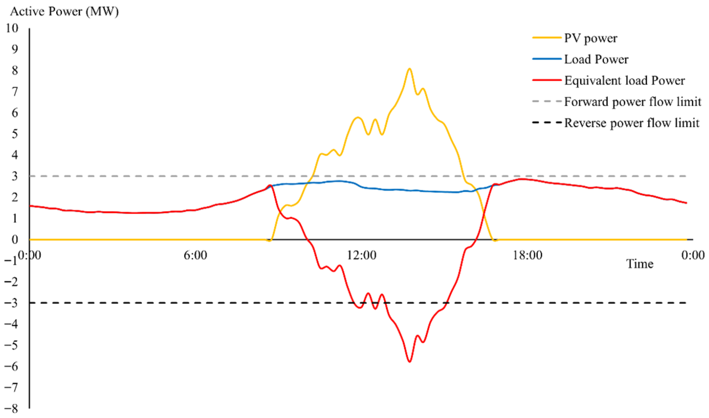
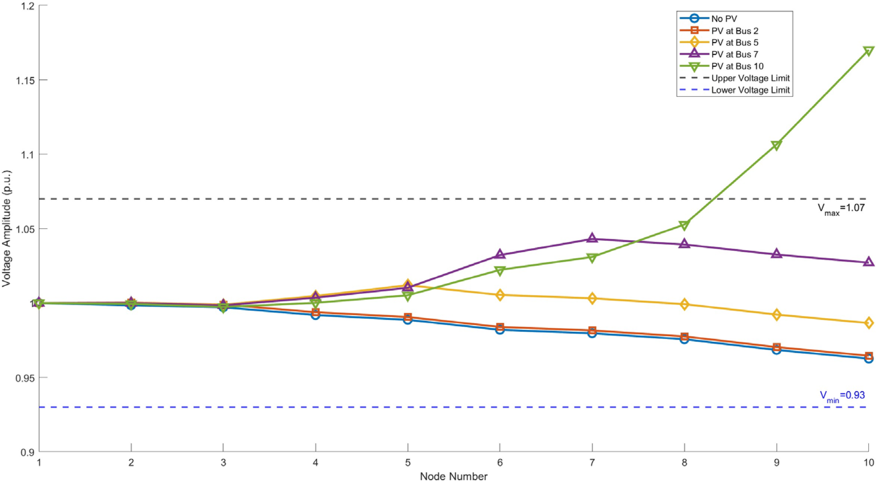
With the large-scale integration of distributed photovoltaics (PV), the power flow in active distribution networks exhibits bidirectional and stochastic characteristics. When distributed PV generation significantly exceeds local load demand and cannot be locally consumed, the risk of reverse power flow and subsequent limit violations surges dramatically. Concurrently, the risks of voltage exceeding upper limits during periods of high PV generation and dropping below lower limits during low generation periods become prominent, severely compromising user power quality. These operational challenges directly impact utility operations by increasing dispatch complexity, threatening grid reliability through potential protective device operations, and limiting PV hosting capacity due to conservative network constraints. There is an urgent need to assess power flow and voltage violation risks in active distribution networks, providing critical references for distribution network dispatch operations and distributed PV hosting capacity evaluation.

Existing research on risk assessment for distribution networks primarily focuses on two aspects: evaluation metrics and risk probability distributions. The work [1] proposed a voltage violation risk assessment index and classified the risk into low, medium, and high levels based on the index, enabling dynamic power flow-based risk warning. The work [2] designed a hierarchical risk assessment framework based on risk value theory, incorporating voltage violation indices. The work [3,4,5] introduced indices based on utility theory, event severity, and fuzzy cost, respectively. However, most of these studies rely on single-dimensional metrics focusing solely on either security or economy, lacking a universal and standardized index system. The works [6,7] employed probabilistic power flow models based on Copula theory or Monte Carlo simulation to quantify the risk of node voltage violation. The work [8,9] further employed stochastic power flow models to address uncertainties from both supply and demand sides, highlighting the limitations of traditional analytical methods in handling high-dimensional dynamic variations. Collectively, existing approaches lack an efficient and comprehensive framework for assessing risks under multi-scale spatiotemporal uncertainties, creating a clear gap that necessitates the adoption of data-driven artificial intelligence techniques.

With the increasing penetration of distributed generation and enhanced load uncertainty in distribution networks, deep learning-based prediction models for active distribution networks have become a core technology for dynamic risk assessment. The works [10,11] employed Long Short-Term Memory (LSTM) models to predict power system violation probabilities and violation risk indices. The work [12] utilized Gated Recurrent Units (GRU) integrated with meteorological data to achieve dynamic prediction of distributed PV output. However, it failed to account for the impact of dynamic load-side variations on the distribution network, making it difficult to meet the demands of dynamic risk assessment. Beyond classical LSTM and GRU, Temporal Convolutional Network (TCN) [12,13,14] offers advantages in parallel processing and capturing long-range temporal dependencies, proving effective in identifying periodic and sudden risks in distribution systems. The work [15,16] utilized TCN for load and renewable generation forecasting to support voltage assessment and flow risk analysis, though performance under imbalanced sample conditions remains a challenge. The work [17] proposed an integrated framework based on the Transformer model for predicting and risk-assessing the spatiotemporal distribution of heavy overloads in distribution networks under highly imbalanced and nonlinear data scenarios. The work [18] used the Transformer model for deterministic point prediction of power system risk assessment indices but did not provide a method for assessing violation risks. Notably, practical compliance with national standards [19] on voltage deviation requires interval-based prediction to quantify violation probabilities, calling for more informative and actionable risk evaluation methods.

To address this, the work [20] integrated temporal deep learning models with the Lower Upper Bound Estimation (LUBE) method [21]. This approach resolves the issue of interval prediction methods neglecting temporal dependencies, extending deterministic prediction models to provide a reference for dynamic assessment of power flow and voltage violations in distribution networks. Inspired by References [18,19,20,21], this paper addresses the power flow/voltage violation risks arising from high-penetration distributed PV integration into active distribution networks by constructing reasonable risk assessment indices combined with deep learning. On this basis, by analyzing the spatiotemporal characteristics of power flow/voltage in active distribution networks and constructing a modified IEEE 33-bus system for simulation experiments, the effectiveness of the proposed method is verified. The main innovations of this paper are as follows:

• To holistically evaluate violation risks caused by high-penetration distributed PV integration, this paper proposes the maximum positive/negative voltage deviation, and a composite power flow violation risk index.
• Considering the spatiotemporal characteristics of voltage and power flow in active distribution networks, a risk assessment model based on TCN-Transformer is proposed to further explore the correlation between the risk of voltage/power flow limit violation and related physical quantities in active distribution networks.
• Based on the physical significance of voltage and power flow violation risk indicators, different loss functions of neural network model are constructed to predict the numerical and interval values of power flow and voltage exceeding risk indicators, respectively, achieving accurate assessment of over limit risks in active distribution networks.

The paper is structured as follows: Section 1 outlines the research background and significance, and reviews the current state of research on power flow and voltage violations in distribution networks. Section 2 analyzes the spatiotemporal characteristics of power flow and voltage in active distribution networks, providing a basis for modeling. Section 3 elaborates on the proposed evaluation method, including indicators, models, and procedures. Section 4 presents case studies to assess power flow and voltage violation risks, demonstrating the superiority of the proposed approach. Section 5 summarizes the research findings and suggests directions for future work.

2. Analysis of Spatiotemporal Characteristics of Power Flow and Voltage in Active Distribution Networks

2.1. Spatiotemporal Characteristics of Power Flow in Active Distribution Networks

2.1.1. Temporal Characteristics of Power Flow in Active Distribution Networks

When distributed PV systems are integrated into the distribution network, let the load power be $P_L$ and the injected power from distributed PV be $P_{PV}$. The equivalent load power of the distribution network is then $P_{eq}=P_L-P_{PV}$. Both distributed PV output and load exhibit randomness and fluctuation. The fluctuation curves of PV output and load during a typical day are shown in Figure 1. During peak solar hours, PV generation significantly exceeds load demand ($P_{PV}>>P_L$), resulting in reverse power flow towards the main grid. This reverse flow may exceed the rated transmission capacity of distribution lines, creating a high risk of power flow violation. During night period with zero PV output ($P_{PV}=0$), the system reverts to a traditional grid structure where the main grid supplies the load. The magnitude of power flow varies with load fluctuations, and violations are less susceptible to occur under normal load conditions. During other Periods, PV generation and load consumption often achieve local balancing ($P_{PV}\approx P_L$). Power flow levels are generally low, making violations less likely.

2.1.2. Spatial Characteristics of Power Flow in Active Distribution Networks

In a feeder of the distribution network shown in Figure 2, the direction of the power flow is defined as positive from left to right. Among them, loads are connected at Buses 1–10, while PV systems are integrated at Buses 11–14 and sequentially connected to the distribution network at Buses 2, 5, 7, and 9. Due to distributed PV grid integration, reverse power flow occurs in branches where Branch 6–7 and Branch 9–10 are located, while upstream or middle sections of the line maintain forward power flow. The closer the PV integration bus is to the end of the feeder, the easier it is to form reverse power flow when the local load is less than PV output, potentially causing power flow violation risks.

2.2. Spatiotemporal Characteristics of Voltage in Active Distribution Networks

2.2.1. Temporal Characteristics of Voltage in Active Distribution Networks

Taking the single distribution line shown in Figure 3 as an example, the power flow direction from left to right is defined as positive, with line losses neglected. Before distributed PV integration, the voltage drop $\Delta U_k$ between Node k and Node k − 1 is:

$$\Delta U_k=U_k-U_{k-1}=-{\displaystyle \frac{{\displaystyle \sum _{m=i}^n{P}_m{R}_k+{\displaystyle \sum _{m=i}^n{Q}_m{X}_k}}}{U_{k-1}}}$$

(1)

where $P_m$ and $Q_m$ represent the active power and reactive power of the load at node $m$ ($m=1,2\dots ,n$); $n$ is the number of connected loads; $R_k$ and $X_k$ represent the resistance and reactance of the line between Node $k$ and Node $k-1$, respectively.

Therefore, the voltage magnitude $U_{k0}$ at Node $k$ is:

$$U_{k0}=U_0+{\displaystyle \sum _{i=1}^k\Delta U_i=U_0-{\displaystyle \sum _{i=1}^k\frac{{\displaystyle \sum _{m=i}^n{P}_m{R}_i+{\displaystyle \sum _{m=i}^n{Q}_m{X}_i}}}{U_{i-1}}}}$$

(2)

When a single distributed PV system with power $P_{pv}+j{Q}_{PV}$ is connected from Nodes k + 1 to n, the voltage magnitude $U_k$ at Node $k$ is:

$$U_k=U_0-{\displaystyle \sum _{i=1}^k\frac{({\displaystyle \sum _{m=i}^n{P}_m-P_{pv})R_i+({\displaystyle \sum _{m=i}^n{Q}_i-Q_{pv})X_i}}}{U_{i-1}}}$$

(3)

As derived from Equation (3), during the noon period, PV generation will also generate reactive power at a specific power factor, causing reactive power surplus at node $k$, i.e., ${\displaystyle \sum _{m=i}^n(Q_i-Q_{pv})}<0$, $U_k>U_0$. It leads to voltage progressively increasing from left to right, with the terminal node $n$’s voltage exceeding the upper limit becoming particularly prominent. During nighttime periods, PV generate neither active nor reactive power. When line length is excessive or loads are heavy, i.e., $U_k<U_0$, voltage progressively decreases from left to right, with the terminal Node $n$’s voltage exceeding the lower limit becoming particularly prominent. During other periods, voltage violation issues in the distribution network are less prominent.

2.2.2. Spatial Characteristics of Voltage in Active Distribution Networks

As indicated by Equation (3), the integration location of distributed PV also affects distribution network voltages. In the IEEE 10-bus system, the larger the access node number, the closer the PV access location is to the end of the feeder line. Connect the distributed PV systems to Buses 2, 5, 7, and 10, respectively, and simulate the voltage distribution of the nodes as shown in Figure 4.

As observed from Figure 4: When distributed PV systems of identical capacity are integrated at different locations, voltage profiles across nodes exhibit distinct variations; the voltage rise effect is negatively correlated with the electrical distance from the PV integration point to the feeder head. PV integration at the feeder end causes the most significant node voltage changes, easily causing voltages to exceed the upper limit; whereas PV integration closer to the feeder head has a relatively smaller impact on system voltage profiles.

3. Power Flow and Voltage Violation Risk Assessment Method for Distribution Networks Based on Transformer Model

Through the above analysis, it can be concluded that in order to evaluate the risk of power flow and voltage violation under spatiotemporal coupling, it is necessary to establish reasonable risk assessment indicators for distribution networks. Moreover, deep learning models can capture the spatiotemporal dependencies of generation-load fluctuations, laying the foundation for dynamic risk assessment. Therefore, this section develops a violation risk assessment method for distribution networks by proposing voltage and power flow risk indices and leveraging deep learning models.

3.1. Risk Assessment Indicators for Power Flow and Voltage Violation

3.1.1. Risk Assessment Indicators for Power Flow Violation

The existence of power flow violation risks is determined based on the thermal stability limit of lines. The power flow violation rate $S_V$ for the entire distribution network is represented by the ratio of the number of actual violation branches $I_n$ to the total number of branches $I_N$ in the distribution system:

$$S_V={\displaystyle \frac{I_n}{I_N}}\times 100\%$$

(4)

Moreover, the relationship between risks caused by power flow violations and problem severity is often nonlinear, and power flow violations often lead to an exponential increase in operational risks for the distribution network. Therefore, a power flow violation severity index $H_S$ is established based on a risk-preference utility function [22]:

$$H_S=e^{\Delta S_{\max }}-1$$

(5)

$$\Delta S_{max}=\max (S_i-S_C)$$

(6)

where $\Delta S_{max}$ denotes the maximum value of the branch power flow violation: $S_i$ denotes the apparent power of the line, and $S_C$ represents the maximum transmission capacity of the line.

By comprehensively considering both the extent and severity of power flow violations, the risk assessment indicator for power flow violation is yielded as $Risk$:

$$Risk=S_V\cdot H_S={\displaystyle \frac{I_n}{I_N}}\cdot \left(e^{\Delta S_{\max }}-1\right)\times 100\%$$

(7)

By identifying and analyzing the key characteristic factors that influence power flow limit violation risks, a predictive value for the risk assessment indicator Risk of future power flow limit violations is generated. This enables the evaluation of the future power flow violation risk in the distribution system.

3.1.2. Risk Assessment Indicators for Voltage Violation Risk

The voltage violation risk is quantified by employing the maximum positive voltage deviation $\Delta U_{\max }^{+}$ and the maximum negative voltage deviation $\Delta U_{\max }^{-}$ at each node in the distribution network:

$$\begin{array}{l}\Delta U_{\max }^{+}=\max \left\{\Delta U_i|\Delta U_i>0,i=1,2,\dots ,n\right\}\\ \Delta U_{\max }^{-}=\max \left\{\Delta U_i|\Delta U_i<0,i=1,2,\dots ,n\right\}\end{array}$$

(8)

where $\Delta U_i={\displaystyle \frac{U_i-U_N}{U_N}}$, $U_i$ denotes the voltage at Node $i$; $U_N$ refers to the rated voltage for the corresponding voltage level. All values are expressed in per-unit values.

By predicting the fluctuation range of $\Delta U_{\max }^{+}$ and $\Delta U_{\max }^{-}$, and comparing them with the voltage upper and lower bounds allowed by the national standard [19], the risk of voltage violation in the future of the distribution system can be evaluated.

3.2. TCN-Transformer-Based Model for Power Flow and Voltage Violation Risk Assessment

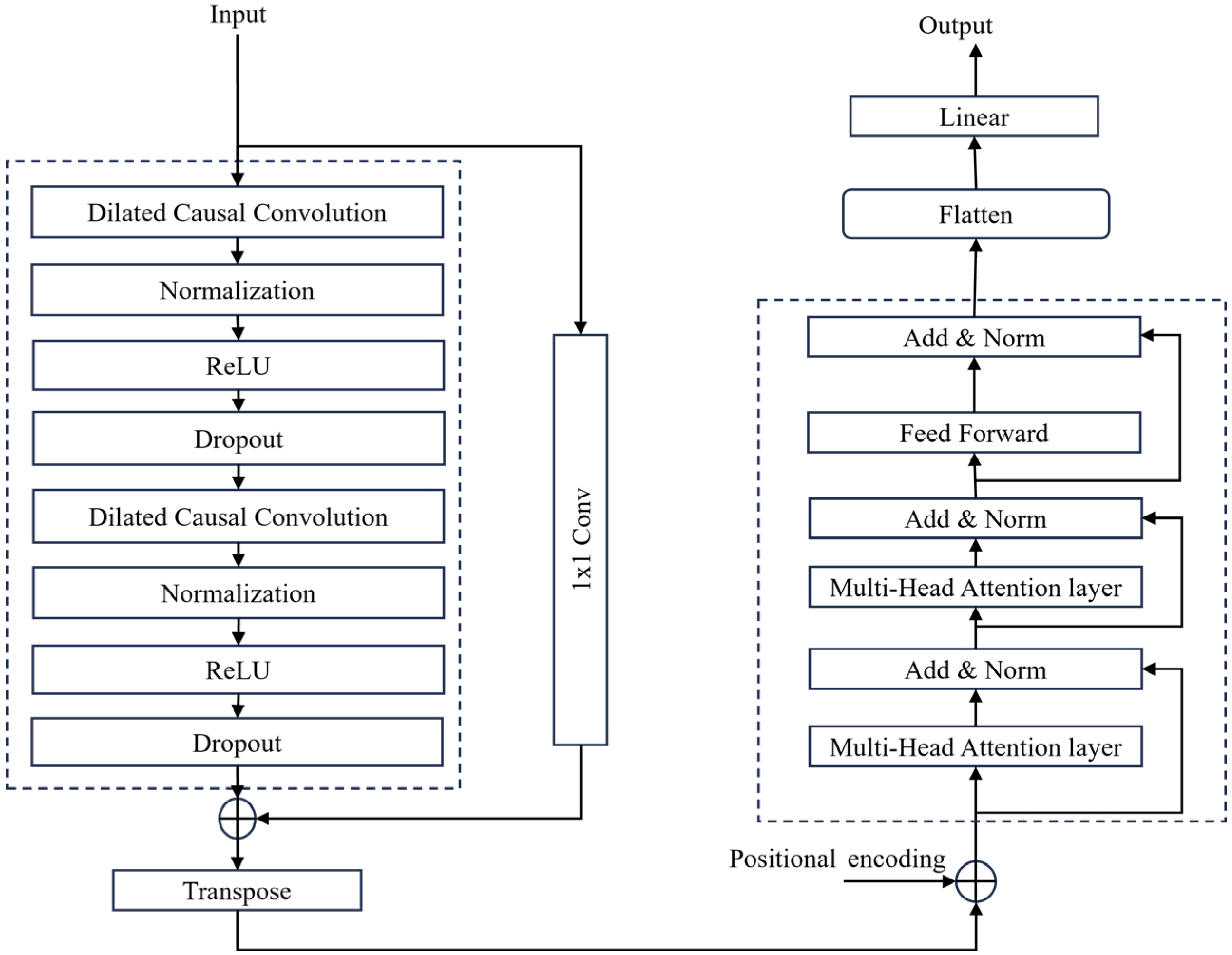
The TCN proposed by Colin Lea et al. [12] offers long-term dependency modeling capabilities compared with those of RNNs, while also combining the stable gradients and high parallel computational efficiency of convolutional neural networks (CNNs). The Transformer model, introduced by Vaswani et al. [23] in 2017, abandons traditional RNN and CNN architectures and is built on a self-attention mechanism, overcoming the limitations of inefficient training and inadequate long-range dependency modeling in RNNs. With its highly parallelizable structure, the Transformer significantly improves training speed. To address the spatiotemporal characteristics of voltage and power flow in active distribution networks, this paper integrates the advantages of TCN and Transformer models to construct a hybrid architecture: the TCN module efficiently extracts multi-level temporal features through causal dilated convolutions, ensuring gradient stability and computational efficiency; the Transformer module captures global spatiotemporal dependencies via self-attention mechanisms.

TCN module processes the input features to extract temporal patterns, which are then fed into a Transformer encoder composed of multi-head self-attention, layer normalization, and feed-forward networks. The TCN output $Y$ is computed as:

$$Y=TCN(X)={\displaystyle {\sum }_{k=1}^K}{\displaystyle {\sum }_{m=1}^M}{\alpha }_{km}\cdot X$$

(9)

where $X$ is the input feature matrix; $K$ is the number of convolutional kernels; $M$ is the dilation rate; and ${\alpha }_{km}$ represents the kernel weights.

Following the TCN module, the Transformer encoder captures global spatiotemporal dependencies via self-attention mechanisms. The Transformer’s output $W$ is given by:

$$W=Transformer(Z)=FFN(LayerNorm(Z+MultiHead(Z,Z,Z)))$$

(10)

where $Z$ is the input to the Transformer, which is the output of the TCN module; $MultiHead$ denotes the multi-head self-attention mechanism; $LayerNorm$ is layer normalization, and $FFN$ represents the feed-forward network.

The model structure is shown in Figure 5. Input features are first processed by the TCN module to extract temporal patterns and then fed into a Transformer encoder composed of multi-head self-attention, layer normalization, and feed-forward networks. This enables the synergistic integration of local feature preservation and global correlation modeling, effectively capturing the evolution patterns of voltage and power flow violation risks.

As specified by the risk assessment metrics defined in Section 3.1, the assessment of the risk of power flow and voltage violation in the distribution network relies on point forecasts and interval forecasts of the corresponding risk indicators, respectively. Accordingly, this work integrates the Lower Upper Bound Estimation (LUBE) method with the TCN-Transformer architecture by designing different loss functions, and uses the deep neural network to learn potential patterns between data, providing accurate violation risk assessments.

For point forecasting of the power flow violation risk indicator, the Mean Squared Error (MSE) is adopted as the loss function:

$$MSE={\displaystyle \frac{1}{N}}{\displaystyle \sum _{i=1}^N{(y_i-{\widehat{y}}_i)}^2}$$

(11)

where $N$ denotes the number of samples; $y_i$ and ${\widehat{y}}_i$ represent the true and the predicted values of the $i-\mathrm{th}$ sample, respectively.

On the other hand, the loss function for interval forecasting of the voltage violation risk assessment indicator is formulated by comprehensively considering the Prediction Interval Coverage Probability (PICP) and the Prediction Interval Normalized Average Width (PINAW). Since both over-voltage and under-voltage risks in the distribution network must be considered, this paper configures the maximum positive and negative voltage deviations as the two outputs of the model. The corresponding loss function, denoted as $soft\_CWC$, is defined as follows:

$$soft\_CWC={\displaystyle \frac{soft\_CW{C}_1+soft\_CW{C}_2}{2}}$$

(12)

$$Soft\_CW{C}_j=PINA{W}_j+{\lambda }_1{e}^{{\lambda }_2\max (0,PINC-PIC{P}_j)}$$

(13)

$$PINA{W}_j={\displaystyle \frac{1}{n\cdot S}}{\displaystyle \sum _{i=1}^n(U_j(X_i)-L_j(X_i))}$$

(14)

$$PIC{P}_j={\displaystyle \frac{1}{n}}{\displaystyle \sum _{i=1}^{n}soft\_k_{ij}}$$

(15)

$$soft\_k_{ij}=sigmoid(s\cdot (Y_{ij}-L_j(X_i))\times sigmoid(s\cdot (U_j(X_i)-Y_{ij})$$

(16)

where $j=1,2$ represent the maximum positive and voltage deviations, respectively; $n$ denotes the number of target sets; $U_j(X_i)$ and $L_j(X_i)$ are the predicted upper and lower bounds of the $j\text{-}\mathrm{th}$ type deviation interval for the $i\text{-}\mathrm{th}$ sample $X_i$, respectively; ${\lambda }_1$ and ${\lambda }_2$ represent penalty coefficients; S denotes the difference between the maximum and minimum values of the sample targets; $Y_{ij}$ is the true value of the $j\text{-}\mathrm{th}$ type deviation for the $i\text{-}\mathrm{th}$ sample; $s$ is the softening coefficient, and the target Prediction Interval Nominal Coverage (PINC) is a pre-set parameter.

3.3. TCN-Transformer-Based Assessment Framework for Power Flow and Voltage Violation Risks

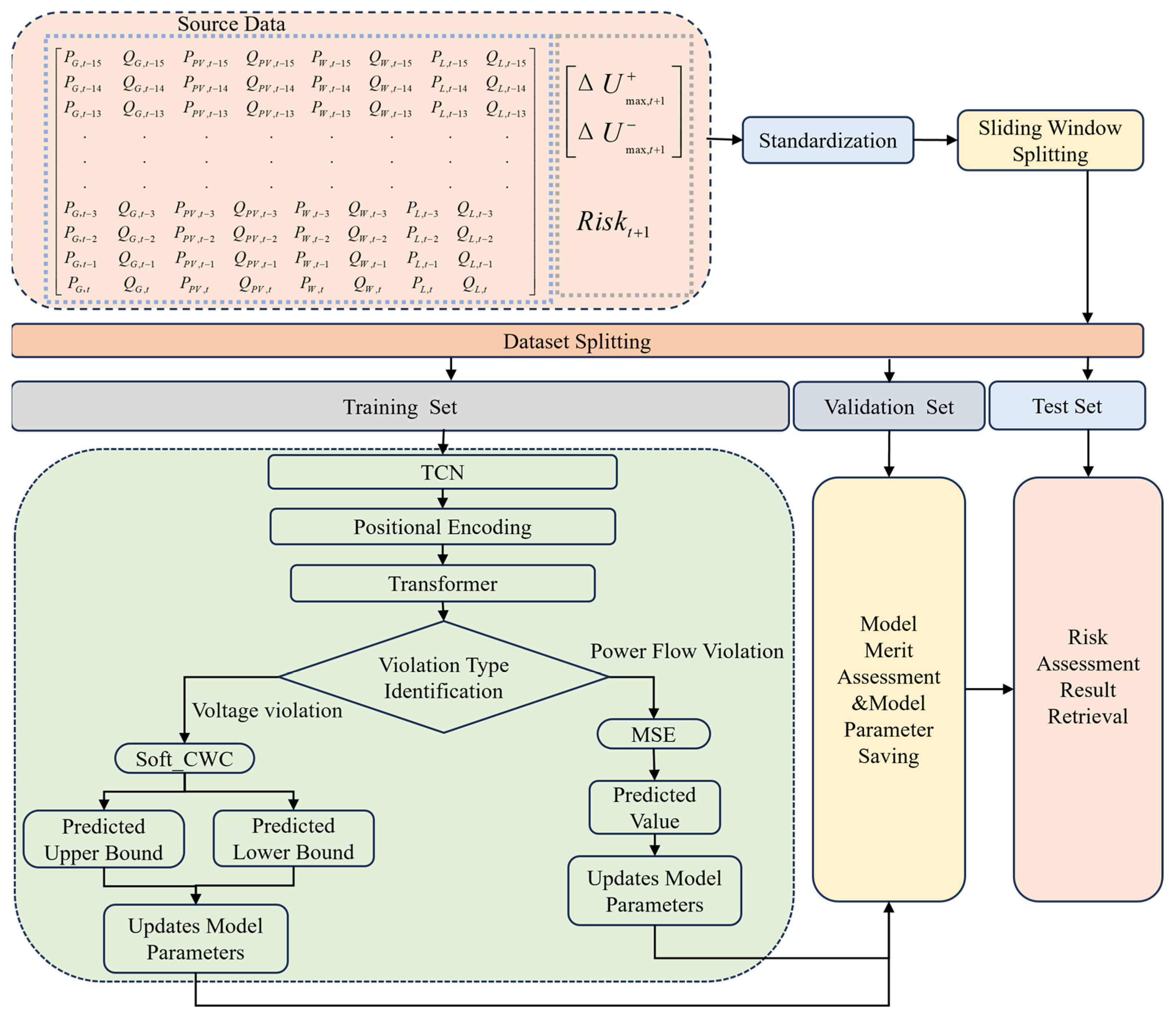
Building upon the two aforementioned loss functions, this section presents a TCN-Transformer based methodology for assessing power flow and voltage violation risks in distribution networks. The specific assessment procedure is illustrated in Figure 6.

As the spatiotemporal analysis of distribution network power flow and voltage characteristics indicates, limit violation risks are influenced by generation-load side power fluctuations. Therefore, this study selects eight input features for the risk assessment model: active power of conventional generation (P_G), reactive power of conventional generation (Q_G), active power of wind power (P_W), reactive power of wind power (Q_W), active power of photovoltaic generation (P_PV), reactive power of PV generation (Q_PV), active load power (P_L), and reactive load power (Q_L). These inputs are used to compute the maximum positive/negative voltage deviations, and power flow violation risk indicator at each time step.

To eliminate scale effects among variables in the dataset, Z-Score normalization is applied:

$$x^{\prime }={\displaystyle \frac{x-\mu }{\sigma }}$$

(17)

where $x$ represents the original input value; $\mu$ denotes the mean; and $\sigma$ represents the standard deviation.

A sliding time window approach is employed to construct the sample dataset, with a window length of $l$. Each data sample consists of an input feature matrix over $l$ consecutive time steps, along with the corresponding next-time-step values of either the maximum positive/negative voltage deviations or the power flow violation risk indicator. The sample dataset is then partitioned into training, validation, and test sets in a ratio of a:b:c.

Subsequently, the hyperparameters of the TCN-Transformer model—such as kernel_size, tcn_channels, d_model, nhead, and dropout—are initialized. The appropriate loss function is selected based on the specific assessment task. The model is trained using the training set, and at the end of each epoch, the validation set is used to evaluate performance and determine whether the current optimal model has been obtained via the Adam optimization algorithm.

Finally, the test set is fed into the optimal model to obtain either forecasting values of the power flow violation risk indicators or prediction intervals for the maximum positive/negative voltage deviations. For the predicted values of the power flow risk indicators, a higher value indicates greater risk of power flow violation, and vice versa. Additionally, the performance of the point prediction model for power flow risk is evaluated using the metrics Mean Absolute Error ($MAE$), Root Mean Square Error ($RMSE$), and Coefficient of Determination ($R^2$), as defined below:

$$MAE={\displaystyle \frac{1}{N}}{\displaystyle \sum _{i=1}^N\left|y_i-{\widehat{y}}_i\right|}$$

(18)

$$RMSE=\sqrt{{\displaystyle \frac{1}{N}}{\displaystyle \sum _{i=1}^N{(y_i-{\widehat{y}}_i)}^2}}$$

(19)

$$R^2=1-{\displaystyle \frac{{\displaystyle \sum _{i=1}^N{(y_i-{\widehat{y}}_i)}^2}}{{\displaystyle \sum _{i=1}^N{(y_i-{\overline{y}}_i)}^2}}}$$

(20)

For the prediction intervals of the maximum positive and negative voltage deviations, the indicators PICP and PINAW are selected as evaluation metrics to assess the performance of the interval forecasting model. Furthermore, by comparing the predicted voltage fluctuation intervals with the safe operational thresholds, the following conclusions can be drawn. In the case of the maximum positive voltage deviation, if both the upper and lower prediction bounds exceed the safe threshold, there is a very high risk of overvoltage; if the upper bound exceeds the threshold while the lower bound remains within it, a moderate overvoltage risk is indicated; and if neither bound surpasses the threshold, the overvoltage risk is considered very low. Similar conclusions can be drawn regarding the maximum negative voltage deviation.

4. Case Study

To validate the effectiveness of the proposed risk assessment method for limit violations, case studies on both voltage and power flow violation risks in a distribution network are conducted. All experiments in this study are implemented based on the PyTorch (version 1.10.2+cu102) framework. The experimental environment consists of an Ubuntu18.04.6LTS operating system, a Montage Jintide^® C5218R CPU (Montage Technology Co., Ltd., Shanghai, China), and Python 3.6.9. Additionally, due to the extensive matrix operations involved, the NumPy (1.19.5) and Pandas (1.1.5) libraries are used in Python, while the Joblib (1.1.0) library is employed to save and load scalers and models, and Plotly (5.4.0) is used for visualization.

4.1. Dataset Generation

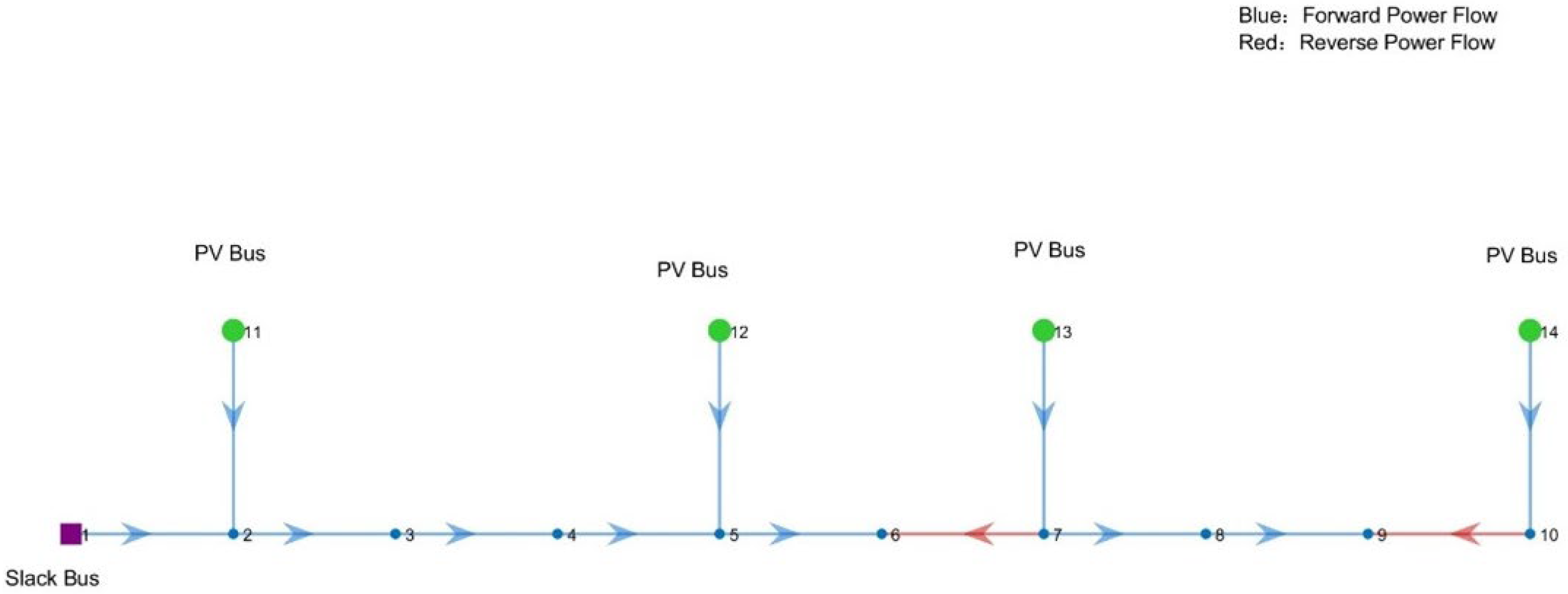
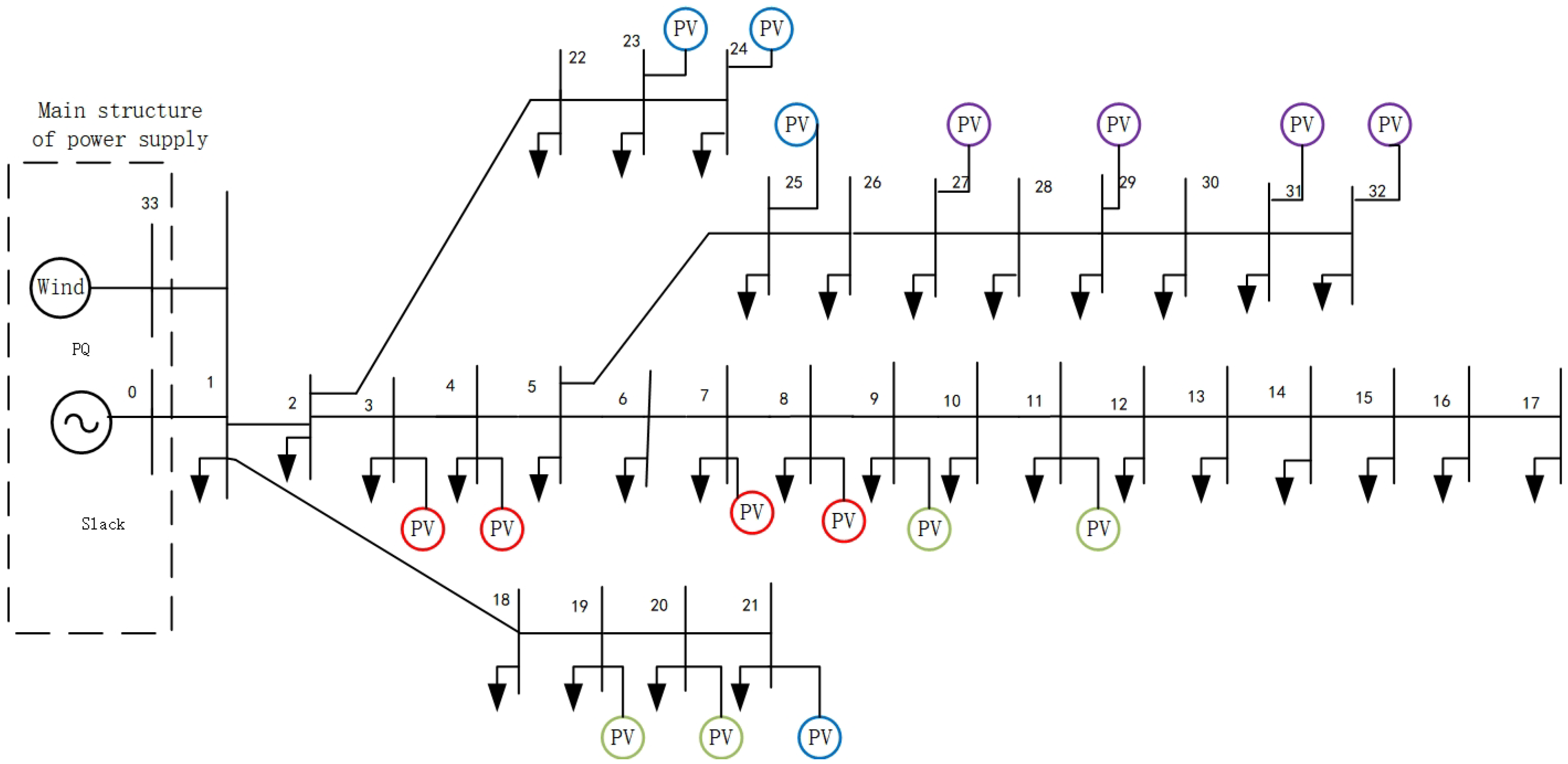
Based on a modified IEEE 33-node distribution network model, an active distribution network simulation model is developed in MATLAB (2023b), as illustrated in Figure 7. To incorporate temporal characteristics, multiple operational scenarios are constructed by combining various conditions, including no photovoltaic (PV) generation, low PV generation, high PV generation, light load, and heavy load. Typical daily load profiles and PV output curves for different seasons are considered. Annual time-series data of conventional generation, centralized wind power, distributed PV output, and load power are used as inputs, with a time step of 15 min. The corresponding outputs include the future maximum positive/negative voltage deviations, and the comprehensive power flow violation risk indicator. Meanwhile, considering the spatial characteristics, the distributed energy resources are connected to 4 different feeders to simulate various integration locations, such as the beginning, the end, and dispersed points along the feeders.

The parameters of the simulation model are summarized in

Table 1. Key Parameter Configurations of the Simulation Model.

Parameter	Value
Rated Voltage	10 kV
Distributed PV Capacity	1 MW
Wind Power Capacity	16 MW
Total Load	2 MW~6 MW
Main Feeder Ampacity	400 A
Branch Line Ampacity	200 A

. Based on the simulated data, a dataset comprising 35,040 samples—each consisting of an input feature matrix and an output label matrix—is constructed. This dataset comprehensively captures the operational characteristics of active distribution networks, providing substantial data support for training and validating the proposed risk assessment model for distribution network limit violations.

4.2. Case Study on Power Flow Violation Risk Assessment

To validate the effectiveness and superiority of the proposed model for power flow violation risk assessment, comparative experiments are conducted using LSTM, Transformer, and TCN-Transformer models with the loss function defined in Equation (11). The dataset generated in Section 4.1 is processed using a sliding time window with a length of 16 to construct the sample dataset, which is then divided into training, validation, and test sets in a ratio of 6:2:2. This resulted in 21,015 training samples, 7006 validation samples, and 7006 test samples. The input consists of 128 feature values formed by the 8 input features from the previous 16 time steps, and the output is the power flow violation risk indicator for the next time step.

The parameter settings of the proposed model are summarized in

Table 2. Parameter configuration of the TCN-Transformer model.

Parameter	Value
num_channels	[32, 64]
kernel_size	3
dropout	0.2
d_model	64
nhead	4
num_layers	2
dim_feedforward	256

. For fair comparison, the corresponding hyperparameters in the Transformer and TCN-Transformer models are kept consistent with those of the proposed model. The LSTM model is configured with hidden_size = 64 and num_layers = 2, while all other parameters remained the same as in the proposed model. These models are trained for 200 epochs with a learning rate of 0.001.

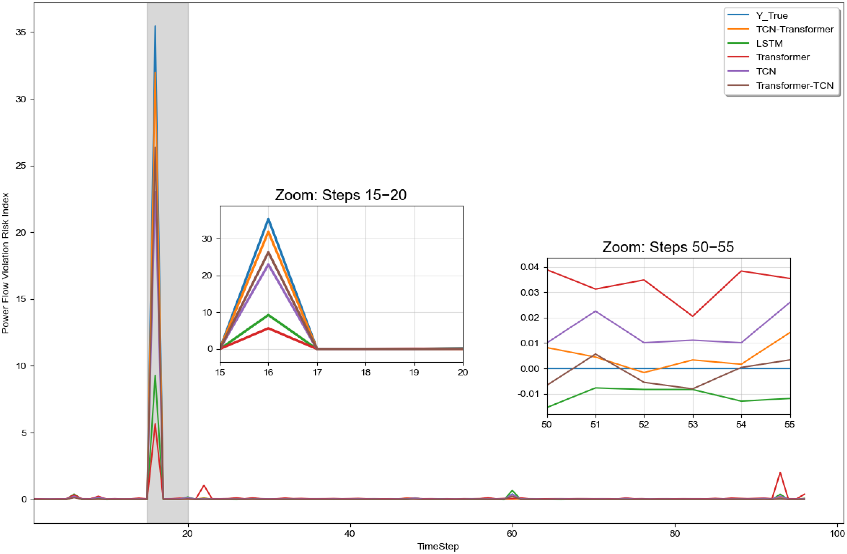
On a randomly selected day in the test set, Figure 8 shows the prediction curves of power flow violation risk indicators for different models. During normal operation, the curves remain around zero, indicating minimal risk. Between sampling points 15–20, a sharp increase occurs in all curves, reflecting serious violations. As shown in the enlarged view, the proposed TCN-Transformer model demonstrates superior alignment with the ground truth compared to other three models. Furthermore, between sampling points 50–55, the proposed model exhibits predictions closer to zero and smoother behavior under normal conditions.

To comprehensively evaluate the performance of each model,

Table 3. The comparison of the performance indicators for different power flow violation risk assessment models on the entire test set.

Model	RMSE	MAE	R2
TCN-Transformer	0.651	0.059	0.761
LSTM	0.881	0.066	0.562
Transformer	1.203	0.139	0.182
Transformer-TCN	0.804	0.098	0.635
TCN	0.786	0.062	0.651

presents a comparison of the prediction performance metrics of all models on the entire test set. The results demonstrate that the TCN-Transformer model achieves the best performance in terms of both prediction error and model goodness-of-fit. Specifically, it attains values of 0.651 for RMSE, 0.059 for MAE, and 0.761 for R² across the three key metrics. These results confirm the superiority of the proposed TCN-Transformer model in assessing power flow violation risks.

In summary, the proposed model can achieve best prediction performance. The power flow violation risk indicator predicted by the TCN-Transformer model quantitatively reflects the security level. A value of 0 indicates no risk of power flow violation in the distribution network, while a larger value corresponds to a higher risk of power flow violation.

4.3. Case Study on Voltage Violation Risk Assessment

Based on the aforementioned models, this subsection conducts comparative experiments for voltage violation risk assessment with the loss function specified in Equation (12). The parameter configurations of all models remain consistent with those in Section 4.2. The input continues to consist of 128 feature values, while the outputs are the maximum positive voltage deviation $\Delta U_{\max }^{+}$ and the maximum negative voltage deviation $\Delta U_{\max }^{-}$ at the next time step. The learning rate is set to be 0.001 and the training duration is 100 epochs. An early stopping mechanism is incorporated with a patience value of 20.

The loss function achieves a balanced optimization between coverage and interval width through four core parameters. Among them, the softening coefficient $s$ of 5, PINC of the target prediction interval is 0.9, penalty coefficients λ₁ = 50 and λ₂ = 0.2. As a result, the loss function not only strictly constrains the lower bound of the prediction interval coverage but also minimizes the interval width, accomplishing the prediction objective of high coverage and narrow width.

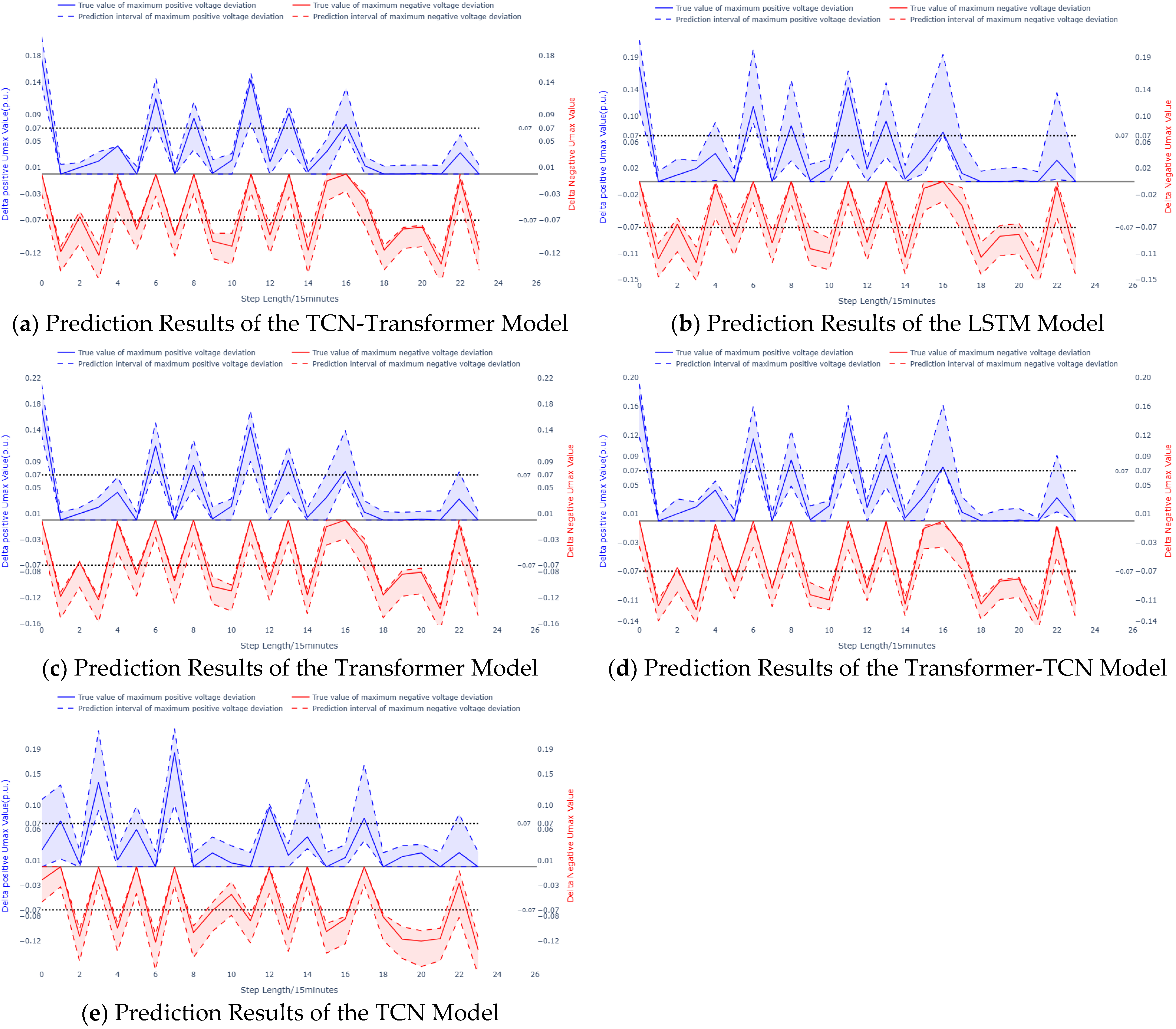
Figure 9 present the prediction results of each model for 24 consecutive sampling points. In the figures, the solid blue/red lines represent the true values of the maximum positive/negative voltage deviations, while the blue/red dashed lines indicate the upper and lower prediction bounds for the maximum positive/negative voltage deviations. The safe threshold for voltage deviation in the 10 kV distribution network is set at ±0.07 pu, denoted by gray dashed lines.

As observed in Figure 9d, the Transformer-TCN model fails to cover the true values at sampling point 16, whereas the prediction bounds of the proposed model fully encapsulate the true values in Figure 9a. From the figures, there exists an extremely high risk of undervoltage violation at sampling point 20. However, the upper prediction bound for the maximum voltage negative deviation of the LSTM model remains within the safe voltage range in Figure 9b, thereby reducing its accuracy in assessing the undervoltage risk. Additionally, the proposed model exhibits narrower prediction intervals overall compared to the Transformer model in Figure 9c and the TCN model in Figure 9e. Therefore, as shown in the figures, the proposed TCN-Transformer model has certain advantages in interval coverage and interval width.

By analyzing the output prediction intervals at each sampling point, i.e., determining whether the upper and lower bounds exceed the safe voltage deviation threshold, the risk of overvoltage or undervoltage violations can be effectively assessed. As shown in Figure 9a, an extremely high risk of undervoltage violation is observed at sampling point 10, accompanied by a moderate risk of overvoltage violation. At sampling point 13, a moderate overvoltage violation risk is identified, while the risk of undervoltage violation remains very low. At sampling point 22, both overvoltage and undervoltage violation risks are assessed to be very low.

In order to comprehensively evaluate the interval prediction performance,

Table 4. The comparison of the performance indicators for different voltage violation risk assessment models on the entire test set.

Model	PICP1	PINAW1	PICP2	PINAW2
TCN-Transformer	0.9136	0.0531	0.9005	0.0693
LSTM	0.9246	0.0643	0.9152	0.0734
Transformer	0.9209	0.0613	0.9154	0.0728
Transformer-TCN	0.9257	0.0654	0.9325	0.0788
TCN	0.9289	0.0649	0.9190	0.0735

presents a comparison of the performance indicators of all models on the entire test set. Figure 10 visualizes the comparison results of the above performance indicators. The results indicate that the proposed model and the comparative models have achieved the specified PINC. Meanwhile, the proposed model yields PINAW₁ = 0.053 and PINAW₂ = 0.069, which represent the narrowest interval widths among all outputs. This indicates that the proposed interval prediction model provides more precise prediction intervals while meeting the accuracy requirements for voltage violation risk assessment.

5. Conclusions

To address the challenge of risk assessment for limit violations in active distribution networks, this study has undertaken a two-pronged approach. On one hand, a comprehensive evaluation index system has been proposed, incorporating the maximum positive/negative voltage deviations, and a composite power flow violation risk indicator, based on an in-depth analysis of the spatiotemporal correlations inherent in power flow distribution and voltage characteristics. On the other hand, a TCN-Transformer based risk assessment model has been developed to effectively capture the influence of various features on distribution network violation risks. Furthermore, by modifying the network loss function, the model achieves accurate point predictions for power flow violation indicator and interval forecasts for extreme voltage deviations.

Case study results demonstrate the significant advantages of the proposed method in assessment accuracy. It retains the interpretability of physical mechanisms characteristic of traditional methods, thereby aligning with the physical principles governing distribution network operation. Simultaneously, it fully leverages the feature extraction and self-learning capabilities of the TCN-Transformer deep neural architecture to effectively capture spatiotemporally correlated characteristics and improve assessment precision. This work provides a new pathway for the practical application of artificial intelligence technology in the field of distribution network violation risk assessment.

However, enhancing the model’s generalization capability across distribution systems with varying topological structures and developing adaptive optimization strategies remain important challenges. Furthermore, as the frequency support capability of the main grid declines in the future, frequency violation risk in distribution networks will become an important research direction. Future research will focus on improving the robustness of the model and exploring frequency stability issues so as to offer more accurate technical support for risk early-warning and control decision-making in active distribution networks.