Abstract
Aiming at the problem that the well depth parameters in existing intelligent drilling technology can not be obtained underground, a multi-branch parallel neural network is proposed to solve the problem of downhole well depth tracking, and its effectiveness is verified by a field example. After analyzing and correcting the quality of the logging data collected on site by using DBSCAN (a density clustering algorithm), five parameters of WOB, rotating speed, displacement, pump pressure, and torque are selected to predict and calculate the downhole mechanical ROP. Adjust the structure of a traditional artificial BP neural network and design a multi-branch parallel neural network, change the basic architecture of the original hierarchical operation, make full use of the operation efficiency of a computer to realize parallel operation, and adopt the method of point-to-point depth comparison when evaluating the well depth tracking effect. The results indicate that the MAE and mechanical drilling rate evaluation values obtained were 1.18 and 0.873, respectively. The multi-branch parallel neural network achieved a 66.55% improvement in MAE compared to the original BP neural network, while the R2 evaluation method showed a 61.82% increase. The average point-by-point comparison error in the example calculation was 0.012 m, with a maximum error of 0.268 m. This result can serve as a fundamental basis for judging changes in well depth during the drilling process.
1. Introduction
To improve encounter rates, drilling efficiency, and wellbore quality in the oil and gas industry, intelligent drilling technology is an inevitable development [1]. This technology integrates big data, digitalization, and artificial intelligence systems. It uses precise downhole sensors to control the drill bit autonomously and manage integrated operations comprehensively. Intelligent drilling requires the sequential completion of three objectives: downhole depth tracking, formation identification, and automatic wellbore trajectory optimization. Depth tracking is the foundational element of the entire system. Currently, the well’s deviation angle and azimuth can be obtained directly from downhole instruments during intelligent drilling. In related research, Noureldin, A et al. [2] noted that horizontal drilling commonly employs triaxial magnetometers and accelerometers within measurement-while-drilling (MWD) systems to measure the wellbore. The former provides real-time azimuth, and the latter outputs the tool face angle (roll angle) and vertical deviation angle (pitch angle) after processing. However, soft rock is prone to collapse, wellbore walls deform easily, and drill string vibration is pronounced. Traditional magnetometer measurements rely on expensive non-magnetic drill collars and suffer reduced accuracy due to the influence of steel components surrounding drilling equipment and geomagnetic field shifts. In contrast, the fiber optic gyroscope (FOG) mentioned in this study exhibits excellent interference resistance in harsh downhole environments and offers a new approach to measuring wellbore trajectories in soft rock drilling. However, well depth parameters still rely on traditional counting-drill-pipes methods, combined with uploaded wellbore inclination and azimuth data to calculate the wellbore trajectory. This trajectory is then adjusted and controlled based on the designed path and actual geological conditions. To achieve truly intelligent drilling, real-time acquisition of well depth parameters downhole is essential to support autonomous decision-making and control of drilling tools. Therefore, the implementation of downhole well depth tracking is of critical importance [3].
To address this challenge, researchers worldwide have proposed various approaches. For example, Yan et al. [4] employed a random forest method to predict azimuth, deviation angle, and bit angle. While this data-driven approach avoids complex modeling, it struggles to capture temporal correlations and dynamic features in sequential data. This results in poor adaptability to time-series data, challenging parameter tuning, and suboptimal prediction performance. To improve prediction accuracy, Wang et al. [5] and Shan et al. [6] used LSTM and CNN-LSTM hybrid models, respectively, to predict logging data for undrilled sections using neighboring well logs and achieved favorable results. However, predictions may become inaccurate when the distance between neighboring wells is too great or when well-to-well correlations are weak. This method is particularly challenging when there is insufficient neighboring well data at the target prediction depth.
Backpropagation (BP) neural networks have garnered significant attention for their outstanding self-learning capabilities, adaptability, robustness, and generalization performance, finding successful applications across multiple engineering domains. Research indicates their potential in drilling parameter prediction. For instance, Li Qi et al. [7] employed a particle swarm optimization (PSO) algorithm to optimize a BP network for predicting the mechanical rate of penetration (ROP), effectively enhancing prediction accuracy. Lawal A I [8] combined the antlion optimization algorithm with artificial neural networks for ROP prediction; Su K [9] proposed using an improved chaotic whale optimization algorithm (ICWOA) to optimize BP neural network weights, further enhancing ROP prediction accuracy; Avcı E [10] applied an ANN to predict the rheological properties of water-based drilling fluids. However, widespread application has also highlighted inherent limitations of BP neural networks: their susceptibility to local optima, the lack of theoretical guidance in network architecture design (often relying on empirical trial-and-error), and issues such as gradient vanishing, training instability, and slow convergence.
Addressing these limitations, this paper proposes integrating drilling rate-related data with a multi-branch parallel artificial neural network to develop a downhole well depth tracking calculation method. This approach aims to provide new insights for theoretical research and technological implementation in this field.
2. Well Logging Data Preprocessing
The prediction effect of underground well depth tracking is related to the quality of logging data used in training, and the factors affecting the quality of logging data are usually related to manual recording errors and improper machine operation. In order to ensure the accuracy of underground well depth tracking, the logging data should be preprocessed before calculation, mainly to eliminate the actual data containing a small amount of errors caused by labor or machines. The density clustering algorithm (DBSCAN) is a class of unsupervised learning algorithms [11], commonly used in classification labeling data; this paper uses DBSCAN’s classification labeling characteristics to invert DBSCAN’s outlier removal function for the quality analysis and correction of logging data.
2.1. Standardized Processing of Data
The actual logging data has multiple columns of characteristics, such as drilling pressure, speed, displacement, pumping pressure, torque, etc. [12], and the numerical relationship between the characteristics of each column may differ by several times or dozens of times, which will cause problems such as dimensional explosion and excessive computing resource occupation, so it is necessary to standardize the logging data before removing the outliers, compress the data to −1 to 1, and prevent excessive deviation between the data from leading to unsatisfactory training results and large errors [13]. The standardized formula is as follows:
In the formula, is the normalized data, the is the original data, is the mean of the data, and the σ is the variance of the data.
After the data standardization operation, the density clustering algorithm (DBSCAN) was used in the outlier exclusion part of the downhole depth tracking calculation model, and the maximum density-connected sample collection was derived from the density reachability relationship [14].
2.2. Outlier Culling
The actual data obtained in the field often contains a small amount of error caused by labor or machines, and in order to ensure the accuracy of the model’s prediction of mechanical drilling speed, it is necessary to eliminate the outlier value of the data to eliminate the error.
Figure 1 is the algorithm core diagram of the DBSCAN in the above process, Figure 1 can be understood as the point close to the boundary in the figure is the boundary point, because within the radius Eps, the number of points in its domain do not exceed MinPts, assuming that the MinPts set is 5. The middle point is the core point because the points in its neighborhood are more than MinPts points; through this clustering method, some of the outliers caused by on-site recording errors or equipment errors can be eliminated, and data that are more effective for the algorithm can be obtained.
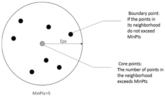
Figure 1.
DBSCAN denoising principle.
In the process of intelligent drilling data acquisition, there is usually no “dimensional disaster” of logging data caused by a too high data dimension, so the selection of the measurement function of distance directly affects the effect of outlier elimination [15], DBSCAN clustering quality depends on the selection of the distance formula, and the best distance measurement function in the actual application process is Euclidian distance:
In the formula, and are points in n-dimensional space, and n represents the amount of dimension.
When selecting by Euclidean distance and forming a density reachable cluster, it is necessary to further determine the density reachable cluster, because there may be points with reasonable data logic that are not in line with the logging data logic, so it is necessary to further determine the distance of the density reachable cluster, and the determination method adopts the average distance calculation formula [16]:
In the formula, represents the k points closest to the point .
It can be seen from Equation (3) that the smaller the average distance, the greater the density around the data point, and the density reachable cluster can be formed through the Euclidean distance, and then the average distance is used to screen the logging data. DBSCAN employs a grid search for hyperparameter tuning, a method also known as grid search. Its core logic involves processing hyperparameters in a grid format: first defining an initial set of values for each hyperparameter, then systematically searching through all possible combinations within the grid. During the iterative search process, trial-and-error approaches are used to screen parameter combinations. The configuration that achieves a balance between overfitting and underfitting represents the model’s optimal fit. By adjusting different types of hyperparameters—such as the learning rate and weights—the model’s learning process can be effectively controlled. This enables the discovery of inherent hidden patterns within the data across corresponding datasets for similar machine learning models. Following comprehensive grid parameter tuning validation, the optimal hyperparameters for the DBSCAN were finalized as eps = 0.8 and min_samples = 100. Which can realize the correction of outlier values of the logging data and eliminate the influence of manual error or machine error on the subsequent downhole depth tracking [10].
3. Calculation Model for Downhole Depth Tracking
For the calculation of downhole depth tracking, this paper proposes a calculation model. The model mainly includes the multi-branch parallel neural network and well depth tracking evaluation method obtained after the improvement of the structure of the traditional artificial BP neural network. The downhole depth tracking calculation model can select different drilling characteristic parameters as input quantities according to the actual logging data of different sites, and can flexibly realize downhole depth tracking.
3.1. Multi-Branch Parallel Neural Networks
Traditional artificial BP neural networks, also called backpropagation neural networks, improve their computational regression capabilities because they contain many hidden layers. It is precisely because of the backpropagation algorithm that the training of the neural network converges quickly, and the learned neural network has also reached a practical level. The training process of a BP neural network consists of the forward transmission of data and the reverse propagation of gradients. Forward propagation is the process that passes the weighted sum of data through one or more hidden layers and then passes it to the output layer; if the output does not match the true value, the gradient of the error is passed in reverse layer by layer, so that each training parameter can be updated, and the loss function will be minimized, so as to find the optimal solution or suboptimal solution of the neural network [17].
However, the BP neural network model also has many shortcomings, such as the fact that it is easy for the BP neural network model to fall into the local optimal solution instead of the global optimal solution; the structure of the model can only be optimized by experience without exact theoretical support; BP neural networks require a large number of parameters, such as the network topology, the initial values of weights and thresholds; the learning process of BP neural networks cannot be visualized [18]. Based on the above problems, this paper starts from the traditional structure of a BP neural network and establishes a multi-branch parallel neural network model to solve the regression problem and optimize the traditional BP neural network model.
The main operation process of the traditional BP neural network model is to input data through the input neural unit of the input layer, then linearly superimpose the neurons layer by layer through the hidden layer, and continue to pass parameters to the next layer in a weighted sum manner, until it is transmitted to the output layer for the budget of the result, and the error is passed backward layer by layer through the comparison of labels in the dataset, the cycle is repeated, and the optimal solution under the existing conditions is solved again and again by iteration, but usually the suboptimal solution is obtained, because the optimal solution cannot be obtained [19]. The operation steps of the improved multi-branch parallel neural network are different from the above traditional BP neural network operation process; the operation of the multi-branch parallel neural network is not a hierarchical operation, but from the input neural unit to the separate four branches, the data through the input layer is directly synchronized into the four hidden layer branches for synchronous calculation, and the calculated data is budgeted in two branches for the maximum, and then passed to the next neuron, and finally only two parts of neurons receive the data, the obtained data is passed to the output layer after the minimum operation, and then compared with the real value and then passed in reverse, and finally the suboptimal solution is obtained after gradual iteration (Figure 2).
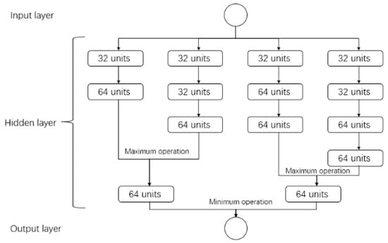
Figure 2.
Multi-branch parallel neural network model.
In the multi-branch parallel neural network model, the input information adopts the five parameters of drilling, pressure, speed, displacement, pump pressure, and torque, in the logging data, and the drilling pressure, speed, displacement, pump pressure, and torque are expressed by , and the input layer is expressed in vector form: . The hidden layer has a total of four branches, and the output information of each branch is expressed in vector form: . One neuron in the output layer is used to output the predicted mechanical drilling speed, and the vector form of the mechanical drilling speed is represented by . The true mechanical drilling speed value is expressed as the desired output vector, and the vector form of the desired output is represented by . The weight between the input layer and the hidden layer is expressed by the matrix V, , where the vector represents the connection weight corresponding to the j neuron of the hidden layer. The weight between the hidden layer and the output layer is expressed by the matrix W, , where the vector represents the connection weight corresponding to the k neuron of the output layer.
For the hidden layer activation function, in order to avoid the problem of gradient disappearance [20], the SELU function is used to activate the hidden layer (Figure 3), and the formula of the SELU function is as follows:

Figure 3.
SELU function image.
In SELU’s formula, a represents the phased result obtained after entering the five parameters of drilling pressure, speed, displacement, pump pressure, and torque into each layer of the multi-branch parallel neural network. It can be seen from the formula and image of SELU that the derivative of the positive semi-axis of the activation function is always greater than 1, which will make the data variance increase when it is too small, while the negative half axis is not directly converted to 0, but uses a smaller slope function to avoid the problem of gradient disappearance, and also effectively plays to the advantage of unilateral suppression [21].
The hidden layer formula is listed as follows:
The formula for the result of the mechanical drilling speed output by the output layer is as follows:
After calculating the predicted value of the mechanical drilling speed, the downhole depth tracking model is obtained by multiplying the predicted value vector of mechanical drilling speed by the data flow interval t of logging data, and the well depth L calculation formula is as follows:
In the traditional training process, SGD (stochastic gradient descent) is mostly used as an optimizer to optimize the gradient, but the disadvantage of traditional SGD is that the learning rate is single and not flexible enough, resulting in an easy inability to quickly find the lowest point of the optimized function and it may fall into the local optimal solution, also known as the saddle point. In order to solve this problem, the Adam optimization algorithm is used to replace SGD in the training process; the advantage of this is that it can design independent adaptive learning rates for different parameters by calculating the first-order moment estimation and second-order moment estimation of the gradient according to the change in gradient, and it has high computational efficiency and low memory requirements, so it is not easy for Adam to fall into a local optimal solution and the update speed is fast [22]; the Adam update formula is as follows:
In the formula, t is the initial step; is the gradient of the stochastic objective function; is a random objective function with parameter ; is a partial first-order moment estimate, and the is equal to 0; is a partial second-order moment estimate, and the is equal to 0; is the learning rate; and are the exponential attenuation rates of moment estimation; is a positive performance number to prevent the denominator from being 0.
Through the above structural optimization, the multi-branch parallel neural network model has a very good effect on the improvement of the traditional model, and can learn better features without too many neural units, which effectively reduces the risk of overfitting.
3.2. Evaluation Methodology
For the accuracy judgment of well depth tracking, this paper uses traditional judgment methods, such as and MAE algorithms, and depth comparison methods point by point according to the time interval of data flow, and the formulas of the and MAE algorithms are as follows:
In the formula, represents the sum of squares of the residuals, represents the sum of squares of total dispersion, represents the sum of regression squares, m represents the amount of data, represents the true value, and represents the predicted value.
The mathematical meaning of R2 is goodness-of-fit; the greater the goodness-of-fit, the higher the degree of interpretation of the dependent variable by the independent variable, the change caused by the independent variable is a high percentage of the total change, and the closer the value is to 1, the higher the degree of explanation. The greater the goodness-of-fit in depth tracking, the greater the influence of the current drilling parameters on the well depth, and the more it can explain the relationship between the drilling parameters and the well depth. MAE represents the mean of the absolute value of the deviation of all individual observations from the arithmetic mean, with smaller MAEs indicating better models [23].
In order to further verify the accuracy of well depth tracking, this paper adopts the method of depth comparison point by point according to the time interval of the data flow, obtains the predicted cumulative drilling data obtained from the interval according to the two sets of data in the test set, and compares the predicted data with the true cumulative drill data.
4. Instance Calculation
In current drilling practice, at least in China, there has not been a downhole depth tracking test, and no data has been directly obtained downhole to verify the method [24], and this paper only collects data at the surface. For this purpose, data on a total of 10 wells in a block was obtained at the field site, and the mud and drilling tool combination used in this block were the same. Take nine wells as a training set, one well as a test set, a total of 13,830 sets of data, considering that the obtained data is inaccurate, unreasonable, etc., so the data is preprocessed for the above logging data; mainly the data outlier value is removed and corrected, and finally the cleaned data has a total of 7719 sets. The drilling pressure, speed, displacement, pumping pressure, torque in the obtained logging data in the five parameters are input vectors , brought into Equations (5)–(8) to predict the downhole mechanical drilling speed [25].
All the data are randomly scrambled and split into a training set and a test set, of which the proportion of the test set is 10% [26], the processed raw data is input into the multi-branch parallel neural network learning model, and the gradient is continuously calculated according to the principle of minimizing MSE to minimize the loss function and constantly update the neural network parameters. The specific training process is shown in Figure 4:
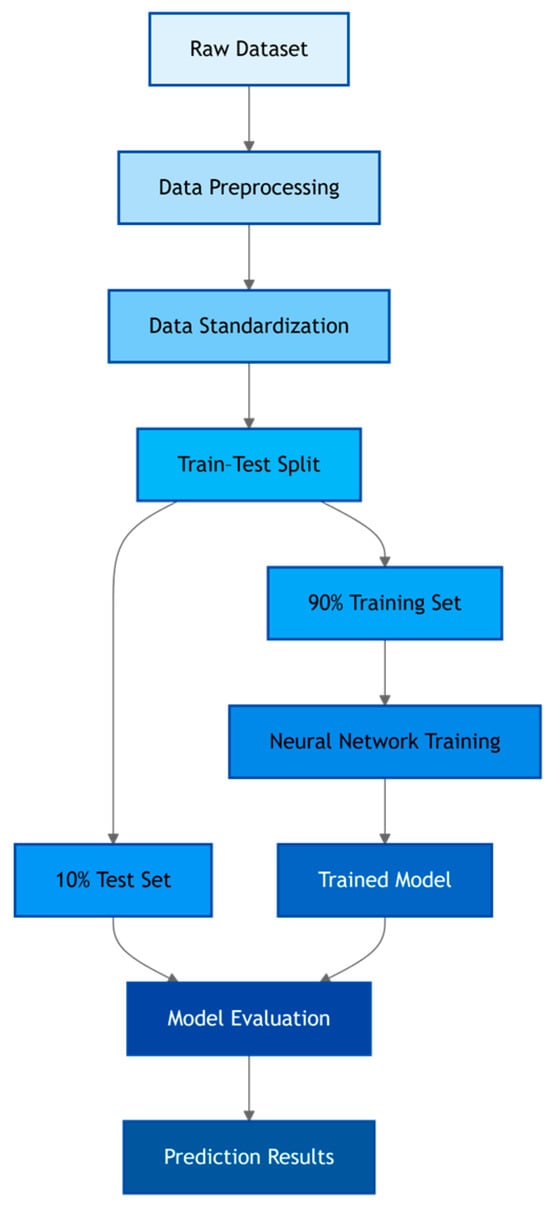
Figure 4.
Training flow chart of neural network model.
The processed data is entered into the network model, and the resulting MAE and loss images are shown in Figure 5.
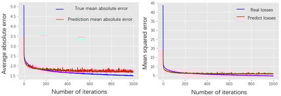
Figure 5.
MAE error curve and loss curve.
The results indicate that at 1000 iterations, the network exhibits no significant overfitting and shows no discernible trend of error reduction. Therefore, setting the training cycle to 1000 iterations is considered reasonable. On the test set, the MAE of the actual data was 1.18, R2 was 0.873, and the training time was 129 s. To demonstrate the advantages of the multi-branch parallel neural network, a comparative experiment with the original BP neural network was designed. First, dataset consistency was ensured: the original BP neural network used the same data, with identical dataset partitioning methods and preprocessing approaches to avoid data bias affecting the comparison results. Parameter tuning was also standardized, with the optimal parameter combination selected for testing. This ensured that the original BP network competed under “optimal conditions,” preventing baseline performance underestimation due to suboptimal parameter settings. As shown in Figure 6, the multi-branch parallel neural network achieved a 66.55% improvement in MAE and a 61.82% increase in R2 evaluation compared to the original BP network. This sufficiently demonstrates that the multi-branch parallel neural network exhibits excellent learning capabilities, effectively capturing overall trends within the data.
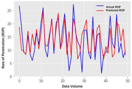
Figure 6.
Multi-branch parallel neural network mechanical drilling speed chart.
As shown in Figure 7, the test set depth is between 2143 m and 2328 m, the results are analyzed segment by segment, the average error is 0.012 m, and the maximum error is 0.268 m. According to national standards [27], the measurement error requirement for borehole depth parameters is no more than 0.20 m per single borehole. Therefore, the errors in this study meet the requirements of actual engineering projects.
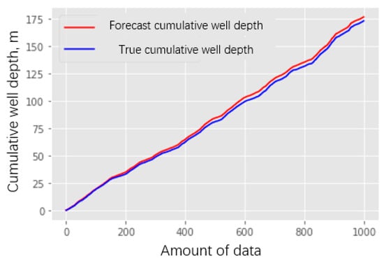
Figure 7.
Cumulative well depth curve.
In order to facilitate observation, the error between the true value and the predicted value is taken every 10 points in 1000 data points, where the 0 scale mark is the 0 error line, that is, the real value is equal to the predicted value; the closer the error point is to the 0 scale mark, the smaller the error between the true value and the predicted value, and the farther away the error point is from the 0 scale line, the larger the error between the true value and the predicted value. The error between the true and predicted values of this segment is shown in Figure 8, which shows that the multi-branch parallel neural network modeling method is reasonable and can meet the engineering requirements of downhole depth tracking [7].
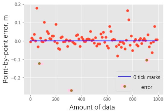
Figure 8.
Point-by-point error analysis diagram.
5. Conclusions
- (1)
- For the first time, the calculation method and evaluation method of underground well depth tracking were proposed, the traditional neural network was innovatively improved in structure, and a multi-branch parallel neural network was designed and used to realize underground well depth tracking. Compared to the original BP neural network, the MAE improved by 66.55%, and the R2 evaluation method improved by 61.82%. An evaluation method for point-by-point analysis and comparison of well depth was established.
- (2)
- In pass instance validation, the multi-branch parallel neural network takes 129 s after 1000 iterations of training, the average error of the point-by-point comparison calculated by the example is 0.012 m, and the maximum error is 0.268 m, which can meet the engineering requirements of underground depth tracking.
- (3)
- In this paper, the five parameters of drilling, pressure, speed, displacement, pump pressure, and torque, are selected to predict and calculate the downhole depth tracking. If the data is collected downhole, more and more accurate parameters such as drill bit pressure drop and geological parameters can be collected, and the effect of prediction calculation will be better.
- (4)
- By optimizing the structure of the traditional artificial BP neural network, a multi-branch parallel neural network is proposed, which solves the problems of the traditional BP neural network easily falling into the local optimal solution instead of the global optimal solution, resulting in a decrease in accuracy, and effectively improves the operation accuracy and operation time.
Author Contributions
Methodology, W.L.; Validation, B.M.; Formal analysis, X.Y.; Resources, X.Y.; Data curation, B.M.; Writing—original draft, B.M.; Writing—review & editing, W.L. and B.M.; Supervision, W.L.; Funding acquisition, W.L. All authors have read and agreed to the published version of the manuscript.
Funding
This research was supported by the National Key R&D Program: National Key R&D Program for New Oil and Gas Exploration and Development, Project: Downhole Electric and Intelligent Drilling Control Guidance System, Project No.: 2025ZD1401200, Topic: Development of Intelligent Full-Rotation Drill Bit Guidance System Resistant to High Temperatures and High Tilting, Topic No.: 2025ZD1401201.
Data Availability Statement
Data Availability Statement: The raw data supporting the conclusions of this article will be made available by the authors on reasonable request, subject to restrictions from the data provider (Daqing Oilfield) and for reasons of confidentiality.
Conflicts of Interest
Author Xiaolei Yu was employed by the company Daqing Oilfield Well Field Industrial Co., Ltd. The remaining authors declare that the research was conducted in the absence of any commercial or financial relationships that could be construed as a potential conflict of interest. The company had no role in the design of the study; in the collection, analyses, or interpretation of data; in the writing of the manuscript, or in the decision to publish the results.
References
- Zhang, S.N. Optimization of horizontal well drilling parameters and technology. Chem. Eng. Equip. 2020, 2020, 81–82. [Google Scholar] [CrossRef]
- Noureldin, A.; Tabler, H.; Irvine-Halliday, D.; Mintchev, M.P. A new borehole surveying technique for horizontal drilling processes using one fiber optic gyroscope and three accelerometers. In Proceedings of the SPE/IADC Drilling Conference and Exhibition, New Orleans, LA, USA, 23 February 2000. [Google Scholar] [CrossRef]
- Imanian, A.; Ghassemi, M.; Karbasian, M. Bit pressure control during drilling operation using engineering process control. Energy Sources Part A Recovery Util. Environ. Eff. 2018, 40, 2193–2202. [Google Scholar] [CrossRef]
- Yan, B.; Zhang, X.; Tang, C.; Wang, X.; Yang, Y.; Xu, W. A random forest-based method for predicting borehole trajectories. Mathematics 2023, 11, 1297. [Google Scholar] [CrossRef]
- Wang, H.; Xu, Y.; Tang, S.; Wu, L.; Cao, W.; Huang, X. Well log prediction while drilling using seismic impedance with an improved LSTM artificial neural networks. Front. Earth Sci. 2023, 11, 1153619. [Google Scholar] [CrossRef]
- Shan, L.; Liu, Y.; Tang, M.; Yang, M.; Bai, X. CNN-BiLSTM hybrid neural networks with attention mechanism for well log prediction. J. Pet. Sci. Eng. 2021, 205, 108838. [Google Scholar] [CrossRef]
- Li, Q.; Qu, F.T.; He, J.B. Prediction model of ROP of drilling machinery based on PSO-BP. Sci. Technol. Eng. 2021, 21, 7984–7990. [Google Scholar] [CrossRef]
- Lawal, A.I.; Kwon, S.; Onifade, M. Prediction of rock penetration rate using a novel antlion optimized ANN and statistical modelling. J. Afr. Earth Sci. 2021, 182, 104287. [Google Scholar] [CrossRef]
- Su, K.H.; Da, W.H.; Li, M.; Li, H.; Wei, J. Research on a drilling rate of penetration prediction model based on the improved chaos whale optimization and back propagation algorithm. Geoenergy Sci. Eng. 2024, 240, 213017. [Google Scholar] [CrossRef]
- Avcı, E. An artificial neural network approach for the prediction of water-based drilling fluid rheological behaviour. Int. Adv. Res. Eng. J. 2018, 2018, 124–131. Available online: https://api.semanticscholar.org/CorpusID:119062297 (accessed on 15 September 2025).
- Zhai, Y.J.; Yu, C.Z.; Gao, X. A radar trace processing method based on DBSCAN clustering. Shipboard Electron. Countermeas. 2021, 44, 58–61. [Google Scholar] [CrossRef]
- Liu, J.B.; Wei, H.Z.; Zhao, J.F. A new three-dimensional ROP equation considering the influence of bit speed. Pet. Drill. Technol. 2015, 43, 52–57. [Google Scholar] [CrossRef]
- Zhang, S.; Gong, Y.H.; Wang, J.J. Development of deep convolution neural network and its application in the field of computer vision. Chin. J. Comput. 2019, 42, 453–482. [Google Scholar] [CrossRef]
- Suppes, R.; Ebrahimi, A.; Krampe, J. Optimising casing milling rate of penetration (ROP) by applying the concept of mechanical specific energy (MSE): A justification of the concept’s applicability by literature review and a pilot study. J. Pet. Sci. Eng. 2019, 179, 894–903. [Google Scholar] [CrossRef]
- Li, W.W.; Yi, P.T.; Li, L.Y. Identification and dimensionless treatment of outliers in comprehensive evaluation. Oper. Res. Manag. Sci. 2018, 27, 173–178. Available online: https://qikan.cqvip.com/Qikan/Article/Detail?id=675124934 (accessed on 15 September 2025).
- Li, J.; Yao, X.; Wang, X. Multiscale local features learning based on BP neural network for rolling bearing intelligent fault diagnosis. Measurement 2019, 153, 107419. [Google Scholar] [CrossRef]
- Liang, H.B.; Zou, J.L.; Liang, W.L. An early intelligent diagnosis model for drilling overflow based on GA-BP algorithm. Cluster Comput. 2019, 22, 10649–10668. [Google Scholar] [CrossRef]
- Liu, J.L. Application of BP neural network prediction model to the electromagnetic fields. Electr. Power Technol. Environ. Prot. 2017, 33, 45–48. Available online: https://d.wanfangdata.com.cn/periodical/dlhjbh201704002 (accessed on 15 September 2025).
- Yuan, S.; Wang, K.; Shan, Y.; Yang, J.F. Multiscale target detection algorithm based on multi-branch parallel atrous convolution. J. Comput.-Aided Des. Comput. Graph. 2021, 33, 864–872. Available online: https://qikan.cqvip.com/Qikan/Article/Detail?id=7104901489 (accessed on 15 September 2025).
- Yang, Q.; Wang, C.W. Research on global stock index prediction based on deep learning LSTM neural network. Stat. Res. 2019, 36, 65–77. [Google Scholar] [CrossRef]
- Yang, Z.Z.; Kuang, N.; Fan, L. Overview of image classification algorithms based on convolutional neural network. J. Signal Process. 2018, 34, 1474–1489. [Google Scholar] [CrossRef]
- Kingma, D.P.; Ba, J.L. Adam: A method for stochastic optimization. arXiv 2014. [Google Scholar] [CrossRef]
- Kang, Q.K.; Lu, L.J. Application of random forest algorithm in lithology classification of logging wells. Glob. Geol. 2020, 39, 398–405. [Google Scholar] [CrossRef]
- Zheng, Y.Z.; Niu, L.K.; Xiong, X.Y. Fault diagnosis of cylindrical roller bearing cage based on one-dimensional convolutional neural network. J. Vib. Shock 2021, 40, 230–238+285. [Google Scholar] [CrossRef]
- Zhuo, P.C.; Yan, J.; Zheng, M.M. GA-OIHF-Elman neural network algorithm for rolling bearing life cycle fault diagnosis. J. Shanghai Jiaotong Univ. 2021, 55, 1255–1262. [Google Scholar] [CrossRef]
- Mokhtari, A.; Ozdaglar, A.; Pattathil, S. A unified analysis of extra-gradient and optimistic gradient methods for saddle point problems: Proximal point approach. arXiv 2019. [Google Scholar] [CrossRef]
- SY/T 6243-2009; Technical Specification for Fire and Explosion Prevention in Oil and Gas Drilling, Development, Storage and Transportation. National Energy Admin: Beijing, China, 2009.
Disclaimer/Publisher’s Note: The statements, opinions and data contained in all publications are solely those of the individual author(s) and contributor(s) and not of MDPI and/or the editor(s). MDPI and/or the editor(s) disclaim responsibility for any injury to people or property resulting from any ideas, methods, instructions or products referred to in the content. |
© 2025 by the authors. Licensee MDPI, Basel, Switzerland. This article is an open access article distributed under the terms and conditions of the Creative Commons Attribution (CC BY) license (https://creativecommons.org/licenses/by/4.0/).