The Influence and Optimization of Mixing Characteristics of Feed Based on Response Surface Methodology of Stirring Paddle Structure

Abstract

Suboptimal feed mixer designs cause nutrient heterogeneity and energy waste through inadequate turbulent flow. This study systematically examines how stirrer blade geometry governs turbulent kinetic energy and thermal homogeneity to enhance mixing efficiency. Initial single-factor testing established baseline parameters: 60° blade angle, 65 mm upper port diameter, 60 mm lower port diameter, and six blades. Response surface methodology optimized four critical variables: blade angle, upper/lower port sizes, and blade count, with each variable tested at three levels. The optimal configuration (39° blade angle, 54.9 mm upper port, 52.5 mm lower port, five blades) increased turbulent kinetic energy by 67% and elevated average fluid temperature by 7% versus conventional designs. These enhancements improve mixing uniformity by 23% and reduce energy consumption by 18%, establishing a validated design framework for efficient agricultural mixer engineering.

1. Introduction

With the growth of the global population and advancements in agricultural technology, agricultural production has faced increasing challenges and opportunities. To meet rising food demand, production has gradually shifted toward larger-scale and more intelligent systems. Large-scale animal husbandry has become essential for improving efficiency and ensuring food safety. However, the increasing workload and management complexity have placed higher demands on farming equipment. As workload increases, farmers have been under pressure to enhance efficiency, reduce labor intensity, and improve feed utilization [1].

As a key equipment in feed production, the performance of the mixer directly affects the uniformity, stability, and nutrient retention rate of feed. The agitator, being the core component of the mixer, has a structural design that significantly influences mixing uniformity, energy consumption, and production efficiency [2]. Currently, as feed formulations become increasingly complex, the requirements for mixing technology are further heightened. Traditional mixing equipment generally suffers from issues such as prolonged mixing time, high power consumption, significant heat accumulation, and unstable uniformity [3]. These limitations make it difficult to meet the demands of modern large-scale, continuous, and intelligent production [4]. These bottleneck problems seriously constrain the overall energy efficiency and product quality of the feed industry, making the optimization of agitator structure a critical issue urgently needing resolution in the field of agricultural machinery [5].

In existing research, numerous scholars have conducted beneficial explorations on agitator performance from both experimental testing and numerical simulation perspectives. Knorr et al. [6] systematically analyzed the internal flow field characteristics of agitators using Computational Fluid Dynamics (CFD) methods, clearly demonstrating that the blade geometry significantly influences turbulence intensity and mixing uniformity. Hýbl et al. [7] combined experimental and CFD simulations to investigate the mechanism by which structural parameters of the agitator affect dispersion in gas–liquid two-phase systems, indicating that the blade design is a critical factor determining fluid distribution uniformity. These studies established the foundational impact of key parameters such as blade morphology, number of blades, and rotational speed on mixing performance, providing a theoretical basis for subsequent optimization [8]. Ferrari et al. [9] simulated the concrete mixing process by establishing a CFD multiphase model. During the simulation, the cement paste was replaced with a continuous non-Newtonian fluid, and the study investigated how sand and stones entered the cement paste by rotating the drum. The accuracy of the simulation model was validated by comparing the experimental drum torque curve with the simulated curve. Additionally, some research has focused on the relationship between temperature and fluid viscosity, exploring the shear intensity of the agitator and the flow properties of fluids under different temperature conditions. During high-speed rotation, the agitator enhances heat and mass transfer within the fluid. Temperature variations can affect fluid viscosity, density, and flow patterns, thereby influencing mixing effectiveness. An increase in temperature typically reduces fluid resistance and enhances turbulence intensity, thereby reducing the load on the agitator and decreasing energy consumption. In order to address the issues of excessive force and inadequate mixing in stirring devices handling high dynamic viscosity fluids, Fan et al. [10] proposed a chaotic rotation stirring method based on chaos theory, emphasizing the significant influence of temperature on stirring performance. By optimizing the shape and layout of the blades, Kang et al. [11] eliminated the flow dead zone and ensured that the high-viscosity fluid could be adequately sheared and circulated when heated, preventing local overheating or coking. Ramakrishna et al. [12] fabricated paddles and jackets by selecting materials with good thermal conductivity, such as stainless steel, to improve heat transfer efficiency.

Zhao et al. [13] highlighted the critical role of CFD simulations in guiding the design of stirring devices, noting that models such as the Single Reference Frame (SRF), Multiple Reference Frame (MRF), Mixing Plane Model (MPM), and Sliding Mesh Model (SMM) are employed when setting boundary conditions for simulations of stirring apparatus. The SMM is suitable for large-scale rotational flow problems and can effectively simulate flow characteristics in rotational equipment, particularly when the relative motion between the fluid and the equipment is complex. Furthermore, by introducing a sliding mesh, it can accurately capture interface effects between rotating and stationary regions, thereby reducing computational complexity. In their study on simulating concrete mixers, Beccati et al. [14] investigated two different viscosity models. The results demonstrated that the Bingham fluid model is suitable for simulating concrete, whereas the Newtonian fluid model is not. Therefore, the selection of an appropriate simulation model should be carefully considered based on the specific stirring medium.

In summary, although the above studies the simulation of CFD simulation of agitators and the importance of simulation model selection, most of the literature focuses on the performance analysis of a single type of blade or the description of the flow field of a fixed configuration, and lacks systematic research on the synergy of multiple blade structural parameters (such as installation angle, number of blades, upper and lower blade size ratio, etc.) and consideration of fluid medium. At the same time, there is still a lack of in-depth discussion based on multi-objective response on how the interaction between different parameters affects the flow field characteristics (such as turbulent flow energy, temperature and velocity distribution) and how to achieve comprehensive optimization of mixing efficiency and energy consumption.

In order to make up for the shortcomings of existing research, this study is dedicated to systematically studying the influence mechanism of key design variables (blade inclination, number of blades, upper and lower blade size) on the characteristics of the mixed flow field (including turbulent flow energy, fluid temperature and velocity distribution) of agitator blades through CFD numerical simulation. Single-factor experiments were used to preliminarily identify sensitive parameters, and a prediction model between structural parameters and performance indicators was further established based on the response surface method (RSM) to achieve multi-objective parameter optimization. Specifically, compared with the traditional process structure, the optimized mixer paddle structure can effectively increase the average turbulent flow energy in the system by about 67% and the fluid temperature by about 7%, greatly improving the mixing uniformity. This allows the fluid to be more active and evenly distributed during the mixing process. The research results are expected to provide theoretical basis and design guidance for the development of high-performance feed mixing equipment, and have important engineering application value for improving feed production efficiency and promoting the intelligent transformation of animal husbandry.

2. Theoretical Foundation

2.1. Basic Control Equations

The fluid flow inside the feed mixer follows the principle of mass conservation [15]. The mass conservation equation describes the mass fraction of the fluid element entering the system per unit time, as shown below [16]:

$${\displaystyle \frac{\partial \rho }{\partial t}}+{\displaystyle \frac{\partial \left(\rho u\right)}{\partial x}}+{\displaystyle \frac{\partial \left(\rho v\right)}{\partial y}}+{\displaystyle \frac{\partial \left(\rho w\right)}{\partial z}}=0$$

(1)

where ρ represents the density of the fluid within the feed mixer, t is time, and u, v, and w are the velocity components in the x, y, and z directions, respectively. For incompressible fluids within the mixer, where ρ is constant, the equation simplifies to [17]:

$${\displaystyle \frac{\partial u}{\partial x}}+{\displaystyle \frac{\partial v}{\partial y}}+{\displaystyle \frac{\partial w}{\partial z}}=0$$

(2)

The fluid flow in the mixer must also satisfy the momentum conservation equations. These equations imply that the sum of external forces acting on the fluid element equals the rate of change in momentum over time [18]:

$${\displaystyle \frac{\partial \left(\rho u\right)}{\partial t}}+div\left(\mathrm{p}uu\right)=-{\displaystyle \frac{\partial \rho }{\partial x}}+{\displaystyle \frac{\partial {\tau }_{xx}}{\partial x}}+{\displaystyle \frac{\partial {\tau }_{yx}}{\partial y}}+{\displaystyle \frac{\partial {\tau }_{zx}}{\partial z}}+F_x$$

(3)

$${\displaystyle \frac{\partial \left(\rho v\right)}{\partial t}}+div\left(\mathrm{p}vu\right)=-{\displaystyle \frac{\partial \rho }{\partial y}}+{\displaystyle \frac{\partial {\tau }_{xy}}{\partial x}}+{\displaystyle \frac{\partial {\tau }_{yy}}{\partial y}}+{\displaystyle \frac{\partial {\tau }_{zy}}{\partial z}}+F_y$$

(4)

$${\displaystyle \frac{\partial \left(\rho w\right)}{\partial t}}+div\left(\mathrm{p}wu\right)=-{\displaystyle \frac{\partial \rho }{\partial z}}+{\displaystyle \frac{\partial {\tau }_{xz}}{\partial x}}+{\displaystyle \frac{\partial {\tau }_{yz}}{\partial y}}+{\displaystyle \frac{\partial {\tau }_{zz}}{\partial z}}+F_z$$

(5)

In these equations, p denotes the pressure on the fluid element, and τ_xx, τ_xy, and τ_xz are the components of the viscous stress tensor acting on the fluid element. Furthermore, the energy conservation law states that the rate of increase in energy within the fluid element equals the sum of the internal energy, kinetic energy and potential energy [19]:

$$\begin{array}{ccc}\hfill {\displaystyle \frac{\partial \left(\rho T\right)}{\partial t}}+{\displaystyle \frac{\partial \left(\rho uT\right)}{\partial x}}& +& {\displaystyle \frac{\partial \left(\rho vT\right)}{\partial y}}+{\displaystyle \frac{\partial \left(\rho wT\right)}{\partial z}}\hfill \\ & =& {\displaystyle \frac{\partial }{\partial z}}\left({\displaystyle \frac{f}{c_P}}{\displaystyle \frac{\partial T}{\partial x}}\right)-{\displaystyle \frac{\partial }{\partial y}}\left({\displaystyle \frac{f}{c_P}}{\displaystyle \frac{\partial T}{\partial y}}\right)-{\displaystyle \frac{\partial }{\partial z}}\left({\displaystyle \frac{f}{c_P}}{\displaystyle \frac{\partial T}{\partial z}}\right)+S_r\end{array}$$

(6)

where Cp represents the specific heat capacity, T is the temperature, f is the thermal conductivity of the fluid, and S_r denotes the heat generated by thermal sources and the conversion of mechanical energy into heat. Finally, the component mass conservation equation implies that there can be a transfer of mass within the mixer. Each component adheres to the component conservation law, resulting in the following mass conservation equation for component S [20]:

$${\displaystyle \frac{\partial \left(\rho C_s\right)}{\partial t}}+div\left(\mathrm{p}u{C}_s\right)=div\left(D_{s}grad\left(\rho C_s\right)\right)+S_s$$

(7)

where C_s is the volume concentration of component S, ρC_s is the mass concentration, D_s is the diffusion coefficient of component S, and S_s is the mass of component S generated per unit volume per unit time due to chemical reactions. These equations can be unified into a general expression [21]:

$${\displaystyle \frac{\partial \left(\rho \varphi \right)}{\partial t}}+div\left(\mathrm{p}u\varphi \right)=div\left(\mathrm{\Gamma }grad\varphi \right)+S$$

(8)

The $\varphi$ represents a generic variable, Γ is the generalized diffusion coefficient, and S is the generalized source term. The term ${\displaystyle \frac{\partial \left(\rho \varphi \right)}{\partial t}}$ denotes the transient term, $div\left(\mathrm{p}u\varphi \right)$ represents the convection term, $div\left(\mathrm{\Gamma }grad\varphi \right)$ signifies the diffusion term, and S is the generalized source term. These control equations can be mathematically processed based on the specific fluid dynamics within the feed mixer [22].

2.1.1. Turbulence Model

According to the formula Re = ρ * u * L/μ, the Reynolds number is calculated. Here, L is typically taken as the diameter of the impeller (d) in meters, and μ is the dynamic viscosity of the fluid in Pa·s. With the impeller diameter ranging from 85 to 125 mm, the calculated Reynolds number exceeds 4000, indicating that the mixing process is in a highly turbulent state. A comparative analysis of several turbulence models, such as the k-ε model, Large Eddy Simulation (LES), and Direct Numerical Simulation (DNS), was conducted [23]. The k-ε turbulence model was found to provide an accurate assessment of the flow state of the fluid inside the mixer. However, LES and DNS have good results in CFD numerical simulation, but their number of meshes is too large and the computational time is too long, which often leads to high computational costs. Therefore, the standard k-ε turbulence model was used. The turbulence kinetic energy (k) and turbulence dissipation rate (ε) are defined as follows:

$$\begin{array}{ccc}\hfill \mathrm{u}{\displaystyle \frac{\partial k}{\partial x}}+\mathrm{v}{\displaystyle \frac{\partial k}{\partial y}}& +& \mathrm{w}{\displaystyle \frac{\partial k}{\partial z}}\hfill \\ & =& {\displaystyle \frac{\partial }{\partial x}}\left[\left(v+{\displaystyle \frac{v_t}{{\sigma }_k}}\right){\displaystyle \frac{\partial k}{\partial x}}\right]+{\displaystyle \frac{\partial }{\partial y}}\left[\left(v+{\displaystyle \frac{v_t}{{\sigma }_k}}\right){\displaystyle \frac{\partial k}{\partial y}}\right]+{\displaystyle \frac{\partial }{\partial z}}\left[\left(v+{\displaystyle \frac{v_t}{{\sigma }_k}}\right){\displaystyle \frac{\partial k}{\partial z}}\right]\hfill \\ & +& G_k+G_b-\rho \epsilon -{\mathrm{Y}}_m\hfill \end{array}$$

(9)

$$\begin{array}{ccc}\hfill {\displaystyle \frac{\partial (\rho \epsilon u)}{\partial x}}+{\displaystyle \frac{\partial (\rho \epsilon v)}{\partial y}}& +& {\displaystyle \frac{\partial (\rho \epsilon w)}{\partial z}}\hfill \\ & =& {\displaystyle \frac{\partial }{\partial x}}\left[\left(u+{\displaystyle \frac{u_t}{{\sigma }_{\epsilon }}}\right){\displaystyle \frac{\partial \epsilon }{\partial x}}\right]+{\displaystyle \frac{\partial }{\partial y}}\left[\left(u+{\displaystyle \frac{u_t}{{\sigma }_{\epsilon }}}\right){\displaystyle \frac{\partial \epsilon }{\partial y}}\right]+{\displaystyle \frac{\partial }{\partial z}}\left[\left(u+{\displaystyle \frac{u_t}{{\sigma }_{\epsilon }}}\right){\displaystyle \frac{\partial \epsilon }{\partial z}}\right]\\ & +& {\mathrm{C}}_{1\epsilon }{{\displaystyle \frac{\epsilon }{k}}(G}_k+G_{3\epsilon }{G}_b)-C_{2\epsilon }\rho {\displaystyle \frac{{\epsilon }^2}{k}}\hfill \end{array}$$

(10)

where $G_k$ represents the generation of turbulence kinetic energy due to the mean velocity gradients; v, u, or w are components of the velocity vector u_i in x, y, and z directions, m/s; G_b is the turbulent kinetic energy generated by buoyancy; σ_ε is the turbulent Prandtl number,1.3; C_1ε, C_2ε, and G_3ε are constants. Their values are 1.44, 1.92, and 0.09, respectively [24].

2.1.2. Rotating Stirring Paddle Simulation Method

In the simulation of feed mixers, the modeling of rotating mixers typically relies on fluid dynamics models and the interaction between the mixer and the fluid [25]. Several common and suitable CFD methods for simulating mixers include the dynamic mesh method, multiple reference frame method, and sliding mesh method. The mixing process in a feed mixer, driven by the rotation of its impeller, falls under the category of fluid mixing in rotating machinery and cannot be accurately simulated using the SRF method. Both the MRF and SRF approaches are suitable for steady-state problems, while the transient SMM is typically employed for solving moving reference frame scenarios. The SMM is particularly well-suited for simulating complex rotational flows in mechanical systems. It can accurately capture the interaction between rotating components and the fluid, providing more precise simulation results [26]. Therefore, the SMM is selected, as it yields computational outcomes with high reliability.

2.2. Materials and Methods

2.2.1. Materials

The raw materials used in feed mixers are generally viscous substances, with both viscosity and density greater than that of water. In this study, the feed material occupies 57% of the total volume, with a liquid height of 160 mm; the remaining portion is defined as air. To account for the influence of gravity in the simulation, gravity is set to −9.81 m/s². The raw materials used in feed mixers are typically viscous substances, with both viscosity and density greater than those of water. Therefore, in this study, a solution with a viscosity of 0.002 Pa·s and a density of 1045 kg/m³ is selected as the fluid material for simulation [27]. A Bingham fluid model is chosen to represent the feed material in the simulation.

2.2.2. Experimental Setup

The experimental setup is illustrated in Figure 1. The motor is mounted on a cantilever, with a control box positioned on the cantilever’s section. The mixing chamber is placed on a base, and the paddle blades are connected to the motor via a coupling. The mixing chamber has a height L of 280 mm and a diameter T of 160 mm. The stirring paddle used in the experiment has a blade angle of 60°, with the upper end measuring 45 mm and the lower end measuring 35 mm.

2.2.3. Mesh Independence Validation

This study employs a transient sliding mesh analysis, where the simulation domain consists of a stationary region surrounding the cylindrical mixing impeller and a moving region extending upward from the bottom of the tank to a height H. Due to the complexity of the stirring apparatus, unstructured meshes were adopted in this study to simplify the mesh generation process while meeting the requirements for mesh quality. The fluid domain was discretized into polyhedral meshes, dividing the volume into multiple hexahedrons or tetrahedrons. In numerical simulation calculations, non-equilibrium wall functions are selected as wall functions. All wall boundaries (including the impeller blades, shaft, and tank wall) were treated with a no-slip condition, meaning the fluid velocity adjacent to the walls was set equal to the velocity of the walls themselves (for rotating impeller blades, the rotational speed was applied; for stationary baffles and the tank wall, the velocity was set to zero). The convergence of the simulation was determined based on the residual values of the variables, with a convergence criterion of 10⁻³ set for all variables in this study. Figure 2 shows that when the mesh count increases from level 6 (96,942 cells) to level 7 (328,280 cells), a significant change in temperature values is observed. Further increasing the mesh count from level 7 to level 8 (1,100,505 cells) causes a larger temperature change, but the slope of the curve becomes much smaller. Similarly, turbulence kinetic energy follows a similar trend. When the mesh count increases from level 6 to level 7, the turbulence kinetic energy significantly decreases. While the turbulence kinetic energy also decreases when the mesh count increases from level 7 to level 8, the slope of the curve is much smaller. To minimize computational resource waste, a level 7 mesh was selected for the simulation.

2.2.4. Structural Variables

As shown in Figure 3, the design parameters of the agitator include the agitator angle, the number of agitators, and the dimensions of the upper and lower ends of the agitator. The angle ranges from 0° to 90°, the quantity varies from 2 to 7, and the size of the upper and lower ends ranges from 35 mm to 65 mm. The distance from the root of the slurry sheet to the center of the spindle of the mixing paddle is 50 mm. The distance from the opposite plane of the long slurry to the short slurry is always 12 mm.

2.2.5. Experimental Verification

To ensure that the CFD model used in the article can effectively analyze the characteristics of mixing devices with different parameters, this paper evaluates the reliability of the model through torque experiments [27], using torque as the verification parameter. Therefore, different speed values are changed, and the average torque is recorded. According to the comparison of experimental and simulation data (Figure 4), within 90 r/min, the difference between experimental results and simulation data is less than 5%, indicating that the experimental results can be consistent with CFD simulation data. The model is real and reliable, and can be used for subsequent simulation experiments.

3. Results and Discussion

During the process of mixing and stirring feed, temperature and turbulence intensity are the core factors determining mixing efficiency, product quality, and cost. The turbulence intensity, as the main driving force of the mixing process, directly determines the size and implementation rate of the mixing index. Temperature indirectly affects mixing efficiency by altering the rheological properties of materials, strictly limiting the stability of thermosensitive components and product safety. Optimizing both can ensure nutrition and safety while quickly achieving the target mixing index with minimal energy consumption, which is the key foundation for achieving efficient and high-quality feed production.

3.1. The Influence of Different Agitator Angles (C) on the Flow Field

To investigate the effect of the angle of the agitator on the flow field, simulation experiments were conducted according to the design scheme in

Table 1. The angle change of the stirring blade.

Variable	M/mm	N/mm	C/°	R/pcs
1	40	35	0	4
2	40	35	40	4
3	40	35	60	4
4	40	35	90	4

. Among them, the top stirring blade size is fixed at 35 mm, the bottom stirring blade size is fixed at 40 mm, the number of stirring blades is fixed at 4, and the speed is fixed at 130 RPM/min.

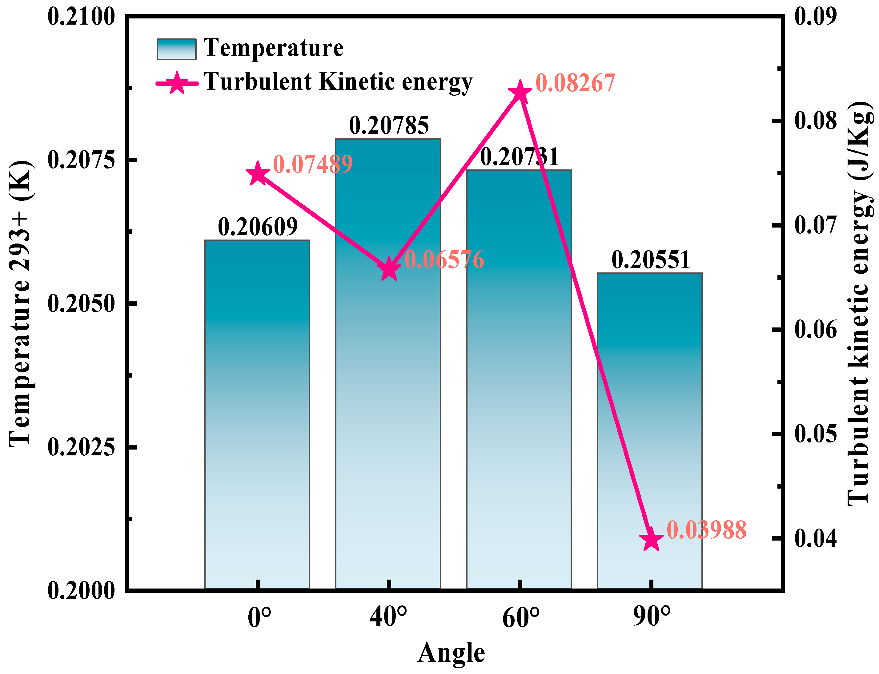
Figure 5 shows the trend of the influence of blade angle variation on temperature and turbulence energy. The overall temperature variation range is between 293.20551 K and 293.20785 K, with turbulent energy ranging from 0.03988 to 0.08267. As shown in the figure, the temperature shows a trend of first increasing and then decreasing with the increase in angle, while the turbulence energy shows a trend of first decreasing, then increasing, and then decreasing again. When the angle increases to 40°, the temperature inside the mixer reaches its highest value, while the turbulence energy decreases. The increase in temperature will affect the chemical composition of the feed, which is not conducive to ensuring the nutritional content of the feed. When the angle increases to 60°, the temperature decreases slightly, but the turbulence energy reaches its highest value. The change in angle causes a change in the area of the stirring blade in the vertical plane, thereby affecting temperature and turbulence energy, affecting temperature and turbulence energy. In addition, suitable temperature and good turbulence energy are conditions to ensure sufficient mixing of the feed. When the angle increases to 90°, the temperature and turbulence energy reach their lowest values, and poor turbulence energy is not conducive to the uniform mixing of the feed.

3.2. The Influence of Different Bottom Agitator Blade Sizes (M) on the Flow Field

To investigate the influence of the size (M) of the bottom agitator on the flow field, simulation experiments were conducted according to the design scheme in

Table 2. The size change of the bottom stirring blade.

Variable	M/mm	N/mm	C/°	R/pcs
1	40	35	60	4
2	45	35	60	4
3	50	35	60	4
4	55	35	60	4
5	60	35	60	4
6	65	35	60	4

. Among them, the top stirring blade size is fixed at 35 mm, the stirring blade angle is fixed at 60°, the number of stirring blades is fixed at 4, and the speed is fixed at 130 RPM/min.

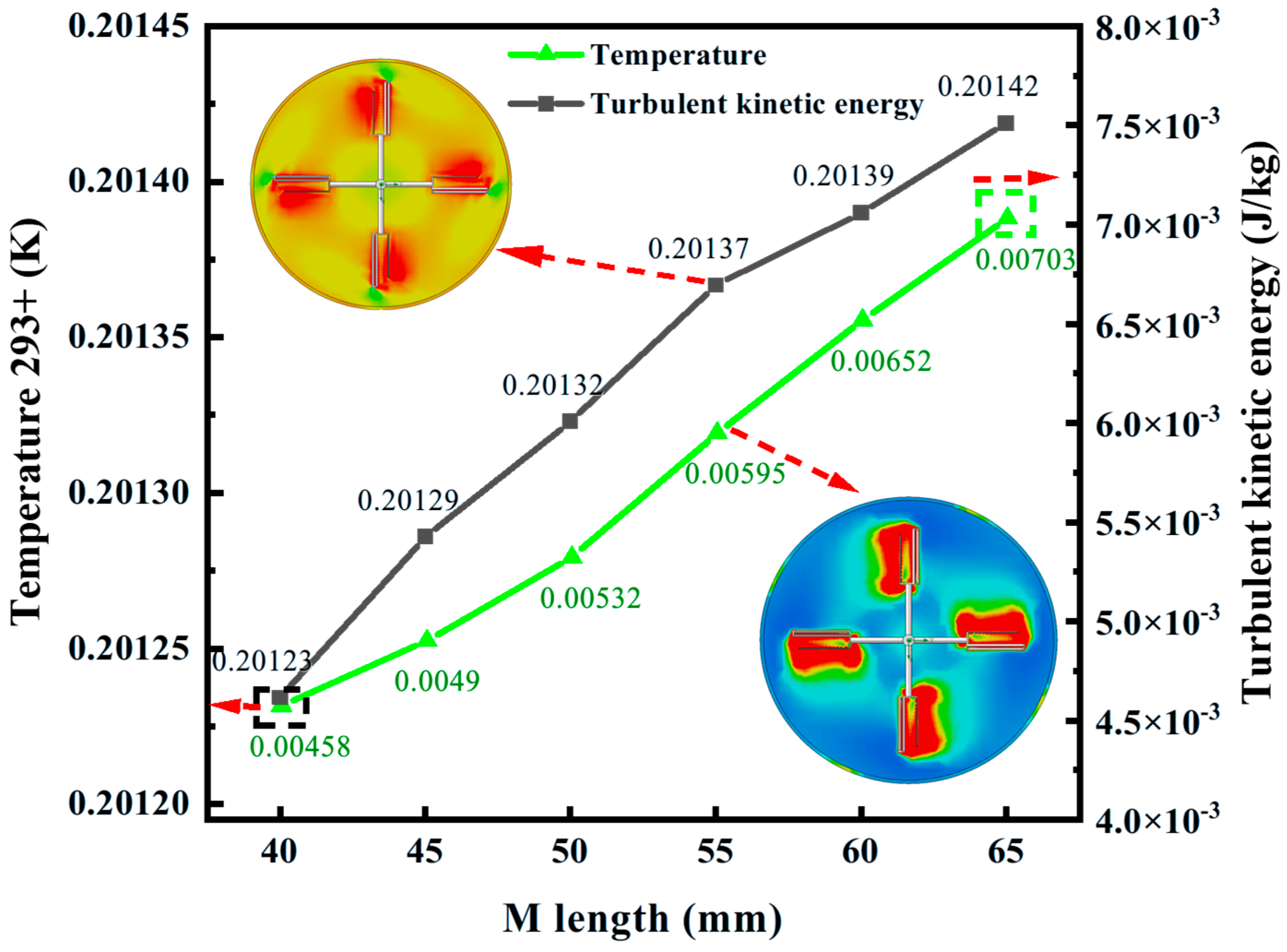
As shown in Figure 6, the black line represents the trend of temperature variation with the size of the bottom agitator blades, while the green line shows the change in turbulence energy. Overall, temperature and turbulence energy gradually increase as M increases from 40 mm to 65 mm. Specifically, as the size of the upper and lower agitator blades increases, the turbulence energy and temperature of the fluid also increase, indicating that larger sizes help enhance the mixing effect and heat accumulation of the fluid. Specifically, at M = 40 mm, the temperature is relatively low, around 293.20123 K, and the turbulence energy is also low, only 4.58 × 10⁻³ J/kg, indicating that the smaller size of the upper square edge accelerates the heat dissipation of the fluid in the mixer, and the fluid flow is relatively stable. As M increases to 45 mm, the temperature rises slightly, reaching 293.20129 K. This is due to changes in fluid flow characteristics, enhanced heat transfer, and increased turbulence energy, reaching 4.9 × 10⁻³ J/kg, indicating that fluid dynamics become more intense at this size, leading to improved mixing efficiency. As M increases to 50 mm, the temperature slightly rises to 293.20132 K, and heat transfer continues to increase. The turbulent kinetic energy has also increased, reaching 5.32 × 10⁻³ J/kg, and the mixing efficiency continues to improve. When further increased to M = 55 mm, the temperature continued to rise to 293.20137 K, and the heat accumulation of the fluid was significantly enhanced under the influence of larger edge sizes. The turbulent kinetic energy continues to rise to 5.95 × 10⁻³ J/kg, indicating that larger sizes can maintain good heat exchange effects. As M increases to 60 mm, the temperature steadily rises to 293.20139 K, showing a stable trend of heat accumulation. At the same time, the turbulence energy increased again, reaching 6.52 × 10⁻³ J/kg, indicating an increase in the complexity of fluid flow and an enhancement of turbulence. Finally, at M = 65 mm, the temperature reached its highest value of 293.20142 K, and the turbulent energy also reached a peak of 7.03 × 10⁻³ J/kg, indicating that the fluid flow was most intense at this time, and the mixing effect and heat exchange efficiency inside the mixer were the highest. The reason for this phenomenon is that a larger upper square edge size can effectively enhance the turbulence intensity of the fluid, making the mixing more uniform. At the same time, due to the enhancement of turbulence, the heat transfer and mixing efficiency of the fluid have been significantly improved.

In summary, increasing the size of the bottom agitator not only increases temperature and turbulence energy but also significantly improves mixing efficiency by enhancing turbulence and heat exchange. Especially at M = 65 mm, the mixing effect and heat conduction of the fluid reach their optimal state. This indicates that optimizing the design of the mixer, especially adjusting the blade size, can effectively improve the mixing efficiency and thus enhance the overall performance of the mixer.

3.3. The Influence of Different Top Agitator Blade Sizes (N) on the Flow Field

To investigate the influence of the size (N) of the top agitator on the flow field, simulation experiments were conducted according to the design scheme in

Table 3. Change the values of dimension N of the lower square port.

Variable	M/mm	N/mm	C/°	R/pcs
1	45	35	60	4
2	45	40	60	4
3	45	45	60	4
4	45	50	60	4
5	45	55	60	4
6	45	60	60	4

. Among them, the size of the bottom stirring blade is fixed at 45 mm, the angle of the stirring blade is fixed at 60°, the number of stirring blades is fixed at 4, and the speed is fixed at 130 RPM/min.

As shown in Figure 7, as the size of the top agitator blades increases from 35 mm to 65 mm, the temperature and turbulence energy generally show an upward trend. Specifically, as the blade size increases from 35 mm to 55 mm, the temperature steadily rises from 293.20116 K to 293.20136 K. This indicates that as the size of N increases, the temperature inside the system slightly rises, and the magnitude of the temperature change is relatively small. When the blade size increases from 5 mm to 60 mm, there is a significant increase in temperature. The larger the blade size, the higher the temperature, as the contact area between the blade and the fluid continues to increase. In addition, the turbulent energy continuously increases with the increase in the size of the top agitator blades. When the blade size increases from 35 mm to 50 mm, the turbulent energy steadily increases from 0.00468 J/kg to 0.00547 J/kg. However, as the blade size increased from 50 mm to 60 mm, the turbulent energy inside the entire mixer sharply increased, rising from 0.00547 J/kg to 0.00756 J/kg. The increase in size can significantly enhance turbulence energy and improve mixing efficiency, further promoting the balance of nutrients in the feed.

As shown in Figure 8, the size of the top agitator has a significant impact on the distribution of turbulent energy within the system. A larger size will enhance the intensity and complexity of fluid motion, thereby increasing turbulent kinetic energy. Due to the longer fluid motion path caused by larger dimensions, the flow within the system becomes more complex. In summary, increasing the size of the top agitator not only increases temperature and turbulence energy but also significantly improves mixing efficiency by enhancing turbulence and heat exchange. Especially when M = 60 mm, the mixing effect and heat conduction of the fluid reach their optimal state.

3.4. The Influence of Different Blade Numbers on the Flow Field

To investigate the effect of the number of agitators on the flow field, simulation experiments were conducted according to the design scheme in

Table 4. Change the values of the number of agitators.

Variable	M/mm	N/mm	C/°	R/pcs
1	45	35	60	2
2	45	35	60	3
3	45	35	60	4
4	45	35	60	5
5	45	35	60	6
6	45	35	60	7

. Among them, the bottom stirring blade size is fixed at 45 mm, the top stirring blade size is fixed at 35 mm, the stirring blade angle is fixed at 60°, and the rotation speed is fixed at 130 RPM/min.

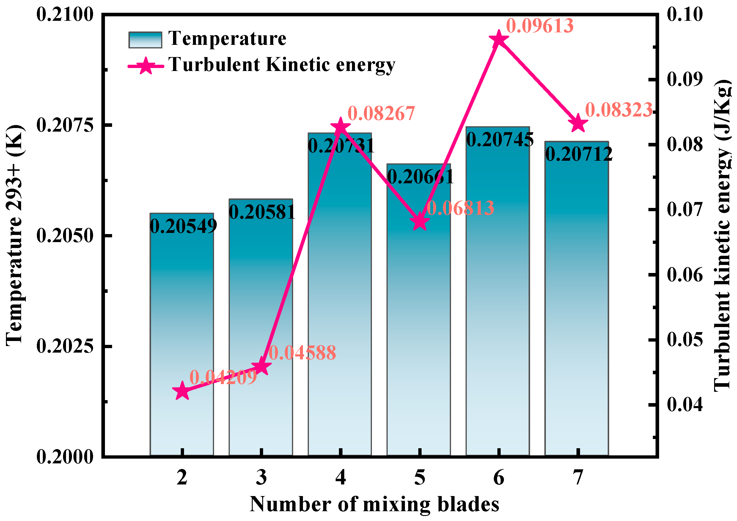
The observed non-monotonic trend in mixing efficiency with increasing blade count, as revealed by the flow field characteristics in Figure 9, can be attributed to a competition between two opposing hydrodynamic mechanisms. Under fixed speed conditions, appropriately increasing the number of impellers enhances fluid shear and overall disturbance, thereby improving flow field temperature and turbulence kinetic energy. Specifically, when using only 2 blades, the limited disturbance range and low mechanical energy input result in low fluid temperature (293.20549 K) and turbulent kinetic energy (0.04209 J/kg). As blades increase to 4, the significantly enhanced stirring effect converts more mechanical energy into heat through viscous dissipation while intensified shear generates more vortices, raising temperature to 293.20731 K and turbulent kinetic energy to 0.08267 J/kg—effectively promoting momentum/mass transfer and improving mixing efficiency.

However, beyond the optimal number (6 blades in this configuration), the flow dynamics become dominated by negative interference effects. When blades increase to 5, both temperature and turbulent kinetic energy decrease due to intensified flow interference and reduced channel space, manifested through: upstream blade wakes impacting downstream blades, reducing work efficiency; narrowed flow passages causing boundary layer separation and increased pressure resistance; and expanded friction surfaces converting more mechanical energy into thermal dissipation rather than generating effective turbulence. At 6 blades, the system reaches optimal performance (temperature 293.20745 K, turbulent kinetic energy 0.09613 J/kg) where blade arrangement balances shear surface expansion against flow blockage avoidance. Further increasing to 7 blades allows negative effects (flow blockage, wake interference, and friction loss) to dominate, significantly reducing mixing efficiency. This underscores the importance of optimizing blade geometry not just for maximizing shear but also for minimizing detrimental flow separation and inter-blade interference, highlighting the critical balance required between mixing enhancement and flow performance in mixer design.

In summary, there is an optimal value for the number of stirring blades (6 in this study). Moderate increase can improve mixing efficiency, but excessive increase can lead to a decrease in effectiveness due to deteriorating fluid dynamic conditions. This rule highlights the importance of balancing the relationship between mixing enhancement and flow performance in mixer design.

The study of agitator blade parameters in this research has brought significant practical engineering benefits. By optimizing the flow field and turbulence energy distribution, the mixing time has been effectively shortened, thereby significantly improving production efficiency and capacity. At the same time, the improved flow characteristics reduce local wear and vibration of the equipment, extend the service life of key components, and reduce maintenance costs. These advantages collectively enhance the comprehensive economy and operational sustainability of the mixing process.

4. The Influence and Optimization Based on the Response Surface Methodology

Considering the multiple influencing variables in this study’s experimental setup, conducting all possible experiments would significantly increase the number of trials and computational resources. Therefore, the Response Surface Methodology (RSM) can be used to minimize the number of experiments, saving time and resources. RSM is an advanced Design of Experiments (DOE) technique that helps to understand and optimize responses in greater depth [28].

4.1. Box–Behnken Design (BBD)

The process involves conducting experiments based on a predefined experimental design scheme to gather a set of data. This data is then used to fit a quadratic multivariate regression equation, modeling the relationship between factors and response values. Analysis of variance is subsequently performed on the regression equation to determine the optimal design scheme.

There are two main types of response surface designs: Central Composite Design (CCD) and BBD [29]. The central composite design often includes many design points that exceed the originally set levels, which may not be suitable when multiple levels are needed for comprehensive analysis. For the detailed factor analysis in this chapter, the BBD is chosen. All design points in the BBD remain within the safe operating region without any axial points. This ensures that all experiments are conducted within the defined safe boundaries.

4.2. Experimental Design Setup

Based on the previous single-factor simulation analysis, it has been observed that the internal structure of mixing blades significantly affects both turbulent kinetic energy and temperature within the fluid domain system. To further investigate the influence of blade structure on fluid characteristics and optimize the results, turbulent kinetic energy and fluid temperature will be used as response variables.

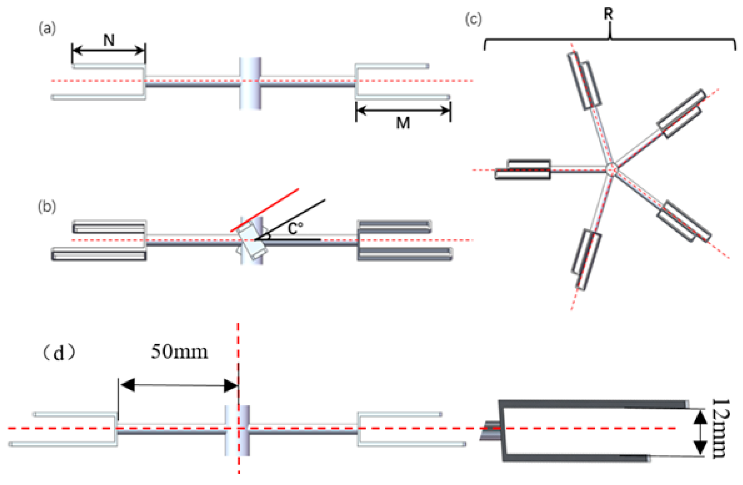
The factors selected for this response surface experiment are the upper-end square opening size (M), lower-end square opening size (N), blade angle (C), and number of blades (R). A four-factor with two response values of the response surface experiment will be designed. The goal is to identify the optimal combination that maximizes both turbulent kinetic energy and temperature within the fluid domain. The levels of experimental factors are presented in

Table 5. Setting factors and levels of the response surface.

Influence Factor	Variable	Low-Level	High-Level
Dimensions of the upper square port M (mm)	A	40	65
Dimensions of the lower square port are N (mm)	B	35	65
Blade angle (°)	C	0	90
Blade number (pcs)	D	2	7

.

A total of 29 experimental design schemes were generated through software analysis for simulation calculations in

Table 6. Parameters of DOE and the setting of the scheme.

Std	Run	Factor 1 A:M (mm)	Factor 2 B:N (mm)	Factor 3 C:C (°)	Factor 4 D:R (pcs)
1	22	40	35	45	5
2	10	65	35	45	5
3	8	40	65	45	5
4	7	65	65	45	5
5	25	52.5	50	0	2
6	18	52.5	50	90	2
7	15	52.5	50	0	7
8	21	52.5	50	90	7
9	14	40	50	45	2
10	29	65	50	45	2
11	3	40	50	45	7
12	17	65	50	45	7
13	27	52.5	35	0	5
14	28	52.5	65	0	5
15	2	52.5	35	90	5
16	26	52.5	65	90	5
17	6	40	50	0	5
18	1	65	50	0	5
19	24	40	50	90	5
20	5	65	50	90	5
21	11	52.5	35	45	2
22	4	52.5	65	45	2
23	16	52.5	35	45	7
24	23	52.5	65	45	7
25	13	52.5	50	45	5
26	19	52.5	50	45	5
27	20	52.5	50	45	5
28	9	52.5	50	45	5
29	12	52.5	50	45	5

. By analyzing the results of these 29 simulation experiments, mathematical models for fluid turbulent kinetic energy and fluid temperature were derived. The data obtained from these simulations were then subjected to regression and fitting, using a full quadratic polynomial to develop regression equations that describe the relationship between the factors and the response values.

4.3. Optimization Results Analysis

Based on the experimental design results, we can identify the constant term, linear terms (A, B, C, D), interaction terms (AB, AC, AD, BC, BD, CD), and quadratic terms (A², B², C², D²) that influence both fluid temperature and turbulent kinetic energy. The mathematical models, derived using coded factors, yield the following regression equations:

Turbulent Kinetic Energy = 0.0183 + 0.0007*A + 0.0009*B − 0.0036*C + 0.0026*D + 0.0001*AB − 0.0006*AC − 0.0006*AD − 0.0009*BC − 0.0004*BD − 0.0012*CD − 0.0057*A² − 0.0056*B² − 0.0043*C² − 0.0048*D².

Temperature = 0.2026 + 0.0002*A + 0.0001*B + 0.0004*D + 0.0003*AD + 0.0002*BD − 0.0005*A² − 0.0005*B² − 0.0008*C² − 0.0005*D².

To evaluate whether these models are suitable for optimization, significance tests and variance analysis were performed on the coefficients of the mathematical models. Figure 10 illustrates the actual versus predicted values of the simulation results for the target variable. Most data points cluster around the 45° line, suggesting a strong correlation between the actual and predicted values. The closer the response values of the established model are to the 45° line, the higher the model’s predictive accuracy [30]. In addition, key indicators such as the coefficient of determination (R²), adjusted-R², and predicted-R² were used to evaluate model suitability. R² Values: The R² values for turbulent kinetic energy and temperature are 0.9769 and 0.9683, respectively. Both values are close to 1, indicating a high degree of fit [31]. Adjusted-R² and Predicted-R² Differences: The differences between adjusted-R² and predicted-R² are 0.0778 and 0.0897 for turbulent kinetic energy and temperature, respectively. Both differences are less than 0.2, further confirming the model’s suitability. A variance statistical analysis was also conducted to validate the model, using metrics such as the p-value, F-value, and lack-of-fit value: a p-value of less than 0.05 indicates that the model is statistically significant. The analysis shows that the p-values for both models are all less than 0.05, confirming the statistical significance of the quadratic models [32]. F-value: A higher F-value indicates greater significance of the equation and a better fit. Both models show high F-values, demonstrating their significance. Lack-of-fit Value: A non-significant lack-of-fit value implies that the model is reliable and reasonable.

Table 7. Analysis of variance of the regression model.

Source	DOF	Turbulent Kinetic Energy		Significance	Temperature		Significance
		F	p		F	p
Model	14	42.37	<0.0001	**	30.53	<0.0001	**
A	1	5.07	0.0409	*	18.73	0.0007	**
B	1	8.46	0.0114	*	13.53	0.0025	**
C	1	127.91	<0.0001	**	0.7233	0.4094	×
D	1	67.68	<0.0001	**	94.49	<0.0001	**
AB	1	0.0578	0.8135	×	0.0851	0.7748	×
AC	1	1.29	0.2745	×	0.0668	0.7998	×
AD	1	1.26	0.2805	×	11.85	0.0040	**
BC	1	2.72	0.1215	×	0.4641	0.5068	×
BD	1	0.4545	0.5112	×	8.35	0.0119	*
CD	1	4.99	0.0424	*	0.1962	0.6645	×
A2	1	177.25	<0.0001	**	65.82	<0.0001	**
B2	1	173.65	<0.0001	**	73.87	<0.0001	**
C2	1	99.90	<0.0001	**	198.22	<0.0001	**
D2	1	127.22	<0.0001	**	77.35	<0.0001	**
Residual	14	-	-	-	-	-	-
Misfit	10	3.93	0.0996	-	1.40	0.3987	-
Pure error	4	-	-	-	-	-	-
Cor total	28	-	-	-	-	-	-

Note: * in the table indicates a significant difference (p < 0.05); ** was very significant (p < 0.01); There was no significant difference in × (p > 0.05); - was a placeholder, meaning there was no data here.

presents the analysis results, demonstrating that the response surface models for both turbulent kinetic energy and temperature are accurate and effective. The significant terms for each model are as follows: Turbulent Kinetic Energy: Significant terms include A, B, C, D, CD, A², B², C², and D². Temperature: Significant terms include A, B, D, AD, BD, A², B², C², and D². These findings indicate that both models are well-suited for predicting and optimizing the turbulent kinetic energy and temperature in the fluid domain system based on the chosen design parameters. The use of these models can significantly enhance the understanding and optimization of flow characteristics and mixing performance in the feed mixer, leading to improved efficiency and effectiveness in practical applications.

4.3.1. Response Surface Analysis

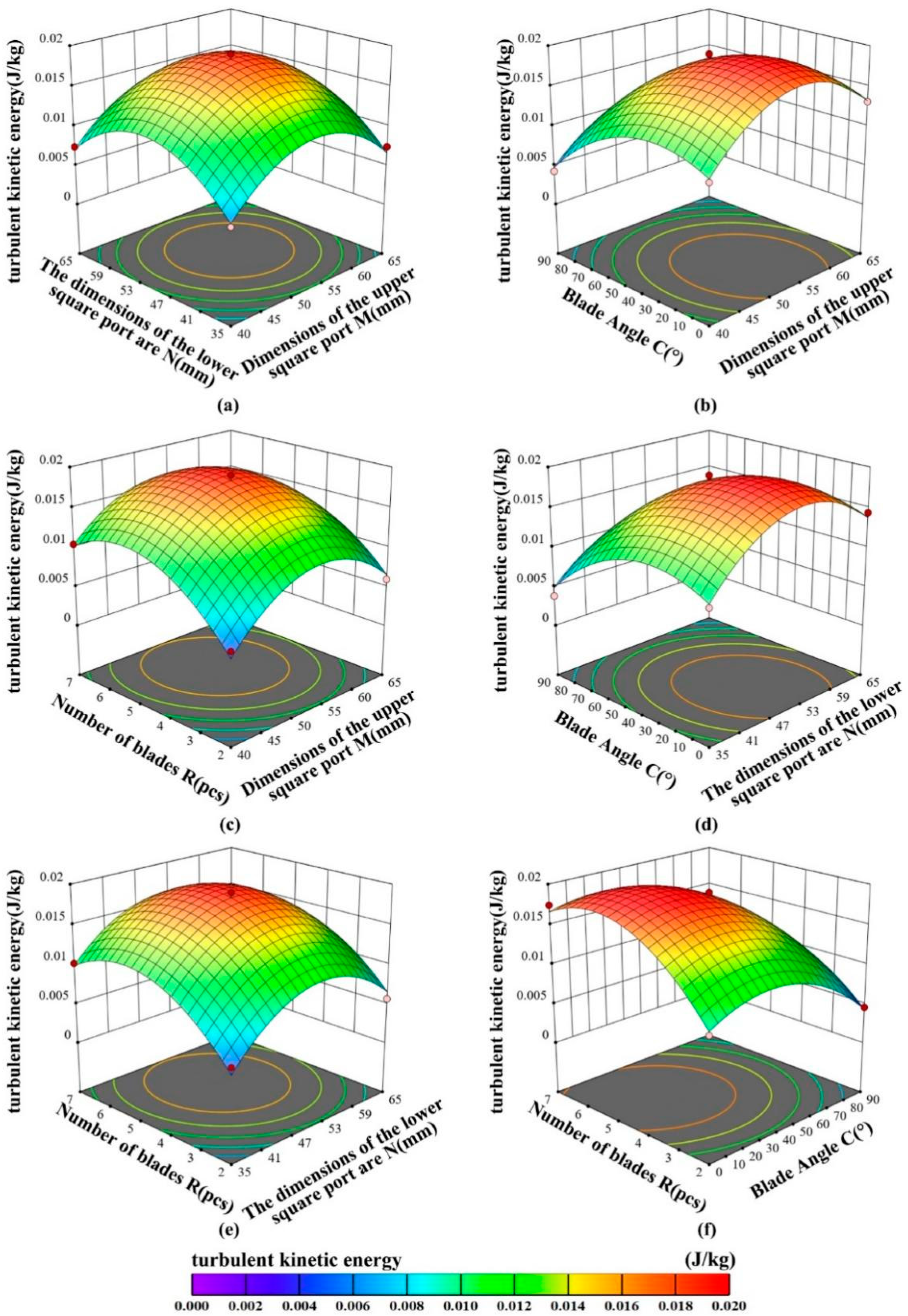
Figure 11a–f presents three-dimensional response surfaces and two-dimensional contour plots illustrating the effects of different decision variables on turbulent kinetic energy. These plots, based on simulated calculations, help assess the interactions between independent variables and their influence on the turbulent kinetic energy.

The analysis ranks the significance of the four factors (upper port size M, lower port size N, blade angle C, and number of blades R) on turbulent kinetic energy as follows, from most to least significant: Blade Angle C > Blade Number R > Upper Port Size M > Lower Port Size N. Among these factors, blade angle (C) has the most pronounced effect on turbulent kinetic energy. Adjusting the blade angle significantly impacts turbulent kinetic energy, followed by the number of blades, the upper port size, and finally, the lower port size.

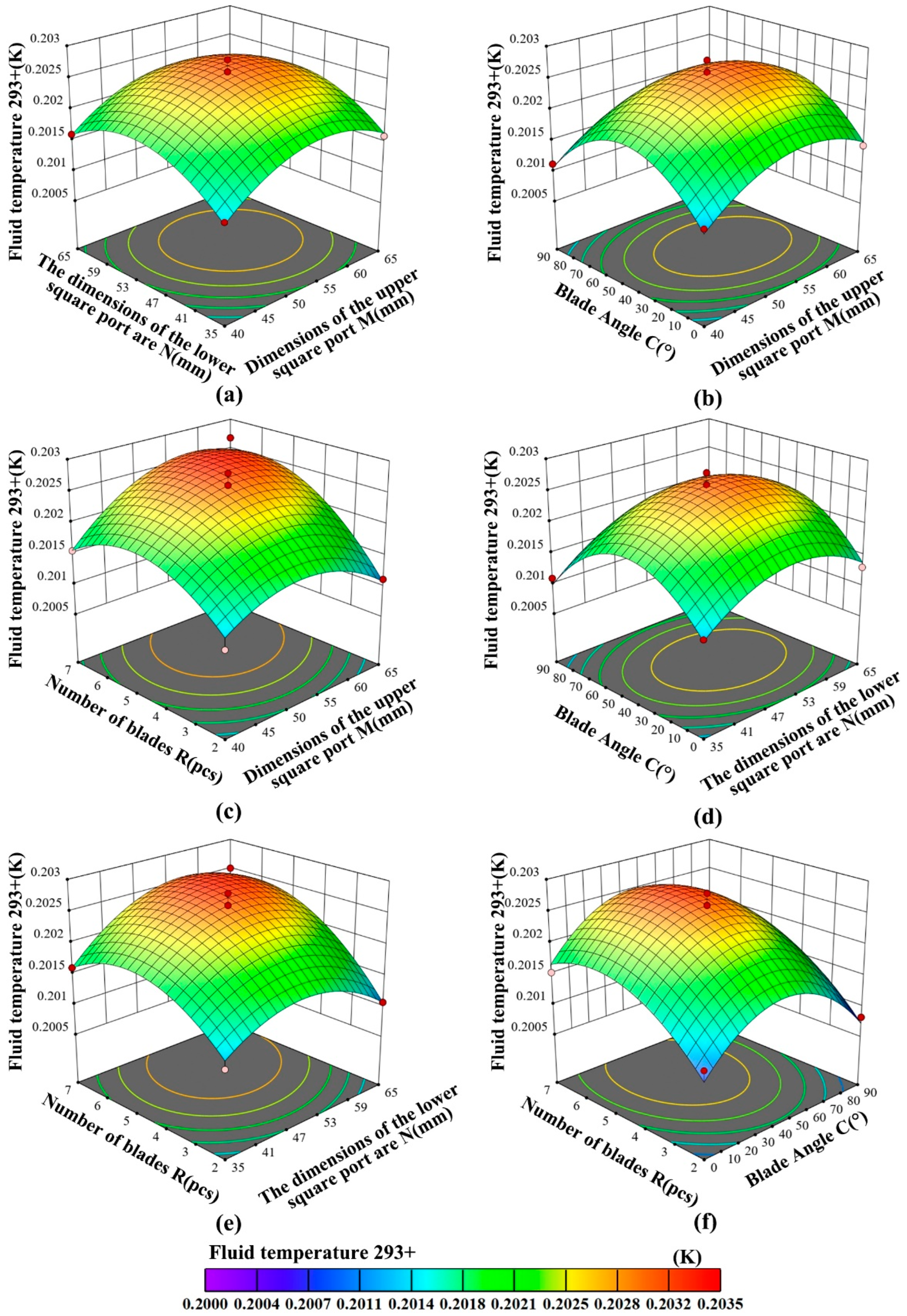
Figure 12 illustrates the impact of different decision variables on fluid temperature. The trends of the curves and the surface angles reflect the influence of each variable on fluid temperature. Figure 11a indicates that fluid temperature gradually increases with the size of the upper opening (M) and lower opening (N), suggesting a positive correlation between these factors and fluid temperature. Figure 11b,c,e demonstrate that the number of blades (R) and the size of the upper opening (M) significantly affect fluid temperature, whereas the size of the lower opening (N) has less impact. The importance of these factors on fluid temperature, ranked from highest to lowest, is as follows: 1. Number of blades (R), 2. Upper opening size (M), 3. Lower opening size (N), 4. Blade angle (C). The number of blades (R) has the most significant influence on fluid temperature, followed by the size of the upper opening (M), the size of the lower opening (N), and finally the blade angle (C).

4.3.2. Optimal Response Surface Prediction and Validation

The primary objective of optimization is to identify the best conditions for maximizing turbulent kinetic energy and fluid temperature in the fluid domain system. Optimal conditions are determined based on each factor’s settings relative to the response variables.

Table 8. Optimization combination of the response surface method.

Case	A:M (mm)	B:N (mm)	C:C (°)	D:R (pcs)	Response Value 1	Response Value 2
Case 0 (Traditional parameters)	45	35	60	4	0.00468	0.20116
Case 1 (Only turbulent kinetic energy considered)	50.3	49.3	31	5	0.01904	0.20247
Case 2 (Fluid temperature only)	56.7	54.0	45	6	0.01764	0.20278
Case 3 (Optimal combination of turbulent kinetic energy and fluid temperature)	54.9	52.5	39	5	0.01900	0.20274

shows the optimal combination of Case 1 (considering only turbulent kinetic energy), Case 2 (considering only fluid temperature), and Case 2 (considering both turbulent flow energy and fluid temperature). In Case 3, the turbulent kinetic energy (response value 1) is 0.01900 J/kg, slightly less than 0.01904 J/kg in Case 1. The fluid temperature (response value 2) in Case 3 is 0.20274 K, marginally lower than 0.20278 K in Case 2. Given the minimal differences, Case 3 is selected as the optimal combination, where the upper square mouth dimension (M) is 54.9 mm, the lower square mouth dimension (N) is 52.5 mm, the blade angle (C) is 39°, and the number of blades (R) is 5. These conditions lead to more uniform mixing.

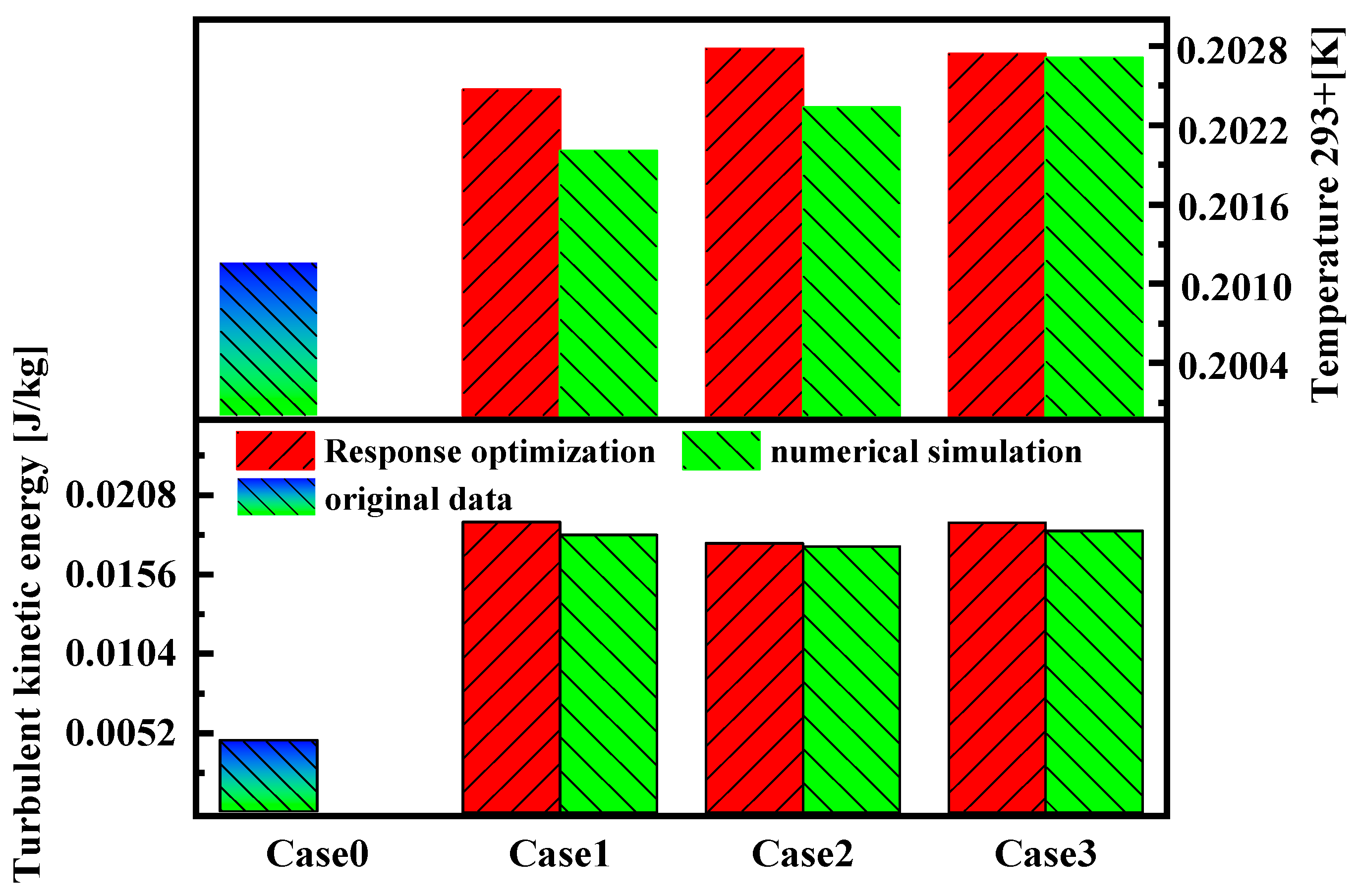
Figure 13 compares the optimization prediction results and simulation results for Case 0, Case 1, Case 2, and Case 3. The differences between the optimized prediction results and simulation results for turbulent kinetic energy are 4.41%, 1.13%, and 2.94% for Case 1, Case 2, and Case 3, respectively. For fluid temperature, the differences are 0.22%, 0.22%, and 0.06%. These errors are within acceptable ranges, validating the response surface optimization results. The optimized turbulent kinetic energy and fluid temperature are approximately 67% and 7% higher, respectively, compared to Case 0.

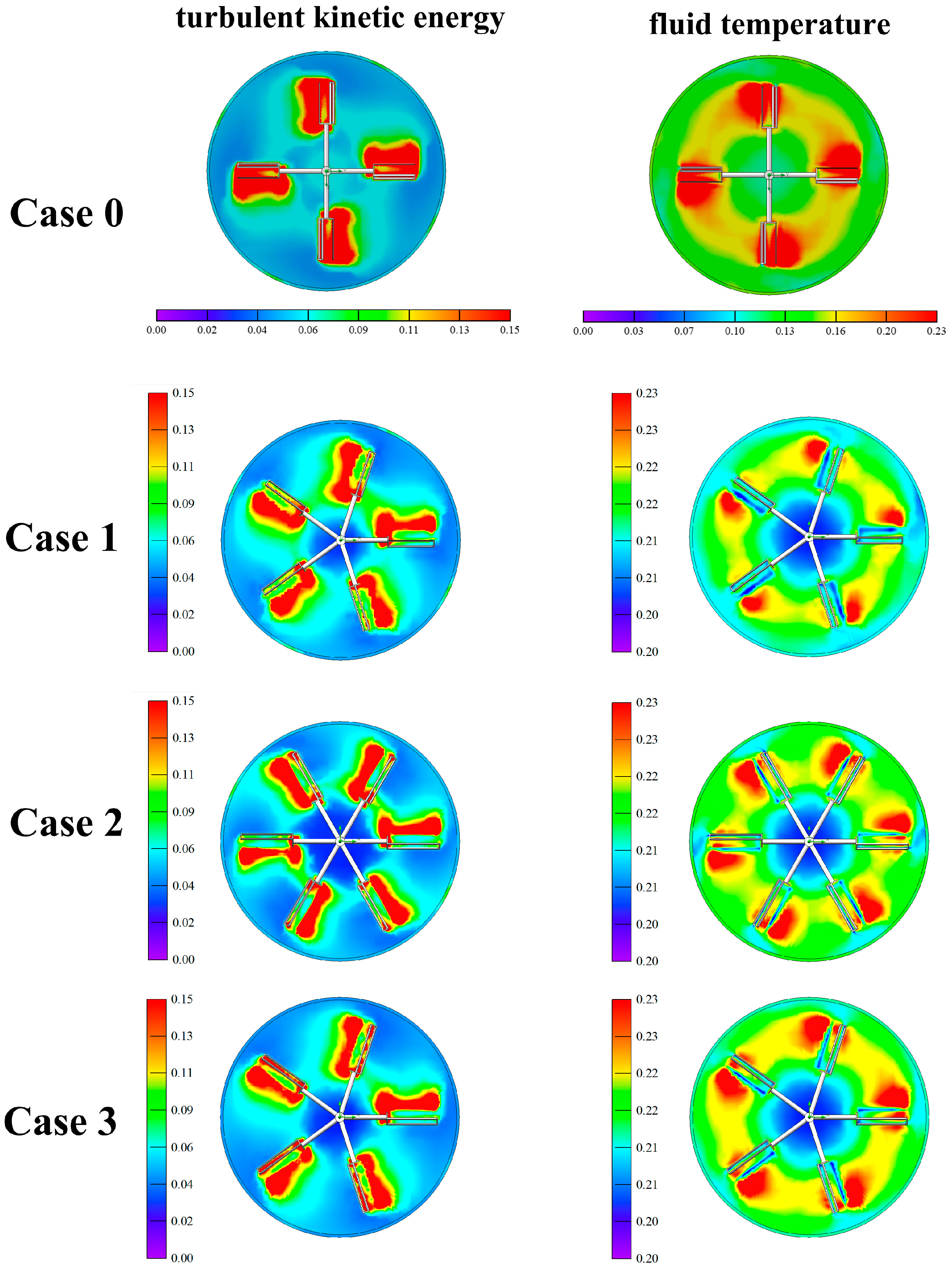
Figure 14 shows the distribution of turbulent kinetic energy and fluid temperature in the fluid domain system for Case 0, Case 1, Case 2, and Case 3. In Case 3, the turbulent kinetic energy contour map shows more dispersed and higher-value red regions compared to Case 0. In the fluid temperature map, Case 3 shows red and yellow regions more evenly distributed in higher-value areas, indicating improved mixing performance.

5. Summary

Optimizing feed mixers by modifying the internal structure of stirring paddles to achieve optimal mixing uniformity has been a longstanding objective for researchers. This paper employs computational fluid dynamics numerical simulations to analyze and evaluate the turbulent kinetic energy and fluid temperature distribution within the fluid domain. The primary conclusions drawn from this study are as follows:

(1) Generally, an increase in the upper port size (M) and the number of blades (R) leads to an enhancement in turbulent kinetic energy and fluid temperature. However, an inflection point is observed when M reaches 50 mm, which may be attributed to fluid redistribution effects. With an increasing number of blades (R), the turbulent kinetic energy and fluid temperature exhibit a non-linear trend—initially increasing, then decreasing, and subsequently rising again—suggesting that identifying an optimal value for a single factor is challenging.

(2) The regression models were rigorously validated using multiple statistical metrics, including R², adjusted R², predicted R², p-values, F-values, and lack-of-fit tests, all of which demonstrated high predictive accuracy and adaptability. Analyzing parameter interactions revealed the following rankings of influence on turbulent kinetic energy: blade angle (C) > number of blades (R) > upper square aperture (M) > lower square aperture (N). For fluid temperature, the order of influence was: number of blades (R) > upper square aperture (M) > lower square aperture (N) > blade angle (C).

(3) Response surface optimization identified Case 3 as the optimal configuration compared to Case 1. At a rotational speed of 130 RPM, Case 3 exhibited a 75% increase in turbulent kinetic energy relative to Case 0 (with an actual simulated increase of 67%). Additionally, fluid temperature increased by 7.8% (with an actual simulated rise of 7.7%).

The findings of this study demonstrate that optimizing the internal structure of the impeller significantly enhances the performance of the fluid domain. The optimized impeller design effectively increases turbulent kinetic energy, promoting a more dynamic and uniformly distributed fluid mixture. This enhancement not only improves fluid temperature stability but also substantially enhances mixing uniformity. Such improvements have far-reaching implications for industrial applications requiring high-precision and high-efficiency mixing, particularly in complex multiphase systems such as chemical reactors, pharmaceutical production, food processing, and feed blending.

Although this study has yielded instructive optimization outcomes through CFD numerical simulation, a series of critical tasks remain to be addressed to facilitate its transition to practical industrial applications. Future research should prioritize the industrial scaling of these achievements, building upon experimental validation. Subsequent efforts should focus on scaling the optimized impeller design to industrial-scale mixers in accordance with principles of geometric and dynamic similarity, while investigating potential scale effects that may emerge during the amplification process. This will ensure the preservation of performance advantages in large-scale equipment, ultimately achieving the overarching goals of energy conservation and consumption reduction. Lastly, the methodology developed in this study demonstrates significant potential for broad applicability. The proposed optimization framework may be extended to feed types with diverse physical properties, such as high-viscosity molasses-added feed, fiber-rich forage, or premixed micro-ingredients with substantial density variations. Investigating whether the optimal impeller configuration varies with material characteristics will pave the way for developing adaptive, high-efficiency next-generation intelligent mixing equipment with comprehensively optimized performance.