Abstract
Drilling fluid loss is a common and complex downhole problem that occurs during drilling in deep fractured formations, which has a significant negative impact on the exploration and development of oil and gas resources. Establishing a drilling fluid loss model for the quantitative analysis of drilling fluid loss is the most effective method for the diagnosis of drilling fluid loss, which provides a favorable basis for the formulation of drilling fluid loss control measures, including the information on thief zone location, loss type, and the size of loss channels. The previous loss model assumes that the drilling fluid is driven by constant flow or pressure at the fracture inlet. However, drilling fluid loss is a complex physical process in the coupled wellbore circulation system. The lost drilling fluid is driven by dynamic bottomhole pressure (BHP) during the drilling process. The use of a single-phase model to describe drilling fluids ignores the influence of solid-phase particles in the drilling fluid system on its rheological properties. This paper aims to model drilling fluid loss in the coupled wellbore–-fracture system based on the two-phase flow model. It focuses on the effects of well depth, drilling pumping rate, drilling fluid density, viscosity, fracture geometric parameters, and their morphology on loss during the drilling fluid circulation process. Numerical discrete equations are derived using the finite volume method and the “upwind” scheme. The correctness of the model is verified by published literature data and experimental data. The results show that the loss model without considering the circulation of drilling fluid underestimates the extent of drilling fluid loss. The presence of annular pressure loss in the circulation of drilling fluid will lead to an increase in BHP, resulting in more serious loss.
1. Introduction
Drilling fluid loss refers to the phenomenon that drilling fluid enters the formation through fractures under the effect of overbalanced pressure in drilling [1]. In the process of well construction in naturally fractured formations, frequent loss of drilling fluid not only consumes drilling fluid and a large amount of lost circulation materials, resulting in serious economic losses, but also increases non-productive time, lengthens the cycle of well construction, and seriously delays the exploration and development process [2]. Drilling fluid loss is also the most serious form of formation damage during the drilling and completion stage. It damages oil and gas well productivity, reduces reservoir production capacity and single-well yield, and is even more likely to cause complex downhole accidents, such as stuck pipes, borehole collapse, or well control issues. It is one of the engineering and technical problems that have long constrained safe and efficient drilling of deep and ultra-deep wells. Therefore, effective control of drilling fluid loss in deep fractured formation is particularly important [3,4,5,6,7].
Understanding the mechanisms and patterns is central to addressing the issue of drilling fluid loss [8,9]. Scholars globally have proposed diverse models for preventing and mitigating drilling fluid losses. Models vary by their considerations of fracture properties and drilling fluid rheology, such as fracture deformation and wall surface roughness [10,11], drilling fluid rheological behavior [12,13], fracture wall filtration characteristics [14], 2D discrete fracture network [15,16], induced fracture dynamic propagation characteristics [17], and 3D discrete fracture in complex formations [18]. Building upon this foundation, some researchers have established fracture–vuggy drilling fluid loss models incorporating both non-Darcy flow and Darcy flow [19,20]. Studies on fluid loss models for drilling mud within single fractures in fractured formations have a history of several decades. Early research employed simplified modeling based on Darcy’s law under steady-state conditions [21,22]. Dyke et al. (1995) found that drilling fluid loss velocity within fractures exhibits an initial increase followed by a decrease, and the decline in loss velocity is associated with rising fluid pressure within the fracture [23]. Zimmerman and Bodvarsson (1996) established a flow model for single-phase fluid within rough fractures, building upon the Navier–Stokes equations, and provided a derivation of the cubic law as a solution for the model [24]. Lietard et al. (1996) proposed a lost circulation model for Bingham fluid within undeformable, infinitely long smooth fractures [25]. By solving this model, curves depicting drilling fluid invasion depth versus time under varying fracture widths were obtained; subsequently, the width of the loss fracture was derived by matching field drilling fluid loss curves with these theoretical curves. Based on the theory advanced by Lietard (1996), the eventual cessation of drilling fluid loss was attributed to the fluid’s rheological properties [25]. Sanfillippo et al. (1997) established a lost circulation model for Newtonian fluid within one-dimensional infinitely long fractures, positing that the eventual cessation of loss was due to the plugging effect exerted by solid particles within the drilling fluid system on the fractures [26]. Lavrov and Tronvoll (2004) considered fracture propagation during drilling fluid loss, introduced the theory of linear elastic fracture deformation, and established lost circulation models for Bingham and power-law fluids within finite-length, one-dimensional radial fractures [27]. Compared with prior drilling fluid loss models, these incorporated the fluid-loss effect through fracture walls driven by the differential pressure between the fluid pressure in the fracture and the formation pressure, and further accounted for the influence of fracture dip angle on both the fluid loss rate and cumulative loss volume. Li et al. (2014), based on the genetic mechanisms of fluid loss fractures, proposed a new classification methodology for fracture-induced losses and developed corresponding lost circulation pressure models [28]. Additionally, they established lost circulation models for Herschel-Bulkley (H-B) fluid within one-dimensional linear fractures, two-dimensional planar fractures, and three-dimensional fracture networks, introducing the theory of power-law fracture deformation to analyze the impact of fracture deformation behavior on fluid loss dynamics. However, these models do not incorporate fracture surface roughness and fracture wall fluid loss, exhibiting certain limitations. Feng and Gray (2018) utilized ABAQUS software to couple drilling fluid circulation within the wellbore with fracture propagation during fluid loss, enabling dynamic prediction of loss volume and fracture geometry throughout drilling operations [17]. Pang et al. (2019) established multiphase solid–liquid flow equations for two-dimensional rough, non-deformable fractures based on computational fluid mechanics principles [29]. Rami Albattat and Hussein Hoteit (2019, 2021) identified minor fracture wall deformation during fluid loss as a primary cause of inaccuracies in existing dynamic loss models [30,31,32]. These models also lack established relationships between the mud invasion front, intra-fracture pressure differential, and drilling fluid rheological properties. By incorporating non-parallel fractures into power-law fluid loss equations, they evaluated the impact of fracture heterogeneity along the length on drilling fluid loss behavior. Lost circulation characteristic curves serve as the most common diagnostic method for fluid loss, operating on the principle that dynamic loss behavior responds to overbalance pressure, fracture geometric and mechanical properties, and drilling fluid performance. Current research on dynamic fluid loss behavior primarily focuses on single fractures and has yet to incorporate the effects of annular frictional pressure losses during drilling fluid circulation on such behavior.
Drilling fluid loss refers to a multi-physical process in which the drilling fluid, being a complex two-phase fluid containing a high concentration of solid particles, losses into the formation through fracture channels in the coupled drill tool–wellbore–fracture system under specific engineering parameters. The distribution effect of the solid phase on the behavior of drilling fluid loss cannot be ignored. To address the above issues, a three-dimensional drilling fluid loss model coupling drill tools, wellbores, and fractures was established. The finite volume method was used for solving, comprehensively exploring the effects of thief zone depth, drilling fluid performance, drilling displacement, and fracture geometry on the behavior of drilling fluid loss, to better understand the mechanisms and patterns of drilling fluid loss in deep fractured formations. With the diagnosis of drilling fluid loss as the core, the connection between drilling fluid loss parameters and engineering response characteristics was clarified, thereby constructing a framework for drilling fluid loss diagnostic technology.
2. Methodology
Drilling fluids are complex multiphase systems composed of a liquid phase and a high concentration of solid-phase particles, which mainly include bentonite, barite, cuttings and other common treatments in drilling fluid. The solid-phase content of drilling fluid is usually 20–40%, and the size of these solid-phase particles is usually less than 100 μm, which are uniformly dispersed in the drilling fluid. Therefore, the loss problem of drilling fluid within the coupled wellbore–fracture system is a typical multiphase flow problem. Common multiphase flow models mainly include the Euler–Euler model and the Euler–Lagrange model [33]. The Euler–Lagrange model mainly focuses on tracking the trajectory of a single particle and the change in its surrounding flow field, and the interactions between the microscopic properties of a single particle, particle–particle, particle–fluid, and particle–boundary are non-negligible for two-phase flow behavior. In contrast, in the Euler–Euler model, both the liquid and solid phases are regarded as continuous fluids, the two phases are interspersed with each other, the influences of the distribution effect of the highly concentrated solid phase on the two-phase flow behavior are considered, and the monitoring of the two-phase flow behavior is realized through the calculation of the local flow field. In the study of drilling fluid loss behavior at the formation scale, the velocity and pressure response in the computational unit are the information we pay close attention to, while the solid-phase particles in the drilling fluid are small, and the trajectory of a single particle is difficult to be monitored and is not the main object of this study; therefore, using the Euler–Lagrange method will increase the redundancy of the computation. Therefore, in this paper, the Euler–Euler method is used to numerically simulate the drilling fluid loss within the coupled wellbore–fracture system.
2.1. Governing Equation
In the Two-Fluid Model, both the discrete and continuous phases are described by the Navier–Stokes equations, and the momentum transfer between the interfaces is modelled using the model [34,35,36].
During drilling fluid circulation and loss, there is no mass exchange between the solid and liquid phases, and the mass conservation equation for the liquid phase is expressed as:
where is the volume fraction of the liquid phase, %; is the density of the liquid, g/cm3; and is the velocity of the liquid, m/s. The mass conservation equation for the solid phase is given as
where is the volume fraction of solid phase, %; is the density of the solid, g/cm3; and is the velocity of the solid, m/s. As the volume fraction indicates the proportion of space occupied by each phase, the volume fraction of the liquid and solid must satisfy:
The conservation of momentum equation for the liquid is expressed as
where represents the acceleration of gravity, m/s2; is the drag coefficient between the liquid–solid phases, dimensionless; and is the stress tensor of liquid, Pa; which can be given as
where represents the shear viscosity of liquid, Pa·s; and is the unit vector, dimensionless. The conservation of momentum equation for the solid is expressed as [37]:
where is the pressure of solid, MPa; is the coefficient of traction between the liquid and the solid, and denotes the force tensor of the solid, Pa; expressed by [38]:
where is the dynamic viscosity, Pa·s; and is the shear viscosity, Pa·s. and can be given as [39]:
where is the radial distribution function of solid phase, dimensionless. When the solid concentration increases, can be used to correct the probability of collision before. is the particle size of solid, mm; is the elastic recovery coefficient between the solid particles, dimensionless; and is the proposed temperature of the particles, °C; expressed as [40]:
where is the energy generated by the force tensor of the solid, N·m; is the diffusion of energy, m2/s; is the diffusion coefficient, m2/s; is the collisional dissipation of energy, W/m3; is the energy exchange between the liquid, W; and solid phases, and is the solid pressure. In the Eulerian–Eulerian two-fluid model for CFD multiphase flows, the solid-phase pressure is introduced as a constitutive relationship into the momentum equation of the particle phase; its formulation derives from granular kinetic theory and serves as the key physical quantity characterizing normal stresses within the particle phase arising from inter-particle collisions and momentum transfer. This term closes the stress tensor in the particle phase momentum equation, directly influencing numerical stability and physical fidelity, while reflecting the “fluid-like” pressure effects induced by collisions, fluctuations, and friction within the particle collective. can be given as [41]:
Turbulence is an ideal flow state during drilling fluid circulation, which is conductive to improving the rock-carrying capacity of drilling fluid. The main turbulence models used for the simulation of solid–liquid flow process include the Spalart–Allmaras model, the model, the model and the Reynolds stress model. The standard model is used to calculate the turbulent viscosity of drilling fluid based on the requirements of high accuracy, simplicity of application, time-saving, and generality, where is the turbulent kinetic energy, m2/s2; and is the dissipation rate, m2/s3. The transport equations of and are expressed as [42,43]:
where , , and are constants and = 1.44, = 1.92. and are the turbulent Rump numbers for k and , respectively, which take the values = 1.0 and = 1.3. is the turbulent kinetic energy due to the mean velocity gradient, W/m3; is the effect of compressible turbulent pulsation expansion on the overall dissipation rate, W/m3; and is the turbulent viscosity coefficient, dimensionless. , , and are expressed as follows:
where is a constant and = 0.09.
The vast majority of drilling fluids are non-Newtonian fluids, for which several rheological models are proposed. The Herschel–Bulkely model adds an additional term to the power-law model, and is therefore a three-parameter rheological model. This model combines the advantages of the Bingham and power-law models and is more accurate than Bingham and power-law models in describing the rheological properties of drilling fluids over a wide range of shear rates. The intrinsic equation of H-B fluid is given as [44]:
where denotes the dynamic shear of the model, n is the flow pattern index, dimensionless; and K is the consistency factor of the drilling fluid, Pa·sn.
In the simulation of liquid–solid two-phase flow, the Euler–Euler model used is to assume that the dispersed phase is a continuous medium capable of interpenetration. The interaction forces and momentum interactions between the liquid and solid phase are mainly reflected in the traction forces between the liquid and solid, and the accurate choice of the traction model can be a more accurate application of numerical simulation. Common traction models are the Schiller–Naumann model, the Wen–Yu model, the Symmetric model, the Gidaspow model, and the Syamlal–O’Brien model. The Gidaspow model is a combination of the Wen–Yu model and Ergun model, which has been found to be more widely used in the study of liquid–solid two-phase flows and is suitable for most fluidization calculations. Therefore, the Gidaspow model is mainly used in this paper. The Gidaspow model can be given as [45]:
where is the resistance factor, dimensionless; which can be expressed as [46]:
where is the solid-phase Reynolds number, dimensionless; which can be given as
2.2. Physical Model and Simulation Conditions
Taking the tight sandstone formation in Ordos Basin as an example, it is mostly developed with shear tectonic fractures that extend along the tendency and strike for a long distance and are more stable in morphology. Based on imaging logging technology and combined with the description of fractures in field outcrops and cores, it is analyzed that the tight sandstone formation in Ordos Basin mainly develops high-angle fractures, and more than 90% of fractures have inclination angles greater than 75°. Therefore, vertical flat fractures are used in the simulation instead of real fractures, and the physical model is shown in Figure 1, considering drilling fluid circulation.
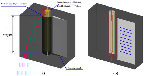
Figure 1.
Physical modeling of natural fracture in coupled wellbore system: (a) physical model of coupled pipe–wellbore–fracture system; (b) schematic diagram of drilling fluid flow process.
As shown in Figure 2, the quantitative characterization results of the fractures show that most of them are less than 1 m in height, mainly developing between 0 and 50 cm, with a peak height of about 10 cm. Most of the fracture widths are distributed in the interval of 0–5 mm, where the peak width is 2 mm. The geometric parameters of the fractures in the simulation are arranged as shown in Table 1.
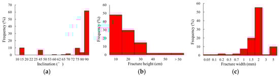
Figure 2.
Quantitative characterization of fractures in tight sandstone formations in Ordos Basin: (a) distribution of fracture inclination; (b) distribution of fracture height; (c) distribution of fracture width.

Table 1.
Fracture geometry parameters used in simulation.
At the inlet, a specified fluid velocity is applied according to the actual drilling pumping rate on site. After reaching the bottom of the well through the rotating drill pipe, some of the drilling fluid is lost into the formation through fractures, while the rest of the drilling fluid is returned to the ground through the annulus to simulate the real drilling circulation and loss process. The fracture outlet is considered a constant-pressure outlet with a value equal to the formation pore pressure. The drill pipe surface, wellbore, and fracture wall are all no-slip walls, and irregular undulations and friction of the wellbore and fracture wall are simulated by setting roughness constants. As drilling fluid is an incompressible fluid, its density remains constant. Fluid–particle and particle–particle heat transfer are not considered in this simulation. The spatial dispersion of the convective term in the equation is solved using a first-order windward scheme and the time integral is solved using a first-order implicit scheme. In this calculation, the CFD time step size is 1 × 10⁻² s. In this model, particle shape is generalized to spherical with uniform particle size, and detailed parameters used in this simulation work are shown in Table 2.
Table 2.
List of parameters used for simulation.
2.3. Model Validation
To validate the reliability of numerical simulations, this study utilized a multiphase flow migration experimental apparatus with a coupled wellbore–fracture system for lost circulation testing. The apparatus features a wellbore diameter of 150 mm and a length of 1.5 m, comprising three integrated modules: wellbore–fracture coupling module, mud preparation–pumping integration module, and unified control–data-acquisition module. The fracture module contains parallel vertical fractures with a length of 1 m, height of 30 cm, and an adjustable width range of 0–10 mm. Physical and schematic diagrams of the apparatus are shown in Figure 3.
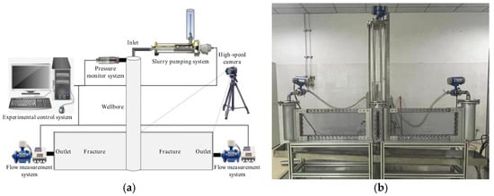
Figure 3.
Multiphase flow migration experimental apparatus with a coupled wellbore–fracture system: (a) Schematic diagram; (b) experimental apparatus.
Water was employed as the testing medium with a density of 0.998 g/cm3 and viscosity of 1.01 mPa·s. Specific experimental and simulation conditions are detailed in Table 3. To mitigate operational errors inherent in single-group tests, lost circulation tests were conducted at three distinct flow rates, thus obtaining BHP and drilling fluid loss rate within the coupled wellbore–fracture system under varying flow conditions. Experimental data were compared with the simulation results, as shown in Figure 4. The close agreement between simulated and experimental loss data (maximum error = 7.26%) validates the reliability and accuracy of the model calculations.
Table 3.
Comparison of experimental and simulation conditions.
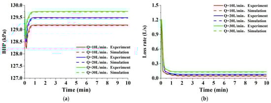
Figure 4.
Comparison between numerical simulation and experimental results under different pumping rates in a coupled wellbore–fracture system: (a) BHP; (b) drilling fluid loss rate.
3. Results and Discussions
3.1. Drilling Fluid Loss in Natural Fracture
The loss of drilling fluid is essentially the flow behavior of a non-Newtonian two-phase fluid composed of high-concentration solid particles and a liquid phase under pressure. The rate of drilling fluid loss is the manifestation of the flow speed of drilling fluid in the fracture per unit time. According to the simulation results, this article divides the process of natural fracture-type drilling fluid loss coupled with the wellbore into three stages according to the order of time evolution, namely the circulation–loss transition stage, the unstable loss stage, and the stable loss stage.
First stage—Drilling fluid circulation–loss transition stage: As shown at t = 0 in Figure 5a, the natural fracture just encountered is exposed on the wellbore wall. At this time, the drilling fluid loss has not yet occurred, and both the drilling fluid loss rate and cumulative loss are zero. There is no flow difference between the inflow and outflow of drilling fluid, maintaining dynamic balance. Because there is no drilling fluid loss, the total pool volume and liquid level height of the drilling fluid do not change, and the standpipe pressure remains constant. There is no obvious abnormal response in the overall engineering monitoring parameters. Figure 6 illustrates contour maps of pressure and velocity distributions within the wellbore–fracture system during the drilling fluid circulation–loss transition stage. During normal circulation, annular pressure at any given depth equals the hydrostatic pressure at that depth plus the local frictional pressure loss; thus, annular pressure increases with depth. Since the drill pipe and annulus form a U-shaped connected system, the pressure within the drill pipe equals the annular pressure at the same depth (Figure 6a). At the circulation–loss transition stage, BHP generates the greatest pressure differential across fracture tips. Figure 6b demonstrates that, during circulation, drilling fluid flows downward inside the drill pipe. Owing to the relatively smooth inner wall of the drill pipe, frictional pressure losses are minimal. Additionally, gravitational potential energy converts to kinetic energy during downward flow, resulting in a progressive increase in fluid velocity along the drill pipe. At the bit nozzle exit, flow constriction induces significant frictional pressure losses, further accelerating fluid velocity near the wellbore bottom. Conversely, as fluid exits the drill pipe and enters the annulus for upward flow, velocity gradually decreases due to high wall roughness and the conversion of kinetic energy back to gravitational potential energy. The upward velocity is substantially lower than the downward velocity within the drill pipe. Field observations indicate that a complete drilling fluid cycle comprises downward and upward phases, with the upward phase duration significantly exceeding the downward phase. The velocity distribution in Figure 6b explains this phenomenon. Prior to loss initiation, no fluid flows within closed fractures; thus, velocity remains zero throughout.
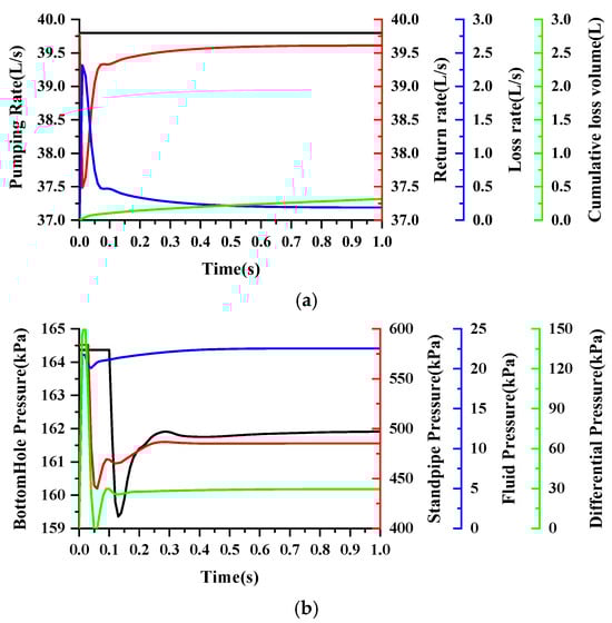
Figure 5.
Parameter variation curves during drilling fluid loss (0~1 s): (a) pumping rate, return flow rate, loss rate, and cumulative loss volume; (b) BHP, standpipe pressure, fluid pressure in fracture, and differential pressure between inlet and outlet.
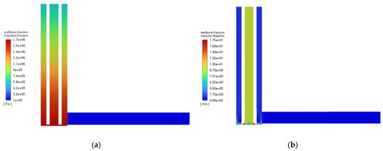
Figure 6.
Cloud map within the coupled wellbore–fracture system (t = 0 s): (a) pressure map; (b) velocity map.
Second stage—Unstable loss stage of drilling fluid: As shown at t = 0–1 s in Figure 5, the drilling fluid invades the inside of the fracture under the action of overbalanced pressure. Since the fracture outlet is a constant-pressure boundary with zero pressure, the pressure difference at both ends of the fracture is the largest at t = 0 s, and the overbalanced pressure is equal to the BHP at the fracture entrance. At the moment of loss, under the drive of the maximum overbalanced pressure, the flow speed of the drilling fluid invading the fracture is the fastest, and the drilling fluid loss rate rises rapidly from zero to reach the peak, defining the flow rate at the moment of loss as the instantaneous loss rate of drilling fluid. Part of the drilling fluid invading the fracture will cause the annular return flow to decrease, breaking the dynamic balance between the inflow and outflow of drilling fluid, so the drilling site will detect a difference between the inflow and outflow of drilling fluid, the total pool volume of drilling fluid will decrease, and the liquid level will drop. The decrease in annular return flow will cause the flow speed of drilling fluid in the annulus to decrease, and the friction between it and the annulus will decrease, so the BHP and standpipe pressure will decrease linearly with time. As the volume of the drilling fluid invading the fracture increases, the fluid pressure in the fracture gradually increases, thereby reducing the overbalanced pressure at both ends of the fracture. The drilling fluid loss rate gradually decreases as the overbalanced pressure decreases, the annular return flow changes from decreasing to increasing over time, and the curve of cumulative loss of drilling fluid increases steadily. The drilling site can monitor that the difference between the inflow and outflow of drilling fluid gradually decreases, the reduction in the total pool volume of drilling fluid per unit time decreases, and the speed of liquid level drop decreases. With the increase in the annular return flow, the BHP and standpipe pressure also change from an initial rapid decrease to an increase.
Figure 7 shows the pressure and velocity cloud map in the coupled wellbore–fracture system at the moment of loss. The pressure in the drill pipe and annulus does not change significantly, but the fluid pressure in the fracture near the entrance area rises due to the invasion of drilling fluid, and the pressure significantly increases compared with that at t = 0 s (Figure 5a). Under the action of the maximum overbalanced pressure, the drilling fluid quickly invades the fracture (Figure 5b).
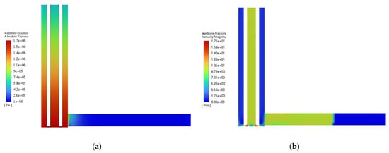
Figure 7.
Cloud map within the coupled wellbore–fracture system (t = 0.1 s): (a) pressure map; (b) velocity map.
Third stage—the stable loss stage of drilling fluid: As shown in Figure 8a, the return flow of drilling fluid in the annulus gradually rises and finally remains constant. In contrast, the curve of loss rate of drilling fluid gradually decreases until it is flat. At this time, there is a constant difference between the return flow in the annulus and the drilling displacement, establishing a new dynamic balance. The curve of the cumulative loss of drilling fluid rises linearly, so the total volume of drilling fluid in the field decreases at a constant rate, and the liquid level decreases uniformly. The pressure response during the loss process corresponds to the changes in flow rate everywhere. Figure 8b shows the changes in various pressures over time during the entire loss process. The pressure curve in the fracture rises slowly and gradually becomes flat. This is due to the decrease in the invasion speed of drilling fluid in the fracture and the increase in the overall loss volume. When the drilling fluid flows out of the constant fracture outlet, the volume of drilling fluid in the fracture does not change, and the pressure in the fracture remains constant. The BHP and standpipe pressure curves also rise and then gradually become flat. This phenomenon indicates that, when the loss rate of drilling fluid is constant, the return flow of the drilling fluid in the annulus is stable, the friction between it and the annulus wall is unchanged, and the BHP and standpipe pressure also remain constant. The trend of the overbalanced pressure curve is consistent with the fluid pressure in the fracture and the BHP, so the drilling fluid maintains stable loss under the constant overbalanced pressure. The pressure and velocity in the fracture are much different from the velocity and pressure in the wellbore. Based on the velocity and pressure distribution cloud map of the coupled wellbore–fracture system, it is difficult to observe the trend of velocity and pressure response in the fracture, so the velocity and pressure cloud map in the fracture are taken separately for analysis. Since the fracture outlet is a constant-pressure boundary, the pressure at the fracture entrance is greater than the pressure at the outlet under the stable loss state, and the pressure gradually decreases along the direction of the fracture length (Figure 9a). As shown in Figure 9b, after the drilling fluid enters the fracture, under the action of flow resistance, the flow rate also gradually decreases along the direction of the fracture length, and is the smallest at the fracture outlet.
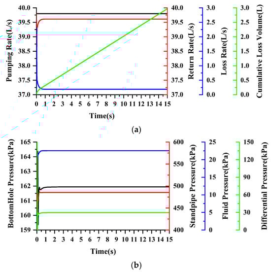
Figure 8.
Parameter variation curves during drilling fluid loss (t = 0~15 s): (a) pumping rate, return flow rate, loss rate, and cumulative loss volume; (b) BHP, standpipe pressure, fluid pressure in fracture, and differential pressure between inlet and outlet.
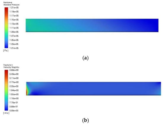
Figure 9.
Cloud map of fracture during drilling fluid loss (t = 15 s): (a) pressure map; (b) velocity map.
3.2. Effect of Overbalanced Pressure
For natural fracture-type loss, the overbalanced pressure of drilling, that is, the difference between the BHP and the formation pressure, often determines the severity of drilling fluid loss. When the formation pressure remains unchanged, the size of the overbalanced pressure mainly depends on the BHP. The BHP during the positive circulation of drilling fluid is mainly affected by the static liquid column pressure in the wellbore and the annular pressure loss. The depth of the well and the density of the drilling fluid determine the size of the static liquid column pressure in the wellbore. The greater the depth of the well and the density of the drilling fluid, the greater the static liquid column pressure in the wellbore. The annular pressure loss is composed of surface manifold pressure loss (pg), inner tool pressure loss (pi), bit pressure loss (pbit), and annulus pressure loss (pa). Due to the simplification of the physical model in the numerical simulation of drilling fluid loss in this paper, the influence of pressure loss in the surface manifold and bit pressure loss on the BHP is ignored, and only the inner pressure loss of the drill pipe and the inner pressure loss of the annulus are considered. The inner pressure loss of the drill pipe and the annulus is mainly determined by the along-path resistance coefficient, drilling fluid density, well depth, drilling fluid flow rate, and the size of the drill pipe and annulus. Among them, the along-path resistance coefficient depends on the properties of the drill pipe and the annulus wall, and is usually taken as a constant. In addition to displacement, viscosity is also an important factor controlling the flow rate of drilling fluid. The Ordos Basin tight sandstone oil and gas reservoir has few drilling openings, and the loss layer is mainly secondary, so the influence of the size of the drill pipe and the annulus on the circulation pressure loss can be ignored. In summary, this work mainly studies the influence of overbalanced pressure on drilling fluid loss by changing the depth of the thief zone, drilling displacement, drilling fluid density, and viscosity.
3.2.1. Well Depth (Location of the Thief Zone)
The depth of the thief zone is one of the important basic parameters for formulating plugging construction measures, which is related to the position of the drill bit and the amount of plugging slurry in the construction. Under the conditions of no loss and stable loss, the BHP–thief zone depth curve is shown in Figure 10a. The BHP almost increases linearly with the depth of the thief zone. This is mainly because the static liquid column pressure is greater than the annular pressure loss. The impact of annular pressure loss brought about by changes in the depth of the thief zone is far less than that of static liquid column pressure, so BHP is nearly linearly related to the well depth. Figure 10b shows the instantaneous loss rate of drilling fluid, stable loss rate, and cumulative loss volume curves. As the depth of the thief zone increases, the curves all show an upward trend, indicating that, as the depth of the thief zone increases, the difference between the inflow and outflow of drilling fluid detected on site is greater, and the total volume of the drilling fluid and the decrease in liquid level height in the same time period are greater. Figure 10c shows that, although the depths of the thief zone are different, under the same fracture geometric conditions, the fluid pressure in the fracture is the same during the stable loss stage, so the greater the BHP corresponding to the stable loss stage, the greater the overbalanced pressure. This explains why the loss rate of drilling fluid increases with the increase in the thief zone depth during the stable loss stage. The loss of drilling fluid will lead to a decrease in standpipe pressure, and the size of the decrease in standpipe pressure reflects the severity of drilling fluid loss. The loss rate of drilling fluid increases with the increase in well depth, and the corresponding decrease in standpipe pressure will also increase with the increase in well depth. The research results of drilling fluid loss behavior at different thief zone depths also explain why, in the drilling process of deep tight oil and gas reservoirs, large loss and severity loss often occur in the lower formations, and the increase in well depth will produce a larger overbalanced pressure.
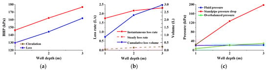
Figure 10.
Drilling fluid loss at different depths of thief zone: (a) BHP; (b) loss rate and cumulative loss volume; (c) different pressures.
3.2.2. Pumping Rate
The size of the drilling displacement will directly affect the flow rate of the drilling fluid in the drill pipe and the annulus, and the size of the flow rate of the drilling fluid determines the annular pressure loss, thereby indirectly affecting the overbalanced pressure. Figure 11a is the BHP–displacement curve during the transition stage of circulation–loss and the stable loss stage. The BHP in both stages increases with the increase in drilling displacement. The increase in drilling fluid displacement will lead to an increase in the flow rate of the drilling fluid in the drill pipe and the annulus, thereby increasing the flow resistance, so the annular pressure loss increases, and the overall BHP increases. As shown in Figure 11b, the instantaneous loss rate and cumulative loss volume curves of drilling fluid show a clear upward trend, and the stable loss rate curve of the drilling fluid is nearly flat, while the response trend of the cumulative loss volume indicates that the stable loss rate curve of drilling fluid also rises with the increase in drilling displacement, but its growth rate is low and the curve slope is small. Comparing the differences in instantaneous and stable loss rates at different drilling displacements, the difference in the inflow and outflow of drilling fluid monitored on site responds within a short time interval. In the stable loss stage, it is difficult to identify the difference between the difference in inflow and outflow, the change in the total volume of drilling fluid, and the change in liquid level height. From Figure 11c, it can also be seen that the slope of the overbalanced pressure and the change value of standpipe pressure is small, and the difference in loss rate at the stable loss stage under different drilling displacements is small, so field drilling often reduces the drilling displacement to measure the loss rate of drilling fluid, while reducing the consumption of drilling fluid and ensuring the accuracy of the measurement of the loss rate of drilling fluid.
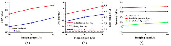
Figure 11.
Drilling fluid loss at different pumping rates: (a) BHP; (b) loss rate and cumulative loss volume; (c) different pressures.
3.2.3. Density of Drilling Fluid
As the well depth increases, it is often necessary to increase the density of the drilling fluid to ensure the stability of the wellbore in the lower formation. However, it often happens that the upper non-loss formation losses after the density of the drilling fluid are increased. This section studies the behavior of drilling fluid loss under different density conditions to clarify the impact of drilling fluid density on loss. The BHP curves in the no loss and stable loss stages both slowly rise with the increase in drilling fluid density, and the overall growth Is small (Figure 12a). From the loss curve, it can be seen that the small difference in BHP leads to a relatively close overbalanced pressure, and the instantaneous loss rate curve of drilling fluid does not change significantly with the increase in drilling fluid density. The stable loss rate curve of the drilling fluid is flat with the change in the drilling fluid density. Only from the increase in cumulative loss volume with the increase in drilling fluid density can it be inferred that the stable loss rate of drilling fluid slowly increases with the increase in drilling fluid density (Figure 12b). Figure 12c also shows that the difference in the stable loss rate of drilling fluid is small, so the difference between the overbalanced pressure is also small, and the change in standpipe pressure is not obvious. The research results show that the slight adjustment of the field drilling density can easily cause the BHP of the upper formation to be greater than the formation pressure and overbalanced pressure occurs, thereby causing the upper non-loss formation to have micro-loss or small loss. However, the response characteristics of this kind of loss are weak, and the minefield is poorly recognizable. Usually, drilling to the lower formation will detect the occurrence of drilling fluid loss, which seriously affects the judgment of the thief zone location.
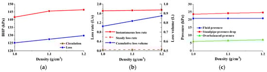
Figure 12.
Drilling fluid loss at different densities of drilling fluid: (a) BHP; (b) loss rate and cumulative loss volume; (c) different pressure.
3.2.4. Viscosity of Drilling Fluid
As can be seen from Figure 13a, unlike well depth, drilling displacement, and drilling fluid density, the change in drilling fluid viscosity has almost no effect on BHP. Figure 13b also shows that the instantaneous loss rate of drilling fluid does not change significantly with the increase in drilling fluid viscosity. A comprehensive analysis of Figure 13b,c found that the stable loss rate and cumulative loss volume curves of the drilling fluid decrease with the increase in drilling fluid viscosity, indicating that the smaller the viscosity of drilling fluid, the greater the stable loss rate of drilling fluid, and the change value of standpipe pressure also confirms this fact. However, the overbalanced pressure curve indicates that, in the stable loss stage, the greater the viscosity of the drilling fluid, the greater its overbalanced pressure. This phenomenon indicates that the increase in drilling fluid viscosity causes an increase in BHP, but the BHP value is far greater than the overbalanced pressure, so, although this difference cannot be reflected in the high order of magnitude of BHP, it is amplified in the low order of magnitude of overbalanced pressure. A smaller overbalanced pressure leads to a larger loss rate of drilling fluid, mainly because the low-viscosity drilling fluid has smaller flow resistance in the same fracture. This research result shows that the high temperature at the bottom of the well during drilling will cause changes in the performance of drilling fluid, such as the reduction in drilling fluid viscosity. In the case of encountering fractures, the loss response characteristics are not obvious, and the loss cannot be identified in time, which causes misjudgment of the thief zone. And the low-viscosity drilling fluid will invade the fracture in large quantities and quickly. Compared with the micro-loss and small loss induced by the change in drilling fluid density, it is very likely to induce more serious loss. Therefore, it is necessary to maintain the performance of drilling fluid in time during drilling, and while ensuring the good wellbore cleaning ability of drilling fluid, it also reduces the probability of serious drilling fluid loss.
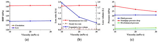
Figure 13.
Drilling fluid loss at different drilling fluid viscosity: (a) BHP: (b) loss rate and cumulative loss volume; (c) different pressures.
As can be seen from the above analysis, changes in the depth of the thief zone, drilling displacement, drilling fluid density, and viscosity will all cause different degrees of drilling fluid loss, as shown in Figure 14. From the size of the values and the slope of the curve, it can be seen that the change in the depth of the thief zone has the greatest impact on the overbalanced pressure, followed by the density of the drilling fluid, and the drilling displacement has the lowest impact on the overbalanced pressure. Under the same fracture geometric parameters, the size of the overbalanced pressure determines the instantaneous loss rate of the drilling fluid, so the response degree of the instantaneous loss rate of the drilling fluid to the four parameters is consistent with the BHP. Different from the instantaneous loss rate of drilling fluid, the depth of the thief zone and the viscosity of drilling fluid have the greatest impact on the stable loss rate of drilling fluid, while the drilling displacement and drilling fluid density have relatively weak effects on it. Excavating the strong and weak quantitative relationship between different variables and the degree of drilling fluid loss helps to understand the microscopic mechanism of drilling fluid loss. Based on the Spearman correlation coefficient method, the results show that the instantaneous loss rate of drilling fluid is strongly positively correlated with the thief zone location and drilling displacement, with a correlation coefficient of 0.73 (Figure 15). The stable loss rate of drilling fluid is strongly positively correlated with the thief zone location and drilling fluid viscosity, and the correlation coefficient is also 0.73. Based on the mathematical model, numerical simulation, and indoor experiments to explore the behavior of drilling fluid loss, a statistical or empirical relationship between the response characteristics of engineering parameters and loss can be established, and thus a drilling fluid loss diagnosis model can be constructed. When establishing a drilling fluid loss diagnosis model, the well depth, drilling displacement, drilling fluid density, viscosity, etc., are used as model input parameters. There are many types, and the correlation with drilling fluid loss is different. Directly using all parameters as model inputs will invisibly increase the redundancy of the model and reduce the efficiency of model operation. Therefore, through quantitative correlation analysis, parameters with a higher correlation with the degree of drilling fluid loss are screened out to achieve the goal of improving the accuracy of drilling fluid loss diagnosis and reducing data redundancy.
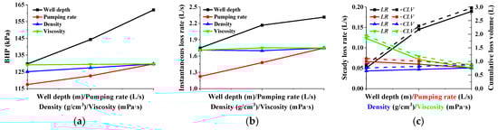
Figure 14.
Effects of depth of thief zone, pumping rate, and drilling fluid properties on drilling fluid loss: (a) BHP; (b) instantaneous loss rate; (c) steady loss rate and cumulative loss volume.
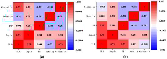
Figure 15.
Results of correlation analysis between level and drilling construction parameters: (a) steady loss rate; (b) instantaneous loss rate.
3.3. Fracture Geometric Parameters
Width, height, length, and geometric shape are important geometric parameters of fractures. The size of fracture geometric parameters often determines the along-path resistance coefficient of drilling fluid loss channels, the size of loss channels, and the limit accommodation space, thereby affecting the loss behavior of drilling fluid in fractures. This section discusses the impacts of width, height, length, and geometric shape on the behavior of drilling fluid loss through the TFM drilling fluid loss model.
3.3.1. Fracture Width
As shown in Figure 16a, the instantaneous loss rate of drilling fluid increases nearly linearly with the increase in fracture width, while the stable loss rate of drilling fluid and the cumulative loss of drilling fluid increase non-linearly with the increase in fracture width. The larger the loss fracture width, the more severe the drilling fluid loss caused by it, so the difference between the drilling fluid inflow and outflow detected on site is also larger, and the total volume and liquid level of the drilling fluid pool drop more. The higher the severity of drilling fluid loss, the smaller the return flow rate of drilling fluid in the annulus, which means that the BHP corresponding to the stable loss stage is smaller. As can be seen from Figure 16b, the BHP at the stable loss stage decreases non-linearly with the increase in loss fracture width. The standpipe pressure is also related to the return flow rate of drilling fluid in the annulus. When the severity of drilling fluid loss is higher, the decrease in return flow rate compared with the dynamic balance during circulation is greater, and the corresponding decrease in standpipe pressure detected is greater (Figure 16c). Therefore, when the construction parameters are similar, the relative geometric size of the loss fracture can be preliminarily determined through the response trend of the engineering parameters during the loss process. The fluid pressure in the fracture during the stable loss stage increases linearly with the increase in fracture width. This is mainly because, when the fracture height and length remain unchanged, the volume in the fracture is determined by the fracture width. Therefore, when the fracture width increases, the volume in the fracture increases and keeps consistent with the growth trend of the width. The volume in the fracture determines the size of the fluid pressure in the fracture. Contrary to the trend of stable loss rate, the pressure difference at both ends of the fracture during the stable loss stage will decrease with the increase in fracture width. The larger the fracture width, the more severe the drilling fluid loss caused by it, the greater the fluid pressure in the fracture, and the smaller the BHP corresponding to the stable loss stage, so the corresponding overbalanced pressure is also smaller. The wider the fracture, the greater the loss rate under a smaller overbalanced pressure than that of a narrower fracture under a larger overbalanced pressure. The loss rate of drilling fluid is the volume of drilling fluid flowing over the cross-section of the loss fracture per unit time, so the loss rate of the drilling fluid is a function of the size of the cross-sectional area of the fracture entrance and the flow velocity of drilling fluid. This section will study the response characteristics of the entrance flow rate to pressure for loss fractures of different widths through the analysis of the entrance flow velocity. Figure 16d shows the flow velocity at the entrance of the fracture with different drilling fluid instantaneous loss rates and stable loss rates. In the unstable loss stage, under the same overbalanced pressure, the instantaneous flow velocity of drilling fluid through the fracture entrance does not show a significant upward trend with the increase in fracture width, and the difference in flow velocity is small. However, the flow velocity of the drilling fluid through the fracture entrance during the stable loss stage will show a significant upward trend with the increase in fracture width, and the difference in flow velocity will be significant. Relative to the wellbore radius, the fracture entrance is a necked narrow mouth, so when the drilling fluid returning along the annulus is diverted at the fracture entrance, it is similar to the free submerged outflow in the pipeline, and a local water head loss will occur at the fracture entrance. The larger the fracture width, the smaller the corresponding equivalent hydraulic radius, and the smaller the local loss coefficient. The small difference in instantaneous flow velocity at the entrance of fractures of different widths indicates that the response trend of local water head loss to pressure difference is different. Under a larger pressure difference, the change in width from 1 to 5 mm has little effect on local water head loss, so the flow velocity of the drilling fluid at the entrance of fractures with a width of 1 to 5 mm in the unstable loss stage is small, and the difference in instantaneous loss rate of drilling fluid is mainly caused by the size of the cross-sectional area of the fracture entrance. However, as the overbalanced pressure in the stable loss stage decreases, the response degree of local water head loss becomes stronger. A wider fracture has a smaller local loss coefficient, so even though its overbalanced pressure is smaller, the flow velocity at the fracture entrance is actually larger. Therefore, in deep formations, the overbalanced pressure increases with the increase in well depth. Under the action of a larger order of magnitude pressure, the loss rate of drilling fluid more reflects the difference between the geometric features of the loss fracture. Based on the response characteristics of engineering parameters, it is more advantageous to diagnose the geometric size of the loss fracture.
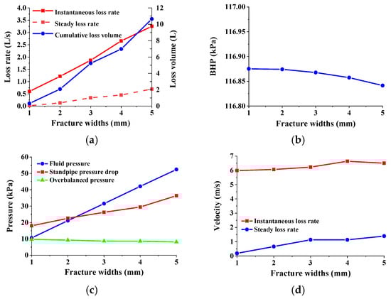
Figure 16.
Drilling fluid loss at different fracture widths: (a) loss rate and cumulative loss volume; (b) BHP; (c) different pressure; (d) flow velocity at fracture inlet.
3.3.2. Fracture Height
Figure 17a shows that the instantaneous loss rate, stable loss rate, and cumulative loss volume of drilling fluid all linearly increase with the increase in fracture height. Larger fractures will lead to more severe drilling fluid loss, and the larger the drilling fluid loss rate in the stable loss stage, the smaller the BHP (Figure 17b). The fluid pressure in the fracture will increase with the increase in the volume of the fracture, so for fractures with larger fracture heights, the BHP in the stable loss stage is smaller, the fluid pressure in the fracture is larger, and the corresponding overbalanced pressure is smaller (Figure 17c). The decrease in standpipe pressure increases with the increase in fracture height, which is due to the more severe drilling fluid loss caused by higher fractures, the smaller the annular return flow rate, and therefore the smaller the flow friction between the drilling fluid and the annulus. Figure 17d shows that the flow velocity of the drilling fluid at the entrance of the fracture during the unstable loss stage tends to decrease with the increase in height. This is because, as the fracture height increases, the well depth corresponding to the upper part of the higher fracture is smaller, the corresponding overbalanced pressure is smaller, and the average flow velocity on the cross section of the fracture entrance is smaller under the same fracture width. In the stable loss stage, the overbalanced pressure decreases with the increase in fracture height, so the flow velocity at the fracture entrance also shows a downward trend with the increase in fracture height.
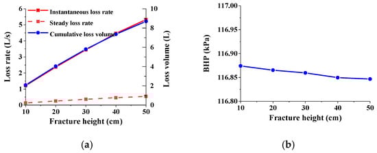
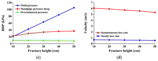
Figure 17.
Drilling fluid loss at different fracture height: (a) loss rate and cumulative loss volume; (b) BHP; (c) different pressure; (d) flow velocity at fracture inlet.
3.3.3. Fracture Length
As shown in Figure 18a, the loss rate and cumulative loss volume of drilling fluid under different fracture lengths. The instantaneous loss rate of drilling fluid is a straight line segment with the increase in fracture length, and the flow rate at the fracture entrance is equal under the same overbalanced pressure, fracture width, and fracture height. The curve of the stable loss rate and cumulative loss volume of drilling fluid decreases with the increase in fracture length, and the slope gradually decreases. It is difficult to identify the length of the loss fracture based on the difference between the inflow and outflow of drilling fluid. When the fracture is long enough, there is basically no difference in the total pool volume and liquid level height of the drilling fluid. In the stable loss stage, the BHP curve first rises and then gradually approaches a straight line with the increase in fracture length. The reason why the instantaneous loss rate of drilling fluid is equal and the stable loss rate is different is that the volume in the fracture increases with the increase in fracture length, so the fluid pressure in the fracture increases with the increase in fracture length (Figure 18c). When the BHP is close, the larger the fluid pressure in the fracture, the smaller the corresponding overbalanced pressure, so the loss rate of drilling fluid in the stable loss stage is smaller. The size of the decrease in standpipe pressure indicates the severity of drilling fluid loss, so from the trend of standpipe pressure change, it can also be seen that the longer the fracture length, the weaker the drilling fluid loss. Under the same pressure difference, fracture width, and fracture height, the instantaneous flow velocity at the fracture entrance is equal, and the flow velocity at the entrance during the stable loss stage is consistent with the loss rate of drilling fluid. Due to the smaller loss pressure difference, the flow velocity at the fracture entrance decreases with the increase in fracture length.
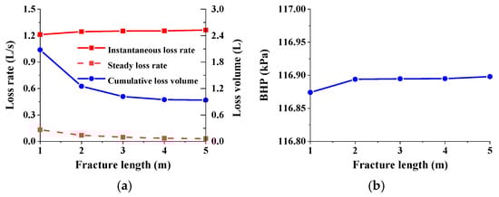
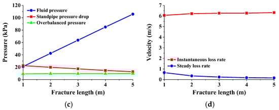
Figure 18.
Drilling fluid loss at different fracture lengths: (a) loss rate and cumulative loss volume; (b) BHP; (c) different pressures; (d) flow velocity at fracture inlet.
In Figure 19, the relationship between the loss rate and time of fractures with different widths, heights, and lengths is shown. As mentioned earlier, the overbalanced pressure is the largest at the moment when the drilling fluid loss occurs, so in all simulation results, the instantaneous loss rate of drilling fluid is reached at the first time step (i.e., t = 0.01 s). As the loss time of drilling fluid extends, the overbalanced pressure decreases with the increase in fluid pressure in the fracture, and the loss rate of drilling fluid decreases accordingly. When the fluid pressure in the fracture remains unchanged, the pressure difference at both ends of the fracture will remain constant, and the loss rate of drilling fluid will stabilize. Based on the loss curve, it can be found that the time required for fractures with different geometric parameters to reach stable loss is different, and the time required for fractures with different geometric parameters to reach stable loss is shown in Figure 20. In this paper, the time required to reach stable loss is equal to the time required for drilling fluid to invade to the fracture outlet, so this time reflects the speed of drilling fluid invasion in the fracture. The time required to reach stable loss shortens with the increase in fracture width. Although the flow velocity at the fracture entrance is basically the same as that in the instantaneous loss stage, the flow velocity at the entrance of the wider fracture is larger with the extension of loss time, and its along-course resistance coefficient is smaller, so the invasion depth in the fracture is deeper within the same time. For fracture height, the change in fracture height has no obvious effect on the time required to reach stable loss, and the time required to reach stable loss is basically the same. However, the time required to reach stable loss will first increase rapidly and then tend to be stable with the increase in fracture length, mainly because the increase in fracture length increases the invasion depth required for drilling fluid in the fracture, so the time required to reach stable loss is relatively longer. Based on field logging engineering data, the time required for field drilling fluid from loss occurrence to stable loss can be read from the change curve of the difference between drilling fluid inflow and outflow with time, so by comparing the loss under different conditions, the relative geometric characteristics of drilling fluid loss channel can be preliminarily judged.
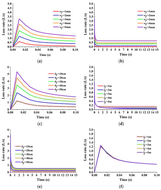
Figure 19.
Curve of drilling fluid loss rate with time for different fracture geometric characteristics: (a) 0–0.1 s drilling fluid loss rate at different fracture widths; (b) 0–15 s drilling fluid loss rate at different fracture widths; (c) 0–0.1 s drilling fluid loss rate at different fracture heights; (d) 0–15 s drilling fluid loss rate at different fracture heights; (e) 0–0.1 s drilling fluid loss rate at different fracture lengths; (f) 0–15 s drilling fluid loss rate at different fracture lengths.
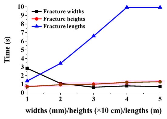
Figure 20.
Time required to achieve stable loss under different fracture geometric characteristics.
3.4. Fracture Geometry
The natural fractures encountered in the actual drilling process are not parallel fractures with a uniform width along the length of the fracture. During the loss process, when the fluid pressure in the fracture is greater than the stress intensity factor at the fracture tip, the fracture will extend forward. The fluid pressure in the fracture will also overcome the normal stress on the fracture wall surface, resulting in an increase in the width of the fracture. As shown in Figure 21, when the fracture stops spreading, it is in the shape of a wedge with a wide fracture entrance and a narrow front end. This section focuses on investigating how geometric parameters of wedge-shaped fractures affect drilling fluid loss.
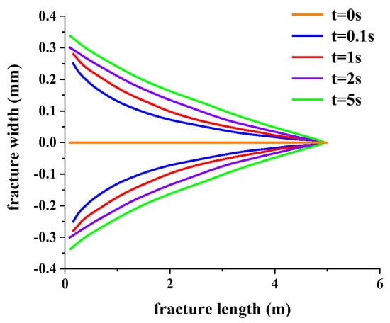
Figure 21.
Characteristics of fracture morphological changes during loss.
3.4.1. Wedge Fractures with Varying Outlet Width
For fractures of equal height and length, the influence of wedge-shaped fractures with different inlet/outlet width ratios on the loss behavior of drilling fluid is explored by keeping the fracture inlet width constant and changing the fracture outlet width. As shown in Figure 22, the numerical simulation results of drilling fluid loss in wedge-shaped fractures with an inlet width of 5 mm and outlet widths of 1–5 mm are presented. Under the same overbalanced pressure, the instantaneous loss rate of drilling fluid in fractures with different outlet widths is basically the same, and the curve is a straight-line segment. The stable loss rate and cumulative loss of drilling fluid increase with the increase in the outlet width of the wedge-shaped fracture, and the slope of the curve gradually decreases (Figure 22a). The difference between the inflow and outflow of drilling fluid and the total volume change of the drilling fluid (change in liquid level height) are common methods to identify drilling fluid loss. Comparing the engineering logging data when different losses occur, it is found that, when the initial difference between the inflow and outflow of drilling fluid is equal and then gradually differentiated, the wedge-shaped fracture with equal inlet width and unequal outlet width may be one of the causes of this phenomenon. Consistent with the trend of BHP changes, the change in standpipe pressure reflecting the severity of loss increases with the increase in outlet fracture width (Figure 22b,c). In the stable loss stage, the increase in fracture outlet width leads to an increase in fracture volume, so the fluid pressure in the fracture increases with the increase in fracture outlet width. For fractures with larger outlet widths, the BHP in the stable loss stage is smaller and the fluid pressure in the fracture is larger, so the corresponding overbalanced pressure is smaller. From Figure 22d, we can see that, for wedge-shaped fractures with unequal inlet widths and equal outlet widths, the trend of drilling fluid velocity at the inlet at different stages with width is consistent with that of parallel fractures with different fractures widths. Under the same pressure difference, the inlet velocity of fractures with the same inlet width is basically the same, and the corresponding instantaneous loss rate is also basically the same. However, the larger the outlet width, the smaller the flow resistance of drilling fluid in the fracture, so even under a smaller positive pressure difference, the loss rate of drilling fluid in the fracture with a wider outlet is larger. Unlike parallel fractures, for wedge-shaped fractures with equal inlet width and equal outlet width, the main stable loss rate is the flow difference caused by the difference in inlet flow velocity.
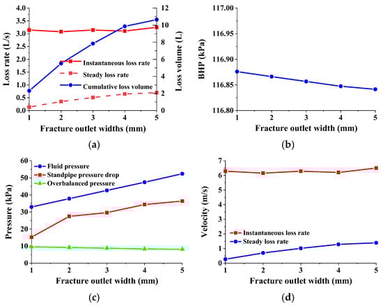
Figure 22.
Drilling fluid loss of wedge-shaped fractures with different outlet width: (a) loss rate and cumulative loss volume; (b) BHP; (c) different pressures; (d) flow velocity at fracture inlet affecting drilling fluid loss.
3.4.2. Wedge Fractures with Varying Inlet Width
After discussing the behavior of drilling fluid loss in wedge-shaped fractures with equal inlet widths and unequal outlet widths, the numerical simulation results of drilling fluid loss in wedge-shaped fractures with different inlet widths and equal outlet widths are shown in Figure 23. As shown in Figure 23a, the instantaneous loss rate and cumulative loss curve of drilling fluid increase linearly with the increase in inlet width, while the trend of cumulative loss curve indicates that the stable loss rate of drilling fluid also increases with the increase in inlet fracture width. The BHP and standpipe pressure drop value decrease overall with the increase in the inlet width of the wedge-shaped fracture, but the difference in loss rate between different inlet width wedge-shaped fractures is small, and the difference between the BHP and standpipe pressure drop value is not significant (Figure 23b,c). The fluid pressure in the fracture mainly depends on the size of the volume in the fracture. The fluid pressure in the fracture increases with the increase in the opening of the wedge-shaped fracture inlet, while the overbalanced pressure decreases with the increase in the inlet width of the wedge-shaped fracture. Figure 23d also shows that, for fractures with different inlet widths, when the overbalanced pressure is large, the drilling fluid flow velocity is less affected by the local resistance coefficient, and the instantaneous flow velocity of the drilling fluid at the fracture inlet is basically equal when loss occurs. With the extension of drilling fluid loss time, the rapid growth of fluid pressure in the fracture will lead to a decrease in overbalanced pressure. Under the condition of low overbalanced pressure, the flow velocity of drilling fluid at the fracture inlet is greatly affected by the local resistance coefficient. However, the smaller the fracture inlet width, the larger the corresponding overbalanced pressure, so the flow velocity of drilling fluid at the inlet of wedge-shaped fractures with different inlet widths is basically equal during the stable loss stage. For wedge-shaped fractures with different inlet widths and the same outlet width, the difference between the instantaneous loss rate and the stable loss rate of drilling fluid is caused by the size of the cross-section at the fracture inlet.
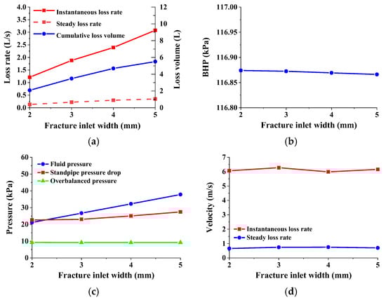
Figure 23.
Drilling fluid loss of wedge-shaped fractures with different inlet width: (a) loss rate and cumulative loss volume; (b) BHP; (c) different pressure; (d) flow velocity at fracture inlet.
From the above study, it can be found that, although the geometric shape, width, height, and length of the fracture directly affect the behavior of drilling fluid loss and determine the severity of drilling fluid loss, the response characteristics and trends of drilling fluid loss severity to different parameters are different. As shown in Figure 24a, the horizontal axis direction is the direction of increasing fracture geometric parameters. It can be seen that the instantaneous loss rate of drilling fluid mainly depends on the size of the cross-section at the fracture inlet. When the cross-sectional size is equal (when the width and height of the fracture are equal), the instantaneous loss rate of drilling fluid is equal. The instantaneous loss rate of drilling fluid will increase with the increase in the cross-sectional area of the fracture inlet, and the increase in fracture height has a greater impact on the instantaneous loss rate than the fracture width. For parallel fractures and wedge-shaped fractures, it can also be found that the instantaneous loss rate of drilling fluid is independent of the size of the cross-section at the fracture outlet. As shown in Figure 24b,c, with the change in fracture geometry and geometric parameters, the stable loss rate and cumulative loss of drilling fluid have the same response trend. The response trend of the drilling fluid stable loss rate (cumulative loss) to fracture geometry and geometric parameters is more complex. The ratio of the inlet width to the outlet width of the wedge-shaped fracture is defined as Rw. Due to the uniform necking of the wedge-shaped fracture along the fracture length direction, the geometry of the wedge-shaped fracture can be characterized by Rw and fracture length. The correlation coefficient of the drilling fluid stable loss rate with fracture geometry and parameters is shown in Figure 25. The stable loss rate of drilling fluid is positively correlated with the inlet width of the fracture, Rw, and fracture height. Among them, the correlation with the inlet width of the fracture is the highest, and the correlation between the geometry of the fracture and the stable loss rate of drilling fluid is poor. The fracture length is strongly negatively correlated with the stable loss rate of drilling fluid, with a correlation coefficient of −0.62.
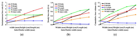
Figure 24.
Effect of fracture geometric characteristic parameters on drilling fluid: (a) instantaneous loss rate; (b) steady loss rate; (c) cumulative loss volume.
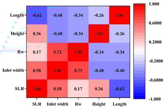
Figure 25.
Correlation coefficient between drilling stable loss rate and fracture geometric parameters.
Comparing the time required for parallel fractures and wedge fractures to reach stable loss, it is found that there is a diameter expansion at the entrance of the wedge fracture relative to the exit. The existence of the expansion effect causes the instantaneous flow rate at the entrance of the wedge fracture to be larger, and the smaller the resistance coefficient, the shorter the time required for the wedge fracture to reach stable loss for the same exit width as the parallel fracture (Figure 26). When the width of the entrance of the wedge fracture is certain, the width of the exit has no significant effect on the time required to reach stable loss.
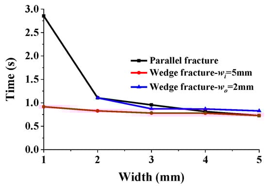
Figure 26.
Time required for parallel fracture and wedge fracture of different widths to reach stable loss.
4. Fields Application
The working environment of drilling construction is hidden underground, and the process status of the operation is usually understood through a brief introduction of surface drilling parameters, which involves a lot of fuzziness, randomness, and uncertainty. Among them, drilling fluid loss is one of the most common complex situations in the well. Timely, efficient, and accurate diagnosis of drilling fluid loss is of great significance for the safety and economy of drilling operations. Key information, such as the location of the thief zone, the type of loss, and the size of the loss channel is obtained through the diagnosis of drilling fluid loss, thereby providing support for the control of drilling fluid loss. Common methods for diagnosing drilling fluid loss mainly include the chart method (empirical curve method) and the comprehensive logging method. The chart method first solves the classic drilling fluid loss model under different fracture geometries, and initial and boundary conditions, obtains a series of drilling fluid loss rate (cumulative loss volume)–time relationship curves, and then compares the field drilling fluid loss data with the formed series. The curve is fitted to diagnose the width of the loss fracture. The key information obtained by the chart method is only the geometric size of the loss fracture, and the diagnosed information is relatively one-sided. The mathematical model of drilling fluid loss is usually simplified, and the working condition it simulates is far from the real loss condition, so the diagnosed information has a huge deviation.
Any complex situation in the well will produce signs in the parameter records of the drilling instrument, often manifested in different forms of changes in different engineering parameters. The comprehensive logging method is the most widely used method for diagnosing drilling fluid loss. It monitors logging parameters in real time, such as standpipe pressure, drilling time, torque, hook load, hook height, inlet and outlet flow, total pool volume, etc., and analyzes the abnormal changes in these characteristic parameters to find their rules and achieve the diagnosis of drilling fluid loss. Among them, the change value of the standpipe pressure, the difference in drilling fluid inlet and outlet flow, and the change value of the total drilling fluid pool volume are the most commonly used engineering parameters for diagnosing drilling fluid loss. As shown in Figure 27, a larger difference in drilling fluid inlet and outlet flow (instantaneous drilling fluid loss rate) does not mean that the change in total drilling fluid pool volume (cumulative drilling fluid loss) is larger. An increase in fracture length or an increase in drilling fluid viscosity will lead to a weakening of the subsequent loss severity. Even if the difference in the drilling fluid inlet and outlet flow (change in total drilling fluid pool volume) is equal, the change in standpipe pressure may not necessarily be equal. This is because the performance parameters of drilling fluid (such as density and viscosity), drilling displacement, thief zone location, fracture geometric parameters (fracture width, fracture height, fracture length, and fracture morphology) jointly determine the severity of drilling fluid loss, and the severity of drilling fluid loss is reflected in the drilling fluid inlet and outlet flow difference, drilling fluid total pool volume change, and standpipe pressure change value. The depth of the thief zone and the width of the fracture are the most important parameters for field plugging construction. Figure 28 shows the scatter plot of engineering response characteristics when fractures of different depths and widths occur. The size of the scatter point represents the relative depth of the thief zone. The larger the scatter point, the deeper the thief zone. The depth of the scatter point color represents the relative size of the fracture width. The darker the scatter point color, the smaller the fracture width. However, the changes in different engineering parameters have different responses to each variable. A change in a single variable may cause the engineering parameters to change together, or it may cause any one or two of them to change. Therefore, compared with the chart method, the comprehensive logging method is more accurate in diagnosing drilling fluid loss, and it is easier to identify the detailed changes in the response of engineering parameters brought about by different factors.
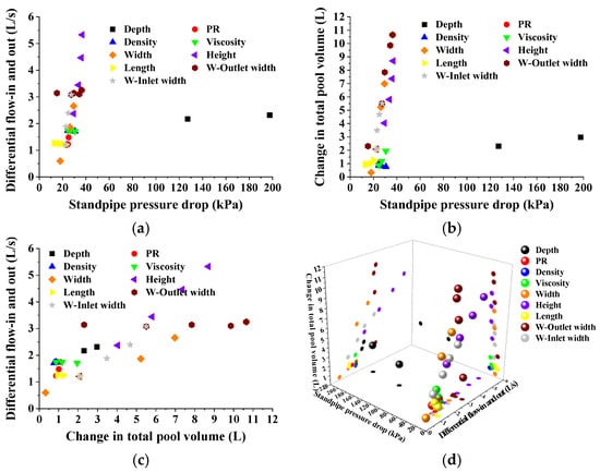
Figure 27.
Scatter diagrams of response characteristics of engineering parameters and related influencing factors: (a) Differential flow-in and out—standpipe pressure drop; (b) Change in total pool volume—standpipe pressure drop; (c) Differential flow-in and out—Change in total pool volume; (d) 3D scatter diagram.
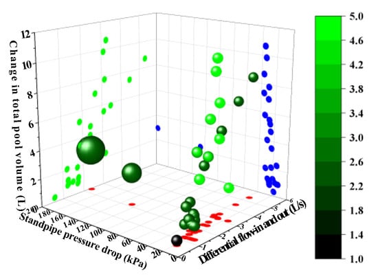
Figure 28.
3D scatter map of the diagnosis of thief zone location and loss fracture width based on the response characteristics of engineering parameters.
The comprehensive logging method requires a large number of loss data samples, and the recognition accuracy of field monitoring instruments for changes in engineering parameters may also cause problems such as wellbore information lag and untimely diagnosis. The rapid development of large-scale simulation technology and the proposal of artificial intelligence technology provide a new idea for drilling fluid loss diagnosis: carrying out drilling fluid loss behavior simulation based on a wellbore-fracture coupling system with high reproducibility, and changing the wellbore size, drilling tool combination, drilling displacement, drilling fluid performance parameters, thief zone depth, and fracture geometric characteristics parameters to obtain a large amount of drilling fluid loss data and corresponding engineering response characteristics that have a high degree of fit with the real loss situation. Figure 29 illustrates the variations in logging parameters during a lost circulation incident in an appraisal well within a Sichuan Basin carbonate gas reservoir. At the onset of lost circulation, a reduction in the outflow rate of drilling fluid was first observed. While the inflow rate remained constant, the inflow–outflow flow rate differential (i.e., drilling fluid loss rate) increased significantly from zero. Concurrently, standpipe pressure exhibited an instantaneous drop, and the total pit volume began to decrease. As lost circulation progressed, the field-measured inflow–outflow differential stabilized, the total pit volume decreased linearly, and the stabilized standpipe pressure, due to reduced outflow, remained lower than the pre-loss baseline. A comparison with Figure 28 demonstrates that the simulated loss data closely matched the field logging parameters, with the most pronounced responses observed in the total pit volume variation, inflow–outflow flow rate differential, and standpipe pressure change. The drilling fluid loss data and corresponding engineering response characteristics obtained from the field and simulation are further learned through artificial intelligence technology to establish a corresponding drilling fluid loss diagnosis case library. Finally, on the basis of improving the monitoring accuracy of field engineering data changes, the drilling fluid loss diagnosis case library is connected to the drilling real-time system to achieve timely discovery, early warning, and diagnosis of drilling fluid loss (Figure 30).
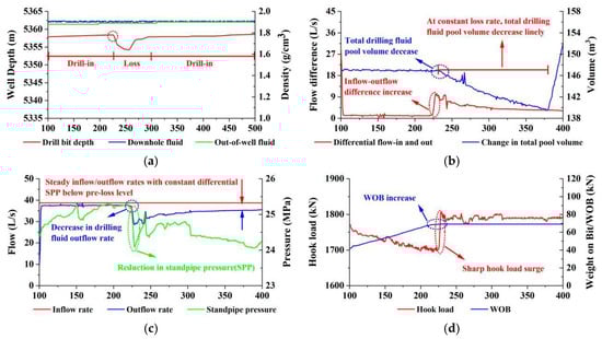
Figure 29.
Lost circulation logging parameters of Well DT1 in Sichuan Basin carbonate gas reservoirs: (a) Bit position, and inflow and outflow drilling fluid density; (b) Inflow/outflow differential and total mud pit volume variation; (c) Inflow rate, outflow rate, and standpipe; (d) Hook load and weight on bit.
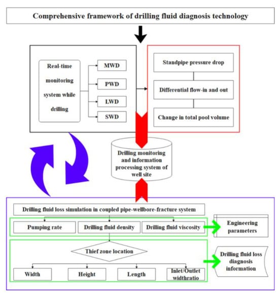
Figure 30.
Schematic diagram of comprehensive framework of drilling fluid diagnosis technology.
5. Conclusions
The drilling fluid loss problem in natural fractured formations was studied using a two-phase model that integrated drilling construction parameters, drilling fluid rheological properties, and fracture geometry parameters. The present model was compared with the previous literature and experiments, and good agreement was obtained. Summarizing the simulation results, the following conclusions were drawn:
- (1)
- A two-phase flow model for drilling fluid within the wellbore–fracture system was established based on the Eulerian–Eulerian approach, incorporating dynamic BHP and solid-phase distribution effects into the loss process simulation. Validated against literature data and experimental results with an average error ≤ 8%, the model demonstrates precise characterization of transient lost circulation behavior in deep fractured formations, overcoming the limitation of conventional single-phase models in underestimating loss severity.
- (2)
- Dynamic BHP is the primary controlling factor of drilling fluid loss behavior. During drilling circulation, annular fractional pressure losses significantly elevate BHP, consequently exacerbating fluid loss. Well depth exerts a near-linear growth effect on BHP, followed by pumping rate, whereas adjustments in drilling fluid density and viscosity exhibit a minimal impact on BHP. Quantitative analysis reveals that well depth shows a strong correlation with instantaneous loss rate (Spearman’s ρ = 0.73), and viscosity correlates strongly with steady loss rate (correlation coefficient = 0.73).
- (3)
- Fracture geometric parameters exert differential control on drilling fluid loss behavior. Fracture width has a significantly stronger impact on loss rate than height. A width increase of 1–5 mm induces linear growth in the instantaneous loss rate and a non-linear enhancement in steady loss rate. An increase in fracture height reduces the average flow velocity within the fracture. Fracture elongation elevates fluid pressure along the fracture, leading to a reduced driving pressure differential, thereby decreasing the steady loss rate. For wedge-shaped fracture (wider entrance/narrow exit), the entrance-widening effect shortens the time to reach steady loss by 20–40%, intensifying initial losses.
- (4)
- A multi-parameter response-based prediction–diagnosis framework for lost circulation is proposed: ① Instantaneous loss rate reflects the cross-sectional area at the fracture entrance; ② Steady loss rate is synergistically controlled by fracture width, well depth, and fluid viscosity; ③ Standpipe pressure drop combined with total pit volume variation jointly indicates geometric dimensions of loss channels (responsiveness hierarchy: width > height > length); ④ An AI-powered “simulation-monitoring” intelligent diagnostic knowledge base enables real-time identification of loss zone depth and fracture width (error < 10%), guiding optimization of lost circulation material (LCM) strategies.
Author Contributions
Conceptualization, Y.K.; Investigation, Z.X.; Methodology, Z.X.; Supervision, Y.K.; Validation, C.X.; Visualization, X.W.; Writing-original draft, Z.X.; Writing-review and editing, C.L. All authors have read and agreed to the published version of the manuscript.
Funding
This research was funded by the Science and Technology Project of PetroChina Southwest Oil & Gasfield Company (No. 25XNYTSC008).
Data Availability Statement
The original contributions presented in this study are included in the article. Further inquiries can be directed to the corresponding author.
Acknowledgments
The authors gratefully acknowledge the financial support from the Science and Technology Project of PetroChina Southwest Oil & Gasfield Company (No. 25XNYTSC008).
Conflicts of Interest
Authors Zhichao Xie and Xueqiang Wang were employed by the Engineering Technology Research Institute of Southwest Oil & Gas Field Company. Author Chong Lin was employed by CCDC Drilling & Production Technology Research Institute. The authors declare that this study received funding from the Science and Technology Project of PetroChina Southwest Oil & Gasfield Company. The funder was not involved in the study design, collection, analysis, interpretation of data, the writing of this article, or the decision to submit it for publication.
References
- Kang, Y.; Xu, C.; You, L.; Yu, H.; Zhang, B. Comprehensive evaluation of formation damage induced by working fluid loss in fractured tight gas reservoir. J. Nat. Gas Sci. Eng. 2014, 18, 353–359. [Google Scholar] [CrossRef]
- Ozdemirtas, M.; Kuru, E.; Babadagli, T. Experimental investigation of borehole ballooning due to flow of non-Newtonian fluids into fractured rocks. Int. J. Rock Mech. Min. Sci. 2010, 47, 1200–1206. [Google Scholar] [CrossRef]
- Gharbi, S.; Al Majed, A.A.; Abdulraheem, A.; Patil, S.; Elkatatny, S. What is the best artificial intelligent technology to solve drilling challenges? In Proceedings of the SPE Conference at Oman Petroleum and Energy Show, Muscat, Oman, 21–23 March 2022. [Google Scholar]
- Gunawan, A.Y.; Sukarno, P.; Soewono, E. Modelling of formation damage due to mud filtrate invasion in a radial flow system. J. Pet. Sci. Eng. 2012, 100, 99–105. [Google Scholar]
- Mirzaei-Paiaman, A.; Masihi, M.; Moghadasi, J. Formation damage through aqueous phase trapping: A review of the evaluating methods. Pet. Sci. Technol. 2011, 29, 1187–1196. [Google Scholar] [CrossRef]
- Civan, F. Reservoir Formation Damage; Gulf Professional Publishing: London, UK, 2015. [Google Scholar]
- Bennion, D.B. An overview of formation damage mechanisms causing a reduction in the productivity and injectivity of oil and gas producing formations. J. Can. Pet. Technol. 2002, 41, 29–36. [Google Scholar] [CrossRef]
- Krishna, S.; Ridha, S.; Vasant, P.; Ilyas, S.U.; Sophian, A. Conventional and intelligent models for detection and prediction of fluid loss events during drilling operations: A comprehensive review. J. Pet. Sci. Eng. 2020, 195, 107818. [Google Scholar] [CrossRef]
- Murtaza, M.; Tariq, Z.; Zhou, X.; Al-Shehri, D.; Mahmoud, M.; Kamal, M.S. Okra as an environment-friendly fluid loss control additive for drilling fluids: Experimental & modeling studies. J. Pet. Sci. Eng. 2021, 204, 108743. [Google Scholar]
- Lavrov, A. Modeling flow of a biviscous fluid from borehole into rock fracture. J. Appl. Mech. 2006, 73, 171–173. [Google Scholar] [CrossRef]
- Bondarenko, A.V.; Islamov, S.R.; Ignatyev, K.V.; Mardashov, D.V. Laboratory studies of polymer compositions for well-kill under increased fracturing. Perm J. Pet. Min. Eng. 2020, 20, 37–48. [Google Scholar] [CrossRef]
- Majidi, R.; Miska, S.Z.; Ahmed, R.; Yu, M.; Thompson, L.G. Radial flow of yield-power-law fluids: Numerical analysis, experimental study and the application for drilling fluid losses in fractured formations. J. Pet. Sci. Eng. 2010, 70, 334–343. [Google Scholar] [CrossRef]
- Majidi, R.; Miska, S.Z.; Yu, M.; Thompson, L.G.; Zhang, J. Quantitative analysis of mud losses in naturally fractured reservoirs: The effect of rheology. SPE Drill. Complet. 2010, 25, 509–517. [Google Scholar] [CrossRef]
- Jia, L.; Chen, M.; Hou, B.; Sun, Z.; Jin, Y. Drilling fluid loss model and loss dynamic behavior in fractured formations. Pet. Explor. Dev. 2014, 41, 105–112. [Google Scholar] [CrossRef]
- Belousov, A.; Lushpeev, V.; Sokolov, A.; Sultanbekov, R.; Tyan, Y.; Ovchinnikov, E.; Shvets, A.; Bushuev, V.; Islamov, S. Experimental Research of the Possibility of Applying the Hartmann–Sprenger Effect to Regulate the Pressure of Natural Gas in Non-Stationary Conditions. Processes 2025, 13, 1189. [Google Scholar] [CrossRef]
- Xia, Y.; Jin, Y.; Chen, M. Comprehensive methodology for detecting fracture aperture in naturally fractured formations using mud loss data. J. Pet. Sci. Eng. 2015, 135, 515–530. [Google Scholar] [CrossRef]
- Feng, Y.; Gray, K.E. Modeling lost circulation through drilling-induced fractures. SPE J. 2018, 23, 205–223. [Google Scholar] [CrossRef]
- Wang, C.; Huang, Z.; Wu, Y. Coupled numerical approach combining X-FEM and the embedded discrete fracture method for the fluid-driven fracture propagation process in porous media. Int. J. Rock Mech. Min. Sci. 2020, 130, 104315. [Google Scholar] [CrossRef]
- Wu, Y.-S.; Lai, B.; Miskimins, J.L.; Fakcharoenphol, P.; Di, Y. Analysis of multiphase non-Darcy flow in porous media. Transp. Porous Media 2011, 88, 205–223. [Google Scholar] [CrossRef]
- Wei, Q.; Zhou, H.; Yang, S. Non-Darcy flow models in porous media via Atangana-Baleanu derivative. Chaos Solitons Fractals 2020, 141, 110335. [Google Scholar] [CrossRef]
- Bannister, C.E.; Lawson, V.M. Role of cement fluid loss in wellbore completion. In Proceedings of the SPE Annual Technical Conference and Exhibition, Las Vegas, NV, USA, 22–26 September 1985. [Google Scholar]
- Bruckdorfer, R.; Gleit, A. Static fluid loss model. SPE Gen. 1988, 20. [Google Scholar]
- Dyke, C.G.; Wu, B.; Milton-Tayler, D. Advances in characterizing natural-fracture permeability from mud-log data. SPE Form. Eval. 1995, 10, 160–166. [Google Scholar] [CrossRef]
- Zimmerman, R.W.; Bodvarsson, G.S. Hydraulic conductivity of rock fractures. Transp. Porous Media 1996, 23, 1–30. [Google Scholar] [CrossRef]
- Lietard, O.; Unwin, T.; Guillot, D.; Hodder, M. Fracture width LWD and drilling mud/LCM selection guidelines in naturally fractured reservoirs. In Proceedings of the European Petroleum Conference, Milan, Italy, 22–24 October 1996. [Google Scholar]
- Sanfillippo, F.; Brignoli, M.; Santarelli, F.J.; Bezzola, C. Characterization of Conductive Fractures While Drilling. In Proceedings of the SPE European Formation Damage Conference, The Hague, The Netherlands, 2–3 June 1997. [Google Scholar]
- Lavrov, A.; Tronvoll, J. Modeling mud loss in fractured formations. In Proceedings of the Abu Dhabi International Conference and Exhibition, Abu Dhabi, United Arab Emirates, 10–13 October 2004. [Google Scholar]
- Li, S.; Kang, Y.; Li, D.; You, L.; Xu, C. Modeling Herschel-Bulkely drilling fluid flow in a variable radial fracture. J. Porous Media 2014, 17, 239–254. [Google Scholar] [CrossRef]
- Pang, B.; Wang, S.; Lu, C.; Cai, W.; Jiang, X.; Lu, H. Investigation of cuttings transport in directional and horizontal drilling wellbores injected with pulsed drilling fluid using CFD approach. Tunn. Undergr. Space Technol. 2019, 90, 183–193. [Google Scholar] [CrossRef]
- Albattat, R.; Hoteit, H. Modeling yield-power-law drilling fluid loss in fractured formation. J. Pet. Sci. Eng. 2019, 182, 106273. [Google Scholar] [CrossRef]
- Albattat, R.; Hoteit, H. A semi-analytical approach to model drilling fluid leakage into fractured formation. Rheol. Acta 2021, 60, 353–370. [Google Scholar] [CrossRef]
- Albattat, R.; Hoteit, H. Novel Analytical Solution and Type-Curves for Lost-Circulation Diagnostics of Drilling Mud in Fractured Formation. In Proceedings of the SPE Middle East Oil & Gas Show and Conference, Sanabis, Bahrain, 28 November–1 December 2021. [Google Scholar]
- Tsuji, Y. Multi-scale modeling of dense phase gas-particle flow. Chem. Eng. Sci. 2007, 62, 3410–3418. [Google Scholar] [CrossRef]
- Banerjee, S.; Chan, A.M. Analysis of the averaged and local instantaneous formulations. Int. J. Multiph. Flow. 1980, 6, 1–24. [Google Scholar] [CrossRef]
- Versteeg, H.K.; Malalasekera, W. An Introduction to Computational Fluid Dynamics: The Finite Volume Method; Pearson Education: London, UK, 2007. [Google Scholar]
- Jakobsen, H.A. Chemical Reactor Modeling. Multiphase Reactive Flows; CBS Publishers & Distributors: New Delhi, India, 2008. [Google Scholar]
- Gidaspow, D. Multiphase Flow and Fluidization: Continuum and Kinetic Theory Descriptions; Academic Press: Cambridge, MA, USA, 1994. [Google Scholar]
- Johnson, P.C.; Jackson, R. Frictional–collisional constitutive relations for granular materials, with application to plane shearing. J. Fluid Mech. 1987, 176, 67–93. [Google Scholar] [CrossRef]
- Syamlal, M.; Rogers, W.; O’Brien, T.J. MFIX Documentation: Theory Guide; Technical Note DOE/METC-95/1013 and NTIS/DE95000031; National Energy Technology Laboratory: Pittsburgh, PA, USA; Department of Energy: Washington, DC, USA, 1993. [Google Scholar]
- Lun, C.K.; Savage, S.B.; Jeffrey, D.J.; Chepurniy, N. Kinetic theories for granular flow: Inelastic particles in Couette flow and slightly inelastic particles in a general flowfield. J. Fluid Mech. 1984, 140, 223–256. [Google Scholar] [CrossRef]
- Lun, C.K. Kinetic theory for granular flow of dense, slightly inelastic, slightly rough spheres. J. Fluid Mech. 1991, 233, 539–559. [Google Scholar] [CrossRef]
- Menter, F.R. Two-equation eddy-viscosity turbulence models for engineering applications. AIAA J. 1994, 32, 1598–1605. [Google Scholar] [CrossRef]
- Wilcox, D.C. Turbulence Modeling for CFD; DCW Industries: La Canada, CA, USA, 1998. [Google Scholar]
- Hemphil, T.; Campos, W.; Pilehvari, A. Yield-power law model more accurately predicts mud rheology. Oil Gas J. 1993, 91, 45–50. [Google Scholar]
- Liu, G.; Guo, X.; Yin, X.; Zhao, J.; Lu, H. Inertial Number-Based Drag Model and Its Application in Simulating the Fluidization of Geldart B and D Particles. Ind. Eng. Chem. Res. 2022, 61, 13734–13748. [Google Scholar] [CrossRef]
- Dallas Valle, J.M. Micromeritics the Technology of Fine Particles; Pitman Publishing Corporation: New York, NY, USA, 1943. [Google Scholar]
Disclaimer/Publisher’s Note: The statements, opinions and data contained in all publications are solely those of the individual author(s) and contributor(s) and not of MDPI and/or the editor(s). MDPI and/or the editor(s) disclaim responsibility for any injury to people or property resulting from any ideas, methods, instructions or products referred to in the content. |
© 2025 by the authors. Licensee MDPI, Basel, Switzerland. This article is an open access article distributed under the terms and conditions of the Creative Commons Attribution (CC BY) license (https://creativecommons.org/licenses/by/4.0/).