Abstract
With the rapid advancement of the electric vehicle (EV) industry, the ownership of EVs and their charging power have increased significantly, gradually exerting a greater impact on the power grid. To meet the diverse charging needs of different EV users, the coordinated planning of fast- and slow-charging stations can reduce the influence of charging loads on the power grid while fulfilling user demands and increasing the number of EVs that can be served. This paper establishes a collaborative planning model for multi-type charging stations (CSs), considering the comprehensive satisfaction of EV users. Firstly, a comprehensive satisfaction model of multi-type EV users considering their behavioral characteristics is established to characterize the impact of fast- and slow-charging CSs on the satisfaction of different types of users. Secondly, a two-layer cooperative planning model of multi-type CSs considering comprehensive satisfaction of EV users is established to determine the location of CSs and the number of fast- and slow-charging configurations to satisfy the users’ demand for different types of charging piles. Thirdly, a solution algorithm for the two-layer planning model based on the greedy theory algorithm is proposed, which transforms the upper layer charging pile planning model into a charging pile multi-round expansion problem to speed up the model solving. Finally, the validity of the proposed models is verified through case studies, and the results show that the planning scheme obtained can take into account the user’s charging satisfaction while guaranteeing the economy, and at the same time, the scheme has a positive significance in the promotion of new energy consumption, reduction in network loss, and alleviation of traffic congestion.
1. Introduction
With the rapid advancement of the EV industry, the ownership of EVs and their charging power have increased significantly, gradually exerting a greater impact on the power grid, making it urgent to address the evolving demands of diverse users. EVs usually provide users with two options: fast charging and slow charging. Fast charging is convenient for users to continue driving, but it will cause a certain loss to the battery. Slow charging can extend the battery life. At the same time, fast- and slow-charging devices have different prices and impacts on the power grid [1].
An EV charging station is an important unit of the electric transportation coupling network, and its construction location and charging pile configuration will have an impact on the operation of the electric transportation coupling network. The CS location, capacity, and fast- and slow-pile ratio will affect the distribution of the surrounding traffic flow. How to make the planning scheme of CSs to meet the needs of different users for fast- and slow-charging piles, and optimize the operation of the power traffic coupling network while improving the user’s charging satisfaction [2,3] has become an urgent need to carry out research nowadays.
A fast-charging station planning model considering traffic and power constraints was proposed, with objectives including CS investment cost, distribution line cost, and substation expansion cost [4]; a fast CS location and capacity optimization model for EVs was established, aiming to maximize user-captured traffic flow and minimize investment cost [5]; dynamic traffic demand and user-balanced double-tier CS and DC fast-charging piles were considered in the highway network planning model, which also takes into account the operating cost of the distribution network under the cooperative operation of the transportation network (TN) and the electric network (EN) [6]; a traffic distribution model was established to optimize the location and capacity of CSs, considering the dynamic traffic flow of fuel vehicles and EVs [7]. All of the above studies are aimed at the operation and planning costs of the coupled electric transportation network, ignoring the needs of EV users for different types of CSs, and failing to realize the improvement of user satisfaction.
Several scholars have carried out studies examining the relationship between user charging convenience and their overall satisfaction with charging services. A fast CS scheme planning model based on stochastic user equilibrium has been established to address the congestion issue of CSs serving EV charging demands at the district and county levels [8]. To ensure the reliability of grid operation while improving charging convenience—with consideration given to the impact of EV charging demand uncertainty on the grid—a CS location planning model based on graph computation has been proposed [9]. A two-tier joint planning model, which relies on the coupling of traffic–electricity equilibrium between fast CSs and distribution grids, has been developed [10]. Similarly, another two-tier joint planning model for EV fast CSs and distribution networks, also grounded in traffic–electricity equilibrium coupling, has been established; this model specifically focuses on planning the number of charging piles and queuing spaces at fast CSs, with the objective of maximizing the benefits of both fast CS operators and users [11]. A CS planning strategy adaptive to EV penetration levels has been formulated, which ensures the quality of fast-charging services under the premise of joint planning for EN [12]. Based on the forecast of EV fast-charging demand distribution in urban areas, a CS siting and capacity model that considers the interests of CS operators, EV users, and the power grid has been built; this model takes the number of chargers at CSs, the distance between CSs and fast-charging demand points, and the distance between individual CSs as constraints [13]. For electric taxi CSs, two planning methods based on GPS trajectory mining have been proposed: one optimizes the number of charging spaces for electric taxis, while the other aims to optimize three key factors—the construction and operation costs of CSs, the arrival time cost of electric taxis, and the charging waiting time [14].
Most of the above studies focus on the location and capacity of fast CSs to optimize grid operation costs and user satisfaction. However, they ignore the preference of users for fast- and slow-charging piles in different schemes, and existing studies often fail to fully account for the actual needs of different user groups. Optimizing the ratio of fast- and slow-charging piles in CSs not only reduces the power of CSs and the impact on the grid current but also meets the needs of more users.
In view of this, this paper investigates a collaborative planning model of multi-type CSs considering comprehensive user satisfaction. In this paper, “multi-type” primarily refers to two categories: fast-charging stations and slow-charging stations. However, aligned with the behavioral characteristics of different users, the definition of “multi-type charging stations” in this study is specified as integrated charging service facilities equipped with both fast-charging piles and slow-charging piles, which can meet the differentiated needs of various EV users. Specifically, fast-charging piles are mainly targeted at fast-charging users with high-frequency usage demands and high sensitivity to charging time, such as taxi operators. In contrast, slow-charging piles are designed for slow-charging users whose primary needs are commuting and daily travel—such as private car owners—who pay more attention to charging costs and convenience. The quantity, configuration, operational status, and resource occupancy of different types of charging piles directly affect users’ comprehensive charging costs and charging satisfaction. In turn, this further determines the spatiotemporal distribution characteristics of the overall charging load.
Building on this framework, the proposed methodology further establishes a comprehensive linkage between user behavior, charging load, and user satisfaction. Fast-charging user satisfaction is associated with queueing time (modeled via an M/G/K queue), while slow-charging user satisfaction is related to the number of idle slow-charging stations, allowing precise quantification of how facility configuration affects different user satisfaction levels. The approach also integrates a two-layer collaborative planning and scheduling framework: the upper layer optimizes site selection and fast/slow-charging configurations to minimize total construction and operation costs, while the lower layer performs scheduling optimization to balance power system operation costs, traffic congestion penalties, and user satisfaction.
In addition, a greedy-algorithm-based multi-round expansion strategy is applied for upper-layer planning, with sensitivity coefficients guiding iterative balancing between solution speed and solution quality. The effectiveness of the methodology is demonstrated through case studies on the IEEE 33-node power grid and a 27-node transportation network, showing improvements in economic efficiency, renewable energy integration, traffic congestion mitigation, and user satisfaction.
2. Comprehensive Satisfaction Model for Multiple Types of Users
In order to consider the needs of different types of users (specifically fast-charging users such as taxi fleets, and slow-charging users such as private car owners, which are detailed in Section 2.1 and Section 2.2), this paper establishes a comprehensive satisfaction model for multiple types of charging loads that considers the characteristics of user behavior. First, the ability of different users to accept scheduling and change charging methods, and the factors affecting satisfaction are analyzed. Then, a charging satisfaction model based on the fast-charging waiting time and the remaining amount of idle slow-charging piles is established to characterize the relationship between CS size and user satisfaction.
2.1. Characteristics of Fast- and Slow-Charging Users
Fast-charging stations are primarily designed for scenarios where users require rapid charging to minimize charging time. Slow-charging stations, on the other hand, are suitable for situations where charging urgency is low and battery longevity is prioritized, such as during extended parking periods. In this paper, fast-charging users refer to the cab group and slow-charging users refer to the private car group. For the charging characteristics of these two types of users, we analyse the ability of users to change the charging method and the factors influencing charging satisfaction.
2.1.1. Characterization of Fast-Charging Users
Fast-charging users have the ability to schedule flexibly, and charging flexibility is affected by the state of charge. Meanwhile, fast-charging users are relatively sensitive to price and will choose the time slot and CS with the lowest charging price among the time periods that satisfy the state of charge. The details are as follows:
where is the set of user k charging willingness time (refers to the set of discrete periods when users are willing to charge), which is determined by the EV charging state; and are the upper and lower limit values of user k charging state; is the charging state of user k moment t (denotes “the t-th discrete period”); and are the average and minimum tariffs of all the CSs at each moment of , respectively; is a binary variable indicating whether the user k is charging or not in time period t (1: charging, 0: not charging); and is the charging time chosen by the user. It should be noted that all time variables “t” mentioned in this article represent indices of discrete time periods (e.g., 1 h per period, where t = 1 corresponds to the 1st period and t = 24 corresponds to the 24th period), rather than continuous time (e.g., seconds).
In order to characterize the user’s charging location selection process, this paper develops a comprehensive charging cost model that considers the charging price at the CS, the expected waiting time (the waiting time from an electric vehicle’s arrival at a charging station until the onset of charging, predominantly resulting from queueing for available charging piles and excluding the charging duration itself) at the CS, and the shortest equivalent distance for charging as follows:
where is the comprehensive cost for EV k to reach fast-charging station j during time period t, is the equivalent distance from EV k to CS j at time t, and are the charging tariff and estimated waiting time from EV k to CS j at time t, and , , and are the weighting factors, which are determined using a subjective–objective integrated method that combines the Analytic Hierarchy Process (AHP) and the Entropy Weight Method (EWM). This approach reflects both expert judgment on the relative importance of the charging fee, waiting time, and equivalent distance, and the objective information contained in the data. Vehicle owners will prioritize the CS with the lowest overall cost when the remaining power is sufficient to reach the CS.
The spatial distribution of the CS selection is as follows:
where is the lowest overall cost, and is the number of CSs, when = 0, it means vehicle k does not select CS j, and when = 1, it means vehicle k selects CS. M is an arbitrarily large positive number involved in the operation as an algebraic symbol.
Considering that fast-charging users are more concerned about charging time, they will still wait for fast charging if there are not enough fast-charging piles, saving hours of charging time. The charging satisfaction of fast-charging users is closely related to the queuing time. Therefore, the charging load of a single fast-charging user is shown below:
where is the charging power of fast-charging user k, and Pfast is the fast-charging pile power.
2.1.2. Characterization of Slow-Charging Users
Slow-charging users, represented by private cars, will have a strong sense of purpose, and will usually only go to the nearest CS to their company or address during their commute to and from work, and the charging model is as:
where is the charging time selected by slow-charger user k, and are the distance and time spent by slow-charger user k to reach the nearest CS to his company, and are the distance and time spent by slow-charger user k to reach the nearest CS to his home, is the CS selected by the kth slow-charger user, and and denote the set of nearest CSs to slow-charger user k’s company and home, respectively. The user will compare the charging distance and determine the charging time and location.
Slow-charging users arrive at the CS and switch to fast-charging piles if no slow-charging piles are available, while charging satisfaction decreases. The charging load of a single slow-charging user is as follows:
where and are the power of the slow-charging user k and the slow-charging pile; is a 0–1 variable indicating whether the charging pile is occupied or not, where is occupied, and is idle; and is the set of slow-charging piles in the CS c.
2.2. Satisfaction Model Based on Fast-Charging Waiting Time and Slow-Charging Pile Availability
In order to better express the satisfaction of EV users with the CS planning results, this paper constructs a user charging satisfaction model based on the fast-charging waiting time and the remaining amount of idle slow-charging piles, as shown in Figure 1.
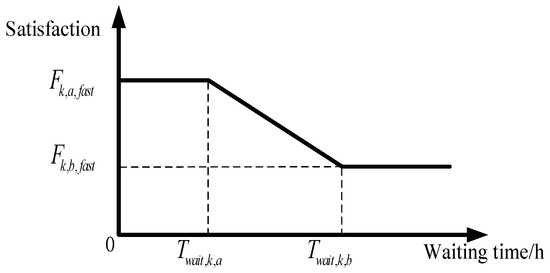
Figure 1.
Relationship between the fast-charging user’s satisfaction and waiting time.
Fast-charging users’ satisfaction with CS planning is reflected in charging queue times, with longer queues resulting in lower satisfaction as follows:
where and are the waiting time at CS c and the satisfaction level of fast-charging user k in choosing CS c; and are the upper and lower limits of satisfaction level of fast-charging user k; and and are the critical queuing times corresponding to the upper and lower limits of satisfaction level. In this paper, the M/G/K model is introduced to describe the charging queuing time of fast-charging users as follows [15]:
where is the expectation of the interval time between arrivals at CS c, is the variance of service time of CS c, are the service time and expectation of CS c, and is the number of fast-charging piles at CS c.
As shown in Figure 2, slow-charging users’ satisfaction with the CS planning is reflected in the availability of vacant slow-charging piles when they arrive, and if so, the satisfaction level is high; otherwise, the satisfaction level is low, as follows:
where is the satisfaction of slow-charging user k in choosing CS c, , and
are the upper and lower limits of satisfaction of slow-charging user k, respectively. The above model can characterize the impact of CS planning results on the charging satisfaction of fast- and slow-charging users, which lays the foundation for the subsequent establishment of a multi-type CS planning model that takes into account the comprehensive satisfaction of users.
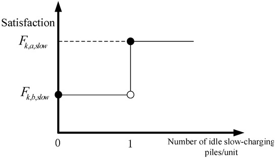
Figure 2.
Relationship between slow-charging user’s satisfaction and the number of free slow-charging piles.
3. A Two-Tier Planning Model for Multi-Type CSs Considering Comprehensive Satisfaction of EV Users
When CSs are equipped with different types of charging piles, planning their locations and the number of each type of charging pile configured has proven to be a challenging task. Meanwhile, the results of CS planning exert notable impacts: they affect both the operation and scheduling of the coupled electric transportation network and the charging satisfaction of users with different types of EVs. To address these considerations, this section establishes a two-layer planning model for multi-type CSs that takes into account the comprehensive satisfaction of users.
The model framework is shown in Figure 3:
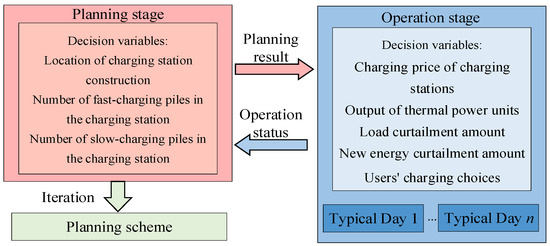
Figure 3.
Framework for two-level planning of multi-type CSs.
In the planning stage, the CS construction location and the number of fast- and slow-charging piles to be constructed in the power traffic coupling network are determined, so as to minimize the planning cost of the CS. Then, building on the planning results and actual operation schemes, optimal scheduling is conducted for the power-transport coupling network. This scheduling process identifies key operational parameters, such as the charging price of each CS under different schemes, the output of thermal power units, the amount of load curtailment, the volume of new energy curtailment, and the temporal and spatial charging choices of fast-charging and slow-charging users. Through this, the operating cost of the power-transport coupling network and the charging satisfaction of fast-charging and slow-charging users are optimized in an integrated manner.
3.1. Upper-Level Planning Optimization Model
3.1.1. Optimization Objective of Upper-Level Model
The upper-level optimization objectives are CS construction costs and operation and maintenance costs.
where is the sum of the construction cost and operation and maintenance cost of the CS, i.e., the total planning cost, and are the construction cost and operation and maintenance cost of the CS, and and y are the discount rate and planning years. The CS construction cost includes fixed investment cost, charging pile purchase cost, and cost related to charging pile power as follows:
where and are the CS infrastructure costs and charging pile purchase costs; and and are the total power-related costs and cost factors, such as the cost of distribution transformers, cables, and other facilities. and are the number of fast- and slow-charging piles constructed, and are the purchase cost of individual fast- and slow-charging piles, and is the number of optional station areas.
The operation and maintenance costs of CSs are positively correlated with the construction costs, and the operation and maintenance costs are calculated as follows:
where is the CS O&M cost factor.
3.1.2. Constraints of Upper-Level Model
The constraints of the upper-level planning model include the following: the number of CSs constraint, the number of charging piles constraint, and the CS capacity constraint as follows:
(1) Constraints on the number of CSs to be built:
The two-tier planning model for multiple types of CSs considering comprehensive user satisfaction developed in this chapter will plan the construction locations of CSs, i.e., a determined number of stations will be selected for construction at several alternative locations to optimize the planning operation cost. Therefore, the constraints on the number of CSs to be constructed are as follows:
where is a binary variable indicating whether region c was selected as a construction site, indicates that it was selected as a construction site, indicates that it was not selected as a construction site, and is the number of CSs constructed.
(2) Charging pile construction quantity constraint:
Due to the minimum configuration requirements of CSs, land capacity, and other factors, this paper considers the following constraints on the number of charging piles to be constructed within a CS:
where and are the upper and lower limits of the number of charging piles at CS c; and are the upper and lower limits of the number of fast-charging charging piles to be constructed at CS c; and and are the upper and lower limits of the number of slow-charging charging piles to be constructed at CS c.
(3) CS capacity constraints:
Due to the coupled power and transportation network relationship, the planning of CSs is also subject to grid operational constraints, i.e., the total charging power of the CSs is limited by the actual carrying capacity of the grid, which is constrained as follows:
where is the upper limit of the total charging power.
3.2. Lower-Level Scheduling Optimization Model
The lower-level scheduling optimization model takes one year as the operation cycle and carries out optimal scheduling based on the planning results of the power-transportation coupling network. In order to reduce the model solving time, and at the same time consider the uncertainty of the operation of the power-transportation coupling network, the lower dispatch optimization model selects several typical days in a year as the optimal scheduling schemes. The model optimizes multiple factors under different schemes, including the charging price of each CS, the output of thermal power units, the amount of purchased power, the amount of new energy curtailment, and the spatio-temporal charging choices of fast- and slow-charging users. Its goal is to achieve comprehensive optimization of the operating cost of the power-transportation coupling network and the charging satisfaction of fast- and slow-charging users for each typical day. The optimization objectives and constraints of the model are as follows:
3.2.1. Optimization Objective of Lower-Level Model
The lower-level scheduling model takes the combined optimal operating cost of the coupled power-transportation network and the charging satisfaction of fast- and slow-charging users as the optimization objective.
where is the total operating cost, is the grid operating costs, is the TN operating costs, and is the user charging satisfaction costs.
Grid operating costs include thermal power unit operating costs, purchased power costs, new energy abandonment costs, and network loss costs, as described below:
where is the number of typical days, is the cost coefficient of thermal unit output, is the number of thermal units, is the actual output of the eth thermal unit, is the price of purchasing reserve power, is the amount of electricity purchased, and are the number of wind farms and photovoltaic (PV) module, and are the cost coefficient of wind power and PV curtailment, and are the curtailed power of the wind farm PV, is the set of grid branches, is the cost coefficient of network losses, is the resistance value of branch xy, and is the square of the current of branch xy.
The cost of operating the transportation network is the cost of roadway congestion penalties, defined as follows:
where is the set of roads in the transportation network, ij represents the road connecting node i and node j in the transportation network, is the road congestion penalty cost coefficient, and is the saturation level of road ij at the moment t.
In order to achieve the goal of keeping the cost of operating the electric transportation coupling network as low as possible while keeping the user charging satisfaction as high as possible, the user satisfaction cost is defined as the negative of the product of the user satisfaction and the user satisfaction cost coefficient. It is specified as follows:
where is the cost coefficient of satisfaction, is the charging satisfaction of the kth user at moment t of the th typical day, and is the number of EVs.
3.2.2. Constraints of Lower-Level Model
The constraints of the lower-level scheduling optimization model include the following: charging price constraints, fast-charging user charging time and space selection constraints, slow-charging user charging time and space selection constraints, user charging state judgment constraints, charging load constraints, current balance constraints, unit operation constraints, new energy reduction constraints, traffic network saturation constraints, and user satisfaction constraints. Among them, the fast-charging user charging time and space selection constraints are shown in Equations (1)–(5), the slow-charging user charging time and space selection constraints are shown in Equations (7)–(9), the user satisfaction constraints are shown in Equations (10)–(12), and the remaining constraints are as follows:
(1) User charging state judgment constraints are as follows:
where = 1 means the EV is in charging status, and = 0 means it is not in charging status. is the starting charging time of the EV, and is the charging duration of the EV.
(2) Charge price constraints
The charging price constraint modeled in this paper is that the charging price at different moments in each CS during each typical day fluctuates up and down based on a determined price curve, and the average charging price is equal to that charging curve, as follows:
where is the average charging price of all CSs at the moment t of the th typical day, is the charging price downward adjustment factor for CSs, is the charging price upward adjustment factor for CSs, and is the charging price of CS c at the moment t.
(3) Charging load constraints are as follows:
where is the active load of CS c at time t of the th typical day, is the charging power chosen by EV user k, is a binary variable indicating whether user k chooses CS c for charging at time t, with 1 indicating a choice and 0 indicating a non-choice, is the time set of user’s willingness to charge on the th typical day, is a binary variable indicating whether user k chooses to charge in hour t, where 1 indicates choice and 0 indicates non-choice, is a binary variable indicating whether user k is in charging state after choosing for charging time and at CS c, where 1 indicates a state of charging and 0 indicates a state of not being in charging, is the reactive power load of CS c at time t, and is the power factor.
(7) Transportation network saturation constraints are as follows:
where is a binary variable indicating whether user k chooses to charge at CS c and passes by at time t, where 1 means passes by and 0 means not, is the set of roads that user k who chooses to charge at CS c and passes by at time t, is the saturation level of road ij on the th typical day at time t, and is the traffic volume of road ij on the th typical day at time t, which excludes dispatched EVs, and is the number of EVs that are supported by road ij at time t, and is the number of EVs that are supported by road ij at time t, which does not include dispatched EVs. Traffic volume excludes dispatched EVs, is a binary variable indicating whether user k on the th typical day chooses to charge at time t or not, where a value of 1 indicates a choice and a value of 0 indicates a non-choice, and is the load capacity of the feeder road ij.
In addition to the above constraints, the second stage model also needs to consider tidal flow constraints, nodal balancing, and unit operation constraints, which are not discussed here.
4. Solving Algorithm
The lower-layer scheduling optimization model of the multi-type CS two-layer planning model established in this paper, which considers the comprehensive satisfaction of users, contains a large number of binary variables related to EV users, and if it is directly substituted into the upper-layer model to solve the problem in a unified way, the complexity of the model rises sharply with the increase in the typical day and the number of EV users, which leads to the difficulty of the model to be applied to the real world.
Therefore, this section introduces a greedy algorithm-based solution for the two-layer planning model. The main reason for adopting this strategy is that direct integration of the upper-layer siting and configuration decisions with the lower-layer scheduling, both containing large numbers of binary variables, would lead to excessive computational complexity. The greedy approach reformulates the problem into a multi-round expansion process, where each iteration adds charging piles based on sensitivity coefficients. This reduces dimensionality, accelerates convergence, and preserves the logical interaction between planning and scheduling. Consequently, the algorithm not only ensures computational tractability but also yields solutions that balance cost, user satisfaction, and practical feasibility.
4.1. Solution Strategy for Two-Layer Planning Model Based on Greedy Algorithm
The sensitivity factor is first defined as the ratio of the difference between the optimal operating cost of the two rounds of iteration and the difference between the optimal total planning cost of the two rounds of iteration, as follows:
where and are the sensitivity coefficients and the optimal cost of the mth iteration, and is the optimal total planning cost of the mth iteration.
Each round of iteration generates a set of scenarios under the premise of satisfying the constraints on the number of charging piles to be constructed and the capacity constraints of CSs, and each scenario adds a number of fast-charging piles or a number of slow-charging piles to the optimal scenarios obtained in the previous round.
4.2. Steps for Solving the Two-Layer Planning Model Based on the Greedy Algorithm
The greedy algorithm-based solution process for the two-tier planning model is described as follows:
Step 1: Initialize the parameters to generate an initial set of planning scenarios based on the lower limit of the number of charging piles to be constructed;
Step 2: Delete the planning schemes that do not satisfy the constraints on the number of charging piles to be constructed and the capacity of CSs to be constructed from the scheme set. If the number of remaining schemes is greater than 0, go to step 3; otherwise, go to step 5;
Step 3: Substitute the planning scenarios in the scenario set into the lower-level scheduling optimization model and calculate the sensitivity coefficient of each scenario. If the highest sensitivity coefficient is greater than 0, go to step 4; otherwise, go to step 5;
Step 4: Update the set of scenarios with the highest sensitivity coefficient, go to step two;
Step 5: Output the optimal solution obtained from the previous iteration. If the solution satisfies the CS construction constraints, output the planning scheme and end; otherwise, go to step 6;
Step 6: Find the CS with the lowest number of charging pile plans in the previous iteration and make that CS no longer a pending CS, and return to step 1.
5. Case Studies
5.1. Scene Setting
In this paper, the validity of the proposed model is verified by taking the IEEE 33-node test system and the 27-node urban traffic network system as an example, which is shown in Figure 4. There are three CSs located at nodes 3, 7, and 10 of the TN, and connected to nodes 20, 4, and 31 of the EN, and there are 60 fast-charging piles and 15 slow-charging piles. There are three sites to be constructed, two of which are selected to build CSs, located at nodes 14, 16, and 26 of the TN, connected to nodes 23, 33, and 11 of the EN, with at least 16 fast-charging piles and 4 slow-charging piles in each CS, and at most 50 fast-charging piles and 25 slow-charging piles. Node 24 of the grid has a wind farm with a capacity of 35 MW, nodes 17, 21, 32, and 33 each have a micro-fuel unit with a capacity of 500 kW, and node 33 is connected to the main grid for purchasing backup power from the main grid. The urban TN includes 2000 EVs, of which 1800 are fast-charging users and 200 are slow-charging users, with a battery capacity of 82 kWh and a travel speed of 40 km/h. The charging pile has a fast-charging power of 45 kW and a slow-charging power of 7 kW, with a power factor of 0.95. The slow-charging users are classified into three categories according to their travel characteristics, and the charging position of each category of slow-charging user in the TN in the morning and evening is shown in Table 1.
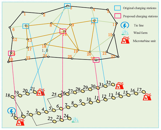
Figure 4.
IEEE 33-Bus test system and 27-Bus TN system.

Table 1.
Charging position in the morning and evening for each type of slow-charging users.
In this paper, based on the historical data of wind power output and load in a region of Anhui Province, the wind power output and the active-reactive power load of four typical days in spring, summer, fall, and winter are sampled and generated, as shown in Figure 5, Figure 6 and Figure 7. Here, t represents the time period, measured in hours. Specifically, t is a discrete index indicating the time slot within the day. Among them, the active-reactive load is the load sum of 33 nodes, and the load data of each node are generated based on the load data of the IEEE 33-node test system and the load data of typical days. Three key parameters are generated with reference to relevant studies: the initial charge state of both fast-charging and slow-charging users, the time when fast-charging users enter the traffic network, and the traffic volume of the traffic network on each typical day [16,17,18].
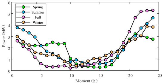
Figure 5.
Wind power output at each moment of typical days.
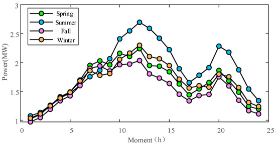
Figure 6.
Active power load output at each moment of typical days.
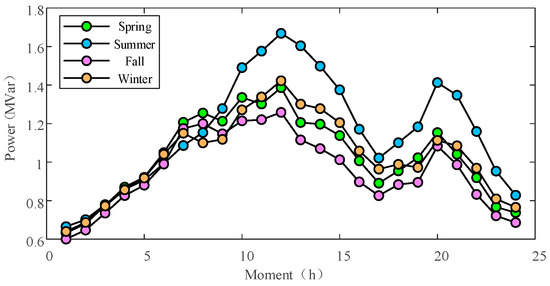
Figure 7.
Reactive power load output at each moment of typical days.
In this paper, the fixed construction cost of CS is set to be CNY 1 million (Chinese Yuan), the operation and maintenance cost is 0.3 times the construction cost [19], the construction cost of the fast-charging pile is CYN 20,000, the construction cost of the slow-charging pile is CNY 5000, the equivalent investment coefficient related to the total power of the CS is 0.13, the average discount rate is 0.085, and the operating life is 20 years. The cost parameters for the construction and operation of the charging station are shown in Table 2. The average charging price at each moment of the CS is shown in Figure 8, the cost of each type of generation is shown in Table 3, the road congestion penalty cost coefficient is set to 100, and the user satisfaction cost coefficient is set to 0.3.
Table 2.
Charging Station Construction and Operation Cost Parameters.
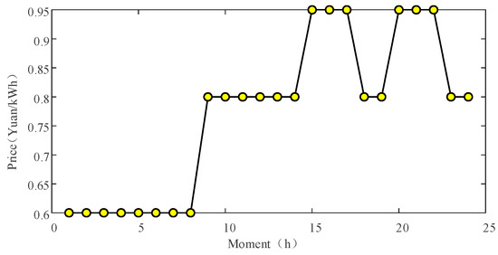
Figure 8.
Average charging price of CSs at each moment.
Table 3.
Various cost coefficients.
5.2. Analysis of the Effectiveness of the Coupled Electric Traffic Network Planning Model
In order to verify the effectiveness of the planning model proposed in this paper, the location of the CS and the number of fast and slow charging is optimized based on the model of this paper, and the planning scheme and the comparative analysis scheme are obtained as shown in Table 4, of which Scheme 1 relies only on the original CS to serve the users; Scheme 2 is the planning scheme obtained by the optimization model in this chapter; Scheme 3 chooses the same construction location with Scheme 2, and changes the ratio of fast and slow charging in the CS and increases the number of charging piles in the station; and Schemes 4 and 5 have the same fast and slow-charging ratios as in Scheme 2 and change the construction location of the CS. Table 5 shows the planning costs and the annual operating costs of the electric traffic coupling network for each planning scheme.
Table 4.
Set of planning programs for model validity analysis.
Table 5.
Planning and annual operating costs of the program.
Compared with Scheme 2, all the operating costs of Scheme 1 are at a disadvantage, and its operating costs are much larger than those of Scheme 2, indicating that the construction of CSs can optimize the actual operation of the coupled electric traffic network.
Compared to Scheme 2, Scheme 3 increases the planned number of charging piles, so that the charging satisfaction of users is improved in actual operation. The annual wind abandonment cost and network loss cost of Scheme 3 have been reduced because the CSs located at node 14 of the traffic network are close to the wind farms, and the increased charging capacity of the CSs promotes the consumption of wind power and reduces the transmission loss of electric energy at the same time. However, the annual power purchase cost and the annual micro fuel unit cost of this option have increased, while the planning cost has greatly increased, resulting in the actual economics of Option 3 being inferior to that of Option 2.
Compared with Scheme 2, Scheme 4 adjusts the planning result of 16 nodes to 26 nodes, and Scheme 5 adjusts the result of 14 nodes to 16 nodes and 16 nodes to 26 nodes, resulting in the need for the vehicle to travel to CSs farther away from the wind farm to charge, and although the cost of wind abandonment decreases at this time, more power is lost in transmission, and the cost of network losses rises significantly. At the same time, the annual power purchase cost and the annual cost of micro-fuel generation are also correspondingly elevated. The result is that Scheme 4 and 5 are not as economical to operate in practice as Scheme 2.
Meanwhile, comparing the schemes, it can be seen that the cost of road congestion penalties and user satisfaction have changed under different schemes, but the change is small, which is related to the selection of the cost coefficients, and a detailed analysis will be carried out in this section in the subsequent examples of calculations.
In summary, the model in this paper is able to achieve both the optimal allocation of the number of fast and slow charging, to ensure the economy of the planning scheme while considering the satisfaction of the user, and to achieve the selection of the CS location, to enhance the operational efficiency of the power traffic coupling network.
5.3. Analysis of the Impact of the Planning Program on the Operation of EN
The following is an analysis of the optimization effect of the planning scheme obtained through the planning model on the operation of the power grid. Based on the model in this chapter, the location of CSs and the number of fast and slow chargers are optimized, and the planning scheme and the comparative analysis scheme are obtained as shown in Table 6, in which Scheme a(1) is the planning scheme obtained from the model in this chapter; Scheme a(2) has the same construction location and different fast and slow-charging ratios in the CSs compared to Scheme a(1); and Scheme a(3) has the same fast and slow-charging ratios in the CSs compared to Scheme a(2), with different construction locations of CSs. The construction location of CS is different.
Table 6.
Set of planning programs.
Figure 9, Figure 10 and Figure 11 show the charging loads for different planning schemes on a typical day in summer, and Figure 12, Figure 13 and Figure 14 show the corresponding grid scheduling results. CS1, CS2, CS3, CS4, and CS5 in Schemes a(1) and a(2) correspond to CSs at nodes 3, 7, 10, 14, and 16 of the traffic network, and CS1, CS2, CS3, CS4, and CS5 in Scheme a(3) correspond to CSs at nodes 3, 7, 10, 16, and 26 of the traffic network.
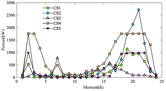
Figure 9.
CSs load at each moment of Program a(1).
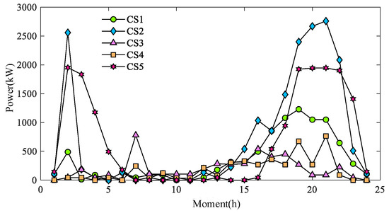
Figure 10.
CSs load at each moment of Program a(2).
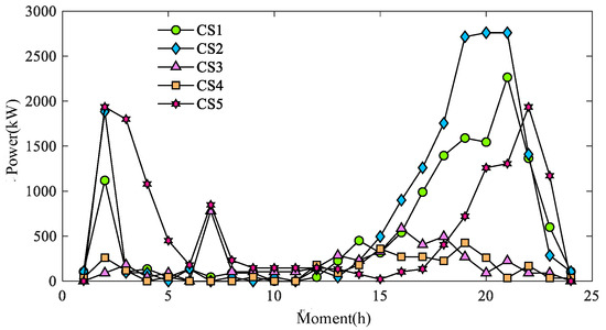
Figure 11.
CSs load at each moment of Program a(3).
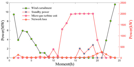
Figure 12.
Power grid scheduling results of Program a(1).
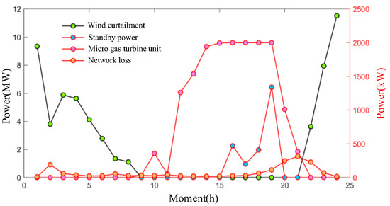
Figure 13.
Power grid scheduling results of Program a(2).
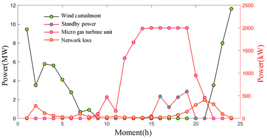
Figure 14.
Power grid scheduling results of Program a(3).
First, a comparison is made for Scheme a(1) and Scheme a(2), where the same location is chosen for the construction of the CS for both schemes, but the capacity of the CS differs. Comparing the 17–19 h when the grid scheduling results are more different, it can be seen from the figure that the purchased reserve power under Scheme a(2) is elevated in these hours compared to Scheme a(1), and rises sharply in the 19 h. This is due to the fact that the maximum charging capacity of CS2, which is close to the wind farm in Scheme a(2), has decreased, and some users have shifted to CS1, 2, and 5, which have larger capacities, to charge in order to improve their charging satisfaction. Due to the time slot difference between the user charging decision and performing charging, a large number of charging loads are gathered at 19 h, which makes it necessary to purchase more standby power at 19 h to satisfy the grid power demand. Meanwhile, CS2 charging load rises at 17–19 h, causing more power to flow from the power source to the grid node 4, resulting in some elevation of network losses in the corresponding time period. Compared with Scheme a(1), Scheme a(2) adds 837 kW of spare power dispatch and 333 kW of network losses in intraday operation.
Then, a comparison is made between Schemes a(1) and a(3), which differ in terms of both the siting and capacity of CSs. Comparing the 2 h and 7 h, where the grid scheduling results are more different, it can be seen that the wind power curtailment under Scheme a(3) in these periods is reduced compared to Scheme a(1), but the network loss is increased. This is due to the fact that the maximum charging capacity of the CSs close to the wind farms and the liaison lines has decreased and the maximum capacity of the CSs connected to the grid 11 node has increased in Scheme a(3) compared to Scheme a(1), resulting in the transfer of some of the users to CS5 for charging in the a(3) Scheme. This leads to a load rise at the grid 11 nodes at 2 h and 7 h, causing the grid to increase network losses while utilizing more wind power for energy supply. Compared to Scheme a(1), Scheme a(3) increases network losses by 895 kW in intraday operation, but also reduces wind power curtailment by 1412 kW.
In summary, the impact of the siting and capacity of EV CSs on grid operation is reflected in the transfer of EV charging loads between different nodes, which in turn has an impact on the operational scheduling results of the grid.
5.4. Analysis of Impacts of Planning Scenarios on TN Operations
The following is a comparative analysis of the scenarios in Table 7 to analyze the difference between the planning scenarios obtained by the planning method for optimizing the operation of the traffic network under different parameter settings. In particular, Scheme b(1) is the planning scheme obtained when the congestion penalty factor is set to 100, and Scheme b(2) is the planning scheme obtained when the congestion penalty factor is set to 1,000,000. Scheme b(1) operates at a saturation level of 550.1254 on a typical day, and Scheme b(2) at 548.6376.
Table 7.
Set of planning programs for traffic network impact analysis.
Figure 15 and Figure 16 show the number of EVs passing each road at each moment under different schemes, respectively, and it can be seen that the number of vehicles passing each road decreases in most of the roads in Scheme b(2) compared to Scheme b(1), with the most significant change at 1 h. Figure 17 shows a comparison of the decrease in the number of vehicles passing each road and the road capacity for Scheme b(2) compared to Scheme b(1) at 1 h.
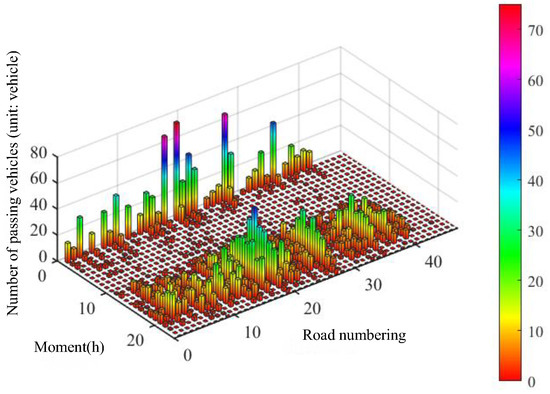
Figure 15.
Number of EVs passing through each road of Scheme b(1).
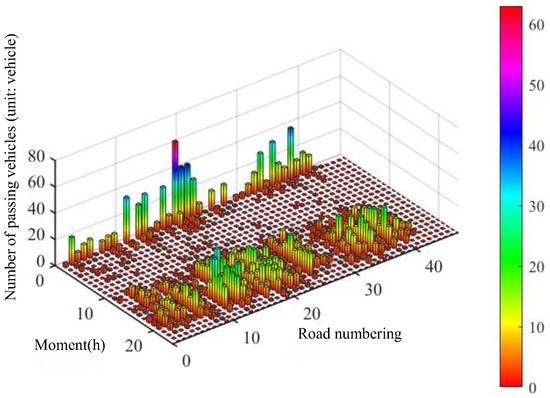
Figure 16.
Number of EVs passing through each road of Scheme b(2).
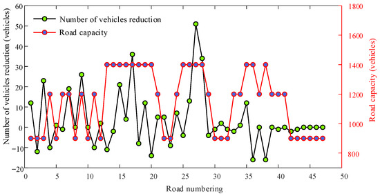
Figure 17.
Comparison of 1 h EV count decline and road capacity.
It is observed that the number of EVs passing by the vast majority of roads in 1 h decreased, while the number of EVs passing by a few roads increased. Among the 10 roads where the number of passing EVs increased, only 2 roads have a capacity of 900, 4 of the remaining 8 have a capacity of 1200, and the other 4 have a capacity of 1400. This indicates that differences in planning scenarios affect the users’ choice of CSs, which in turn changes their path of travel while charging, ultimately affecting traffic flow.
In summary, different planning schemes will affect the user’s choice of CS, which will affect the traffic flow. By adjusting the road congestion penalty coefficient in the model of this paper, different planning schemes can be obtained, and the planning scheme with a large coefficient has a stronger regulating effect on TN.
5.5. Analysis of the Impact of the Planning Program on User Satisfaction
The following is a comparative analysis of the scenarios in Table 8 to analyze the difference between the planning scenarios obtained by the planning method under different parameter settings for user satisfaction optimization. Scheme c(1) is the planning scheme obtained when the satisfaction cost coefficient is set to 0.3; Scheme c(2) is the planning scheme obtained when the satisfaction cost coefficient is set to 3. Compared with Scheme c(1), Scheme c(2) expands the number of fast-charging piles constructed at each CS, and the number of slow-charging piles decreases. The user satisfaction is 116,170 for Scheme c(1) and 117,970 for Scheme c(2) operating under a typical day.
Table 8.
Set of planning programs for satisfaction impact analysis.
Figure 18 and Figure 19 show the charging load of CSs for different schemes under a typical day, where CS1, CS2, CS3, CS4, and CS5 in Schemes c(1) and c(2) correspond to CSs at nodes 3, 7, 10, 14, and 16 of TN.
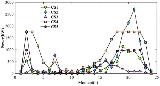
Figure 18.
CSs load at each moment of Program c(1).
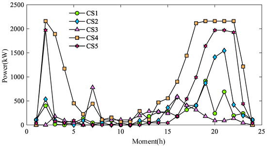
Figure 19.
CSs load at each moment of Program c(2).
The difference between Schemes c(1) and c(2) is mainly in the fact that the charging capacity of the CS5 rises in c(2), which improves the charging satisfaction of the fast-charging users who traveled to the CS5. Comparison of Figure 18 and Figure 19 shows that the charging load of CS5 in 19–22 h is greatly increased in c(2), indicating that more users went to CS5 for charging at this time, and at the same time, the fast-charging users’ satisfaction with CS5 increased under this scheme, which led to an increase in the overall user satisfaction.
Figure 20 shows the improvement of comprehensive user satisfaction with algorithm iteration in the process of solving the optimal charging pile configuration after determining the planning location under different schemes. From the figure, it can be seen that compared with Scheme c(1), c(2) still improves user satisfaction at the later stage of iteration in the planning process. This is because compared with Scheme c(1), c(2) sets a larger satisfaction cost coefficient, and the solution algorithm proposed in this paper tends to select the sub-scheme that makes the biggest improvement in the comprehensive user satisfaction in each iteration round.
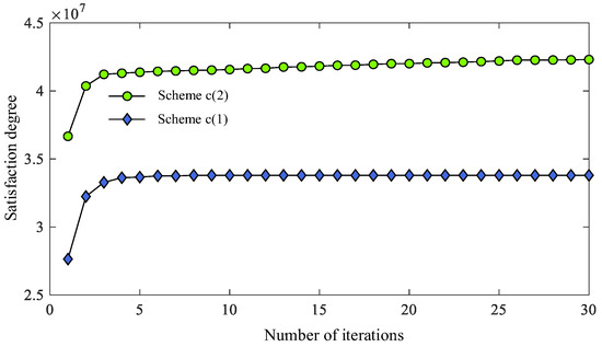
Figure 20.
Iterative curve of comprehensive user satisfaction of different programs.
To summarize, different planning schemes affect user charging satisfaction, which in turn changes the user’s charging choice. The planning scheme obtained by the proposed method is able to maximize the user’s comprehensive satisfaction while ensuring that the scheme cost is minimized. Different planning schemes can be obtained by adjusting the satisfaction cost coefficient in the model. When the coefficient is larger, the planning scheme can obtain better comprehensive user satisfaction in actual operation, while the algorithm also selects the sub-scheme with better user satisfaction in each round of iteration.
6. Conclusions
This paper proposes a collaborative planning model for multi-type CSs considering comprehensive user satisfaction. Firstly, a comprehensive satisfaction model of multi-type charging loads considering user behavioral characteristics is established; secondly, a two-layer planning model of multi-type CSs considering user comprehensive satisfaction is established to optimize the location of CSs and the number of fast and slow-charging configurations in the stations; thirdly, a two-layer planning model solution based on the greedy algorithm is proposed for the model solving problem; finally, an example analysis is carried out to verify the proposed model. Finally, an example analysis is carried out to verify the effectiveness of the proposed model. The conclusions are summarized as follows:
- (1)
- The planning scheme proposed in this paper is able to consider the comprehensive charging satisfaction of users while considering the actual operating costs of the electric traffic coupling network, and results in a planning scheme with optimal planning and operating economics;
- (2)
- The impact of EV CS siting and capacity setting on grid operation is reflected in the transfer of EV charging loads between different nodes of the grid, which in turn has an impact on the operation and scheduling results of the grid, and achieves the purpose of promoting new energy consumption and reducing network losses;
- (3)
- The location and capacity of EV CSs will have an impact on the degree of road congestion in TN and on the comprehensive satisfaction of users, and adjusting the road congestion penalty coefficient and the satisfaction cost coefficient can make the obtained scheme have a greater advantage in traffic congestion alleviation and improve the comprehensive satisfaction of users.
Author Contributions
Methodology, X.Y., F.Z. and Y.M.; software, Y.Z. and R.X.; validation, Y.Z. and R.X.; data curation, C.R. and C.Z.; writing—original draft preparation, C.R. and C.Z. All authors have read and agreed to the published version of the manuscript.
Funding
This work was supported by the Science and Technology Project of State Grid Anhui Electric Power Co., Ltd. (No. B3120924000G).
Data Availability Statement
The original contributions presented in this study are included in the article. Further inquiries can be directed to the corresponding author.
Conflicts of Interest
Authors Xin Yang, Fan Zhou, Yalin Zhong and Ran Xu were employed by the State Grid Anhui Economic Research Institute. The remaining authors declare that the research was conducted in the absence of any commercial or financial relationships that could be construed as a potential conflict of interest.
Nomenclature
| Constants | |
| Pfast | Fast-charging pile power |
| Pslow | Slow-charging pile power |
| M | An arbitrarily large positive number used in operations |
| α | Charging price downward adjustment factor |
| β | Charging price upward adjustment factor |
| λCS | Discount rate used in CS construction cost |
| c | Index for CS location |
| k | Index for user (EV) |
| n | Number of charging piles |
| Twait | Waiting time for charging at a CS |
| Variables | |
| Fk,fast | Satisfaction level of fast-charging user k at a given CS |
| Fk,slow | Satisfaction level of slow-charging user k at a given CS |
| y | Binary variable indicating whether user k is charging in time period t |
| Sk | State of charge for user k at time t |
| Ck | Charging capacity of user k |
| Dk | Distance for user k to the nearest CS location |
| TCS | Charging time of the CS |
| LoadCS | The charging load of CS cc at time t |
| CostCS | The cost incurred by the CS for operation |
| Satisfaction Cost | A cost associated with user satisfaction |
| Tk | The time taken for user k to charge |
| Wk | Waiting time of user k at the CS |
| PEV | Power drawn by the EV user during charging |
| Functions | |
| fCS(t) | Charging load function at time t for CS c |
| gwait(t) | Waiting time function for users at time t |
| fuser(k) | User charging function that determines the charging time, location, and pile selection for user k |
| hcost(k,c) | Cost function for user k at CS c |
| fload(t) | Load function used for scheduling in the network |
| Abbreviations | |
| EV | Electric Vehicle |
| CS | Charging Station |
| O&M | Operation and Maintenance |
| TN | Traffic Network |
| EN | Electric Network |
| M/G/K Model | A model used to describe queuing time for fast-charging users |
| PEV | Plug-in Electric Vehicle |
| PV | Photovoltaic |
References
- He, Y.; Wu, H.; Wu, A.Y.; Li, P.; Ding, M. Optimized shared energy storage in a peer-to-peer energy trading market: Two-stage strategic model regards bargaining and evolutionary game theory. Renew. Energy 2024, 224, 120190. [Google Scholar] [CrossRef]
- Zulfiqar, M.; Abdeen, Z.; Kamran, M. Optimizing electric vehicle charging scheduling using enhanced multi-agent neural networks with dynamic pricing. J. Energy Storage 2024, 99, 113317. [Google Scholar] [CrossRef]
- Sun, Z.; He, Y.; Wu, H.; Wu, A.Y. Bi-level planning of electric vehicle charging stations considering charging demand: A Nash bargaining game approach. Energy 2025, 332, 137137. [Google Scholar] [CrossRef]
- Zhang, H.; Moura, S.J.; Hu, Z.; Song, Y. PEV fast-charging station siting and sizing on coupled transportation and power networks. IEEE Trans. Smart Grid 2018, 9, 2595–2605. [Google Scholar] [CrossRef]
- Shukla, A.; Verma, K.; Kumar, R. Planning of fast charging stations in distribution system coupled with transportation network for capturing EV flow. In Proceedings of the 2018 8th IEEE India International Conference on Power Electronics, Jaipur, India, 13–15 December 2018; pp. 1–6. [Google Scholar]
- Wang, W.; Liu, Y.; Wei, W.; Wu, L. A bilevel EV charging station and DC fast charger planning model for highway network considering dynamic traffic demand and user equilibrium. IEEE Trans. Smart Grid 2024, 15, 714–728. [Google Scholar] [CrossRef]
- Lu, H.; Xie, K.; Shao, C.; Hu, B.; Pan, C.; Huang, B. Charging Station Planning with the Dynamic and Mixed Traffic Flow of Gasoline and Electric Vehicles. High Volt. Eng. 2023, 49, 1150–1160. [Google Scholar]
- Chen, Z.; Wan, Y.; Hu, Z.; Li, J. District and County Level Electric Vehicle Fast Charging Station Planning Considering Stochastic User Equilibrium. Autom. Electr. Power Syst. 2024, 48, 25–34. [Google Scholar]
- Mao, D.; Tan, J.; Wang, J. Location planning of PEV fast charging station: An integrated approach under traffic and power grid requirements. IEEE Trans. Intell. Transp. Syst. 2021, 22, 483–492. [Google Scholar] [CrossRef]
- Zhang, M.; Zhang, Q.; Yang, X. Joint planning of electric vehicle fast charging stations and distribution network based on a traffic-electricity equilibrium coupling model. Power Syst. Prot. Control 2023, 51, 51–63. [Google Scholar]
- Cao, F.; Hu, J. Destination-driven EV Fast Charging Station Capacity Configuration. In Proceedings of the 2021 IEEE 5th Conference on Energy Internet and Energy System Integration, Taiyuan, China, 22–24 October 2021; pp. 22–24. [Google Scholar]
- Tao, Y.; Qiu, J.; Lai, S.; Sun, X.; Zhao, J. Adaptive integrated planning of electricity networks and fast charging stations under electric vehicle diffusion. IEEE Trans. Power Syst. 2023, 38, 499–513. [Google Scholar] [CrossRef]
- Jiang, Z.; Han, J.; Li, Y.; Chen, X.; Peng, T.; Xiong, J.; Shu, Z. Charging station layout planning for electric vehicles based on power system flexibility requirements. Energy 2023, 283, 128983. [Google Scholar] [CrossRef]
- Li, Y.; Su, S.; Liu, B.; Yamashita, K.; Li, Y.; Du, L. Trajectory-driven planning of electric taxi charging stations based on cumulative prospect theory. Sustain. Cities Soc. 2022, 86, 104125. [Google Scholar] [CrossRef]
- Zhang, W.; Chen, L.; Huang, Y.; Niu, L.; Huang, M.; Zhang, D.; Shi, W. Application of M/G/k Queuing Model in Queuing System of Electric Taxi Charging Station. Power Syst. Technol. 2015, 39, 724–729. [Google Scholar]
- Shao, Y.; Mu, Y.; Yu, X.; Dong, X.; Jia, H.; Wu, J.; Zeng, Y. Spatial-temporal Charging Load Forecast and Impact Analysis Method for Distribution Network Using EVs-Traffic-Distribution Model. Proc. CSEE 2017, 37, 5207–5219. [Google Scholar]
- Sreekumar, A.; Lekshmi, R. Electric vehicle charging station demand prediction model deploying data slotting. Results Eng. 2024, 24, 103095. [Google Scholar] [CrossRef]
- Liao, Q.; Li, G.; Yu, J.; Gu, Z.; Ma, W. Online prediction-assisted safe reinforcement learning for electric vehicle charging station recommendation in dynamically coupled transportation-power systems. Transp. Res. Part C Emerg. Technol. 2025, 176, 105155. [Google Scholar] [CrossRef]
- Xiao, B.; Gao, F. Optimization method of electric vehicle charging stations’ site selection and capacity determination considering charging piles with different capacities. Electr. Power Autom. Equip. 2022, 42, 157–166. [Google Scholar]


Disclaimer/Publisher’s Note: The statements, opinions and data contained in all publications are solely those of the individual author(s) and contributor(s) and not of MDPI and/or the editor(s). MDPI and/or the editor(s) disclaim responsibility for any injury to people or property resulting from any ideas, methods, instructions or products referred to in the content. |
© 2025 by the authors. Licensee MDPI, Basel, Switzerland. This article is an open access article distributed under the terms and conditions of the Creative Commons Attribution (CC BY) license (https://creativecommons.org/licenses/by/4.0/).