Abstract
Sulfate radicals are increasingly recognized for their potent oxidative capabilities, making them highly effective in degrading persistent organic pollutants (POPs) in aqueous environments. These radicals excel in breaking down complex organic molecules that are resistant to traditional treatment methods, addressing the challenges posed by POPs known for their persistence, bioaccumulation, and potential health impacts. The complexity of predicting interactions between sulfate radicals and diverse organic contaminants is a notable challenge in advancing water treatment technologies. This study bridges this gap by employing a range of machine learning (ML) models, including random forest (DF), decision tree (DT), support vector machine (SVM), XGBoost (XGB), gradient boosting (GB), and Bayesian ridge regression (BR) models. Predicting performances were evaluated using R2, RMSE, and MAE, with the residual plots presented. Performances varied in their ability to manage complex relationships and large datasets. The SVM model demonstrated the best predictive performance when utilizing the Morgan fingerprint as descriptors, achieving the highest R2 and the lowest MAE value in the test set. The GB model displayed optimal performance when chemical descriptors were utilized as features. Boosting models generally exhibited superior performances when compared to single models. The most important ten features were presented via SHAP analysis. By analyzing the performance of these models, this research not only enhances our understanding of chemical reactions involving sulfate radicals, but also showcases the potential of machine learning in environmental chemistry, combining the strengths of ML with chemical kinetics in order to address the challenges of water treatment and contaminant analysis.
1. Introduction
Sulfate radicals are known for their potent oxidative capabilities, making them an attractive agent for the degradation of persistent organic pollutants in aqueous environments [1]. These radicals are highly reactive, enabling them to break down complex organic molecules that are otherwise resistant to conventional treatment methods. This effectiveness is particularly crucial in addressing the challenge posed by persistent organic contaminants (POPs), which are known for their persistence, bioaccumulation, and potential adverse health effects. Studies have shown that sulfate radicals are more selective and show higher reactivity toward electron-rich pollutants; they can effectively degrade a wide range of these pollutants, including pharmaceuticals [2,3], personal care products [4], and industrial chemicals [5,6], often achieving higher degradation rates than other advanced oxidation processes. Furthermore, the generation of sulfate radicals can be achieved through various environmentally benign methods, notably through the homogenous activation of persulfate (PS) or peroxymonosulfate (PMS) using heat, ultraviolet (UV) light, base, or transition metals [7], thereby enhancing their appeal for sustainable water treatment technologies [8]. This aligns with the increasing global emphasis on green chemistry and sustainable solutions for environmental pollution.
Given the widespread use of SO4−• in the elimination of organic contaminates, obtaining the reaction rate constant is crucial for designing effective water treatment systems and for a comprehensive understanding of the underlying chemical mechanisms; however, considering the huge amount of chemicals is time consuming and requires extensive laboratory work to figure out the reaction kinetics of each chemical [9]. Neta et al. [10] measured the second-order rate constants (k) for the reaction of SO4−• with various substituted benzenes and benzoates, ranging from approximately 105 to 109 M−1 s−1. Nguyen et al. [11] tested the second-order rate coefficients for the aqueous SO4−• with a series of organic aerosol compounds, such as 2-methyltetrol, 2-methyl-1,2,3-trihydroxy-4-sulfate, 2-methyl-1,2-dihydroxy-3-sulfate, and so on, which assisted the understanding the aerosol mass sinks. Therefore, predicting the reaction rate constants of organic contaminants toward sulfate radicals is essential, for it not only represents a significant leap in environmental chemistry, but is also a pragmatic step towards the optimization of water treatment processes. Accurate predictions enable us to prioritize and regulate the use of sulfate radicals based on the reactivity of different pollutants, thus streamlining the treatment process.
Quantitative structure−activity relationship (QSAR) models provide a valuable predictive framework, correlating chemical structure with reactive tendencies, and thus reducing the need for extensive empirical experimentation [12]. This methodology was applied to predict the toxicity [13] and activity [14,15] of chemicals. Sudhakaran et al. [16] developed QSAR models for ozonation and the •OH oxidation of organic micropollutants to predict kO3 and k•OH based on multi-linear regression, resulting the R2 > 0.75, and identified descriptors like double bond equivalence (DBE), ionization potential (IP), and electron affinity (EA) to affect k to different extents. Song et al. [3] built prediction models toward the kinetic constants of a suit of 15 PPCPs, incorporating model parameters such as the steady state of the radical concentration; moreover, the potential error induced by other radicals, such as CO3•−, Br•−,were also taken into consideration, necessitating extensive laboratory work.
Traditional QSAR analysis employs predefined mathematical models and molecular descriptors, often requiring domain expertise for feature selection and generally offering clearer interpretability. However, it is less flexible and may struggle with complex, non-linear data. The complexity of chemical reactions in environmental matrices often outstrips the capacity of traditional QSAR models to provide rapid and accurate predictions. This complexity is compounded by the vast number of potential contaminants and the variability of environmental conditions, which can alter reaction dynamics. Machine learning models emerge as a necessary evolution in this field, offering the ability to assimilate large datasets and uncover patterns.
To address these limitations and harness the complexity of chemical interactions, numerous machine learning (ML) models were developed and employed in the environmental field. These ML models were utilized across different scenarios to predict environmental problems, including forecasting regional daily to yearly PM2.5 variations [17,18], predicting the change of various wastewater variables [19,20]. More specifically, Lu et al. developed multilayered neural network (NN) models to forecast the temperature-dependent site-specific rate constants of hydroxyl radical reactions with alkanes [21]; the results showed that the proposed NN models are robust in predicting the site-specific and overall rate constants. Not only used for prediction, ML models can also assist in classification, Cheng et al. [22] trained five different ML models to classify 3486 per- and polyfluoroalkyl substances (PFASs) from the OECD list, the multitask neural network, and graph-based models demonstrated the best performance. Generally, ensemble models like XGBoost (XGB) and gradient boosting (GB) models often perform well on a wide range of problems, but can be complex [23], while simple models like decision trees (DTs) are interpretable [24], but prone to overfitting. The selection of different machine learning models based on task demands is crucial to achieving robust prediction results.
Inspired by the recent successes in ML modeling in environmental chemistry, we investigate the efficacy of six distinct ML models—random forest, decision tree, support vector machine, XGB, GB, and Bayesian ridge regression—in the prediction of the reaction constants of organic contaminants with SO4−•; the data were collected from peer-reviewed papers. These models spanning various categories including ensemble methods (RF, XGB, GB), predictive modeling (DT), discriminative models (SVM), and regularized regression (BR). Although there are already several studies on the prediction of the rate constant of organic contaminants mediated by sulfate radicals [25,26], this study compared the performances of six different machine learning models and two different features (Morgan-type fingerprints and chemical descriptors). Model performances were estimated by internal and external validation using R2, RMSE, and MAE. Residual plots were presented to evaluate the ML performance. The SHAP values determined the top 10 important features. By applying these models to predict the reaction constants of organic contaminants with SO4−•, our study aims to compare six machine learning models in order to identify the most effective approach for predicting the reaction constants of organic contaminants with SO4−•. By employing two distinct feature types, we seek to evaluate which feature set provides more accurate and reliable predictions.
The novelty of our research lies in the comprehensive comparison of six distinct machine learning models. Furthermore, both Morgan fingerprints and chemical descriptors have been applied as predictive features. Through this combination of Ml models and chemical analysis, our research aims to establish the predictive modeling of reaction rates, offering insights that could revolutionize water treatment methodologies and our understanding of the fate of environmental pollutants.
2. Data Collection and Model Construction
2.1. Data Sets and MF
The reaction rate constants for the oxidative processes targeting a suit of organic contaminants, mediated by SO4−• radicals, were compiled from the peer-reviewed literatures [27,28,29,30,31,32,33,34,35,36], focusing on studies where the pH ranged from 5.5 to 7.5, and temperatures were within 20–25 °C. In certain studies, authors reported rate constants with k values. To normalize skewed distributions and reduce the impact of outliers, the data were transformed to the logarithmic scale when necessary, thereby enhancing the model accuracy and interpretability. The InChIKeys and SMILES codes for these chemicals were extracted via web crawling techniques from PubChem. This method ensured comprehensive and efficient data collection but was limited by the reliability and structure of the source websites. In instances where multiple reaction rate constants were reported for the same chemical, the average value was utilized. This approach, chosen to provide a representative rate constant for each chemical, potentially introduces a level of approximation, but is necessary to manage data variability. Following pre-cleaning, 724 chemicals, each accompanied by its corresponding experimental logk values, were used in model development. Using the RDKit program, these SMILES codes were converted into Morgan fingerprints, along with 209 chemical descriptors [37]. For some compounds lacking certain chemical descriptors, this resulted in ‘nan’ values in the dataset, potentially leading to errors in the model construction. To maintain data integrity and ensure model accuracy, these ‘nan’ values were systematically dropped from the dataset using the Python ‘dropna’ method. Following this data cleaning step, the dataset was reduced to 716 chemicals for analysis, applying chemical descriptors as features.
In the Morgan fingerprint analysis, a series of scans were conducted to determine the optimal length of the MF, with values including 512, 1024, 2048, 3072, 4096, and 8192. After selecting the fingerprint length yielding the optimal predictive performance, features were reduced through the following procedures: (1) dropping columns with a standard deviation greater than 0.1. This threshold was chosen as features with low variability (lower standard deviation) are less informative for models, and their removal can reduce noise and prevent overfitting. (2) Another method included calculating Pearson parameters and eliminating columns with Pearson correlations exceeding 0.96 [38]. This step was crucial to remove multicollinearity, as highly correlated features can distort the importance of variables and reduce the generalizability of the model. Following this methodology, we narrowed down the features to 168 chemical characteristics, deemed most relevant and robust for further model development. The entire database can be accessed via the file “SupInfoDataSet.xlsx”, available in the Supporting Information section. This database comprises four sheets: “3072 MorganMFs” and “Chemical Descriptors”, which, respectively detail the 3072-bit Morgan molecular fingerprints and chemical features of each chemical, generated using RDKit. The “Morgan MFs_test_train set” and “CDs_train_test set” sheets display the experimental and gradient boosting model-predicted logKSO4−• values, based on the 3072-bit Morgan MFs and chemical features, respectively.
2.2. Hyperparameter Optimization
A fivefold grid search was conducted for hyperparameters optimization [39]. This approach is advantageous as it allows for a comprehensive assessment of how different hyperparameter settings impact the model’s performance, leading to the identification of an optimal set that enhances prediction accuracy. A range of values were considered, and the optimal hyperparameters were determined using the mean R2 value on the validation set (Table 1). The hyperparameters across models, such as n_estimators (number of trees) and max_depth (tree depth) for ensemble methods like random forest and XGBoost, control model complexity and overfitting. In SVM, the Kernel determines the data transformation, C balances the classification accuracy and simplicity, and gamma affects the influence range of a single sample. For gradient boosting, learning_rate adjusts the contribution of each tree, enhancing performance tuning. In Bayesian ridge regression, alpha_1 and lambda_1 manage model complexity, while n_iter influences the convergence speed, collectively fine-tuning the balance between the model accuracy and generalization. The selected ranges for each hyperparameter were chosen based on their potential impact on model performance, with a focus on achieving an optimal balance between accuracy and generalizability. The final optimized hyperparameters for each model were also presented.

Table 1.
Hyperparameters used for different models.
2.3. ML Models and Validation
Six machine learning algorithms—random forest (RF), decision tree (DT), support vector machines (SVM), XGBoost (XGB), Bayesian ridge regression (BR), and gradient boosting (GB)—were utilized for predicting the reaction rate constant in the interactions between sulfate radicals and organic chemicals. These were selected for their diverse strengths and proven capabilities in various predictive modeling scenarios, ranging from capturing non-linear relationships to handling high-dimensional data. These predictive models were developed using scikit-learn packages [40]. Datasets were randomly split into an 80% training set and a 20% test set. Both internal and external validations were implemented to ascertain the reliability and robustness of the ML models, as well as their predictive capacity. Performance indices—correlation coefficient (R2), root-mean-square deviation (RMSE), and mean absolute error (MAE)—were computed. The concurrent application of these metrics in both training and testing phases facilitated a comprehensive evaluation. Specifically, RMSE underscored the model’s sensitivity to substantial errors, and MAE offered a direct estimation of average errors [40]. This dual approach steered the models towards a more balanced and resilient optimization.
2.4. Model Interpretation
A fundamental principle in developing QSAR/QSPR models is the mechanistic interpretation of the model, which necessitates predictions anchored in essential chemical interpretations [41]. In the realm of molecular descriptors, selected physicochemical properties are pivotal for optimal predictions. In this context, the SHapley Additive exPlanations (SHAP) method, an advanced interpretive technique, was employed to elucidate predictions. SHAP, renowned for elucidating machine learning model predictions by attributing feature importance values in the context of all possible feature combinations [42,43], was utilized to enhance our model’s interpretability. By employing SHAP, we identified and visualized the top ten critical features to our predictions through violin plots, shedding light on the significant factors that drive the predictive performance. This approach not only underscores the importance of transparent model interpretation, but also aids researchers in pinpointing the essential features that govern the prediction of reaction rate constants, thereby enriching our model’s explanatory power.
3. Results and Discussion
3.1. Effects of the MF Length
In this study, MFs are essential for converting molecular structures into fixed-length binary vectors, thereby enabling the quantitative assessment of molecular similarities and differences. This feature is vital for accurately and efficiently modeling molecular properties. To determine the optimal MF length that balances predictive performance with computational efficiency in the Morgan type, a preliminary study was undertaken. The R2 of the test set was selected to evaluate the predicting performances; Figure 1 illustrates how the R2 values were influenced by varying the length of MFs across different models. It was observed that longer MF lengths typically yield improved predictive performance for the tested models, except for the DT model. The variability in the performance of the DT model can be indicative of overfitting when provided with an increasingly complex feature space, a known limitation of decision trees. The selection of the optimal MF length was thus guided by a balance between maximizing predictive accuracy and maintaining computational efficiency. After evaluating the performance across various lengths, a 3072-bit length was chosen as the optimal size. This decision was based on its robust performance in enhancing R2 values across models, without disproportionately increasing computational demands. While lengths beyond 3072 bits did show some incremental improvements in R2, these were marginal and did not justify the significantly higher computational costs involved. Hence, 3072 bits was established as the optimal length for MFs in our study.
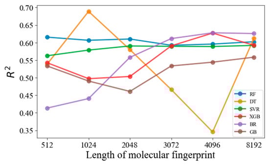
Figure 1.
Effect of the Morgan fingerprint length on the R2 values of selected machine learning models.
3.2. Internal and External Validation
The ML models generated R2train values in the range of 0.922~0.988 when using Morgan fingerprints (3072 bits) as features, suggesting good fitting of the training set (Table 2). To further assess the reliability of the developed models, external validation was performed using R2test as statistical criteria. The R2test was used to measure the correlation between experimental and predicted logk values; an R2 value of 1 indicated that the regressions perfectly fit the data. In this study, the values ranged from 0.532~0.712. The SVM model has the lowest MAE and RMSE on both the training and test sets, which are crucial metrics for generalization, showing the smallest average error in the predictions. The results demonstrate that SVM methods emerge as the top-performing model for this particular task when using the R2test as the scoring factor. Contrastingly to the SVM model, the XGB and GB models yielded R2test values higher than 0.97 and R2test values higher than 0.60. Both have small MAE and RMSE numbers in their test sets, which demonstrated a robust predicting performance. BR also showed R2train values higher than 0.98 and R2test values around 0.597; however, when comparing with boosting models, we can see higher MAE and RMSE results on both the training and test sets. The results revealed that the ensemble and boosting methods (XGB, BR, GB) consistently outperformed the single models (DT) on both training and test sets [44]. Previous research also demonstrated that an ensemble is on generally more accurate than single base models [45].
Table 2.
The performance parameters of machine learning models on training and test sets, using Morgan fingerprints.
Table 2 details the performance parameters of these models; our analysis revealed that ensemble and boosting methods consistently outperformed single models, aligning with the existing literature that suggests that ensemble approaches generally achieve higher accuracy than individual base models. The p-values for each pair of machine learning models, based on the R2test values derived from tenfold cross validation, were also calculated. The SVM model showed a significant difference with the rest of the models (p < 0.05), except for the gradient boost model (p = 0.032).
When choosing a model for tasks requiring high accuracy and reliability, like predicting reaction constants, the model should balance between fitting the training data and generalizing the unseen data. For example, the SVM model’s robust performance underscores its suitability for complex predictive tasks, where minimizing errors is crucial. On the other hand, the high R2train and R2test scores of the XGB and GB models, combined with their low error metrics, highlight their potential in capturing the underlying patterns within the data without overfitting, making them reliable choices for predicting the reaction constants in varied chemical environments.
The predicted versus experimental logk values are presented in Figure 2; the diagonal dash represented the r = 1. The scatter being closer to this line indicated a better predicting performance; contrarily, the scatter far away from the diagonal indicated a bias between the predicted and experimental values. It is evident that the SVM, XGB, and GB models exhibit a high concentration of points near the diagonal, indicating a strong correlation between the predicted and experimental values. This suggests that these models have a higher predictive accuracy. However, there are some noticeable outliers, particularly in the DT model, where a few points significantly stray from the line of perfect correlation. These outliers indicate instances where the DT model failed to predict the logk values accurately, possibly due to the model’s inability to capture complex patterns within the data.
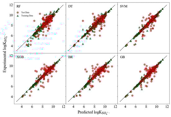
Figure 2.
Plots of the predicted logk values from Morgan MFs versus the experimental values of both training and test sets.
The results calculated for models built on chemical descriptors are presented in Table 3. Considering the evaluated performance metrics, XGB and GB models exhibited the highest R2 scores on both the training and test sets; this is consistent with the results displayed in Table 2. Specifically, the R2 values exceeded 0.99 on the training set, and 0.8 for the test set, underscoring a superior predictive performance with chemical descriptors as features.
Table 3.
The performance parameters of machine learning models on training and test sets using chemical descriptors.
The GB model, in particular, showcased strong generalization capabilities across the training and test sets, displaying the lowest error metrics in the test set. Conversely, while the DT and SVM models perform well on the training set, a marked decrease in performance on the test set suggests overfitting. In contrast, the XGB model achieves the highest R2 score on the training set and sustains this high level of performance on the test set, indicative of its excellent predictive ability with consistently low error rates. The BR model, however, exhibits the lowest performance on the training set and shows minimal improvement on the test set; this is indicative of potential underfitting or an inability to capture the dataset’s complexity adequately. Statistical analyses for each pair of machine learning models based on the R2test values derived from tenfold cross validation revealed that the GB model was statistically significantly different from the other four models (p < 0.05), only presenting similarity to the RF model (p = 0.648).
In light of these results, the GB and XGB models emerge as the most dependable for deployment, characterized by high R2 and low error metrics on unseen data, suggesting that they effectively capture the underlying data patterns without overfitting. Similar research from Li et al. [46] utilized different types of ML models to predict the net ecosystem carbon exchange. They also observed that the gradient boosting regression model was more accurate when compared to the other three models (support vector machine, stochastic gradient descent, and Bayesian ridge). Dineva et al. compared the ensemble boosting and bagging models for ground water potential prediction. The results revealed that bagging models like RF outperformed boosting models [47]. Such findings underscore the necessity of choosing the appropriate model based on the specific predictive task at hand, as no single approach fits all scenarios.
The logk values, as predicted from chemical descriptors verses experimental values, are presented in Figure 3. In XGB and GB models, the scatters showed high density proximate to the diagonal, indicating good predicting performances. The RF model shows a reasonable alignment with the diagonal and has a slightly more dispersed pattern, hinting at variability in its predictive accuracy. The DT model exhibits a more pronounced spread of points, which suggests a lesser degree of predictive accuracy when compared to the XGB and GB models. On the other hand, a notable pattern is observed in the SVM model plot where the predicted points align vertically along an axis. This alignment is a visual indicator of poor predictive performance, as the model predictions do not vary with the changes in the experimental logk values, resulting in a lack of correlation.
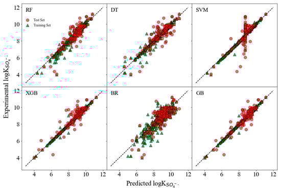
Figure 3.
Plots of the predicted logk values from chemical descriptors versus experimental values of both training and test sets.
The differences between the observed and predicted values, known as residuals, are plotted against the predicted values in order to assess the performance of machine learning models [48]. Residual plots were created for gradient boosting models (Figure 4), which use Morgan fingerprints and chemical descriptors as features, respectively. The residuals in these models are randomly distributed across all predicted values, indicating effective prediction performance. When using MFs as features, there is a wider spread of residuals, especially in predictions ranging from eight to nine. Conversely, when featured as chemical descriptors, the residuals scatter evenly around the horizontal axis, demonstrating a strong fit without noticeable systematic errors. Most residuals lie within a −1 to 1 range, reflecting minor prediction errors, with only a few outliers. Both models show a concentration of residuals near zero, but the gradient boosting model, which utilizes chemical descriptors, exhibits a denser clustering around zero, thus signifying greater accuracy.
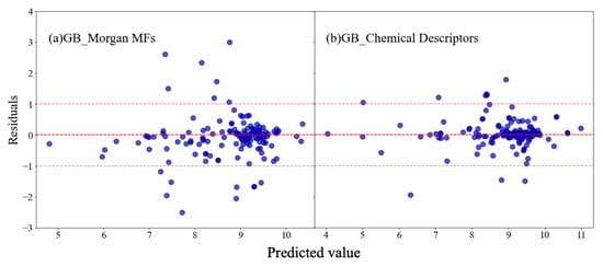
Figure 4.
Residual plots of (a) the gradient boosting model established on MFs and (b) chemical descriptors, respectively. (The red dashed lines at residuals equals −1, 0 and 1 respectively represented reference lines to help evaluate the distribution of residuals in our model).
3.3. SHapley Additive exPlanations (SHAP) Analysis
SHAP analysis is a method developed to interpret machine learning models by quantifying the impact of each feature on the model’s prediction. This approach provides a foundation for understanding the contribution of individual features to predictive outcomes, offering transparency in model decision-making processes. In this study, SHAP analysis was conducted, as presented in Figure 5. It illustrated a SHAP summary plot for GB models which use Morgan fingerprints and chemical descriptors, respectively, which quantify the contribution of individual features to the predictive outcomes. Each dot represents a SHAP value for a feature and an instance; the position on the x-axis indicates the impact of that value on the model’s output. Features are ordered vertically by the sum of SHAP value magnitudes across all samples, which indicates the overall importance of the feature. The color gradient signifies the magnitude and direction of the feature’s effect, with one end of the spectrum (blue) representing low feature values, and the other end (red) representing high values. A feature’s value that pushes the prediction to the right of the mid line suggests an increased likelihood of the higher outcome predicted by the model, while a shift to the left indicates a lower outcome. In this study, Morgan fingerprints of 2897 bits and a chemical feature of SMR_VSA7 were the most impactful features effecting the prediction outcome. It offers insights into molecular volume and its potential impact on reactivity and interaction with biological targets. Chi3v was the second important chemical feature; it captures the complexity of molecular structures by quantifying the connectivity of atoms within a molecule, which can influence molecular stability and reactivity. This is followed by Balaban J, which provides a quantitative insight into the molecular complexity, which can affect molecular properties such as reactivity and biological activity [37]. SHAP analysis provides insights into the feature importance and their individual contributions to the model’s predictive capabilities. The top ten impactful chemical descriptors and their description are presented in Table 4.
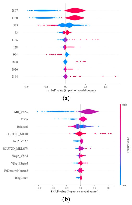
Figure 5.
Importance of the top ten representative MF features (a) and chemical descriptors (b) and their impact on the model output for the Gradient Boosting model applied to logk.
Table 4.
The top ten impactful features and their descriptions from SHAP analysis.
To summary, a 3072-bit length was identified as the optimal MF length, balancing the predictive accuracy with computational efficiency. Ensemble and boosting methods, such as XGB and GB, consistently outperformed single models, aligning with the literature on the efficacy of ensemble approaches in achieving higher accuracy. Additionally, SHAP analysis provided insights into the importance of individual features in the model predictions, highlighting the significance of specific molecular features like SMR_VSA7 and Chi3v on the outcome. Comprehensive analysis and significant findings were detailed in the conclusion section.
4. Conclusions
This study employed six different machine learning models combined with Morgan molecular fingerprints and chemical features to develop prediction models for sulfate radicals-induced oxidation rate constants. The model performances were dependent on fingerprint length; for BR, XGB, and GB models, the R2 value slightly decreased and then increased as the length was extended. For the SVM and RF models, which were not sensitive to the MF length, the R2 remained relatively stable as the length of the MFs changed. For Morgan fingerprints, the SVM models demonstrated robust generalization capabilities, achieving the highest R2 on the test set. For chemical descriptors, the GB and XGB models emerged as the most reliable for deployment, exhibiting high R2 and low error metrics on the test data, indicating their effectiveness in capturing the underlying data patterns without overfitting. Models based on chemical features generally performed better than those based on Morgan fingerprints. SHAP analysis was conducted, and Morgan fingerprint bit 2897, along with the descriptor SMR_VSA7, were identified as the dominant features affecting the prediction performance. This study suggests the practicality of utilizing machine learning approaches to predict the reaction rate of organic contaminants in response to sulfate radicals, while also uncovering influential physical/chemical properties related to reaction rates. It also highlighted the importance of selecting appropriate machine learning models and features to achieve robust prediction performances.
Supplementary Materials
The following supporting information can be downloaded at: https://www.mdpi.com/article/10.3390/pr12020384/s1.
Author Contributions
Conceptualization, T.T. and G.L.; methodology, T.T.; software, T.T.; validation, D.S., J.C. and Z.C.; formal analysis, Y.D.; investigation, T.T.; resources, G.L.; data curation, T.T.; writing—original draft preparation, T.T.; writing—review and editing, T.T. and G.L.; visualization, D.S., J.C. and Z.C.; supervision, G.L. and Z.D.; project administration, T.T., G.L. and Z.D.; funding acquisition, T.T. All authors have read and agreed to the published version of the manuscript.
Funding
This research was supported by National Science Fund of China for Young Scholars [42107409], China postdoctoral Science Foundation [2021M701247] and GuangZhou Basic and Applied Basic Research Foundation [202201010223].
Data Availability Statement
The raw data supporting the conclusions of this article will be made available by the authors on request.
Conflicts of Interest
The authors declare no conflict of interest.
References
- Giannakis, S.; Lin, K.-Y.A.; Ghanbari, F. A review of the recent advances on the treatment of industrial wastewaters by Sulfate Radical-based Advanced Oxidation Processes (SR-AOPs). Chem. Eng. J. 2021, 406, 127083. [Google Scholar] [CrossRef]
- Hassani, A.; Scaria, J.; Ghanbari, F.; Nidheesh, P. Sulfate radicals-based advanced oxidation processes for the degradation of pharmaceuticals and personal care products: A review on relevant activation mechanisms, performance, and perspectives. Environ. Res. 2023, 217, 114789. [Google Scholar] [CrossRef] [PubMed]
- Lian, L.; Yao, B.; Hou, S.; Fang, J.; Yan, S.; Song, W. Kinetic study of hydroxyl and sulfate radical-mediated oxidation of pharmaceuticals in wastewater effluents. Environ. Sci. Technol. 2017, 51, 2954–2962. [Google Scholar] [CrossRef] [PubMed]
- Nfodzo, P.; Choi, H. Sulfate radicals destroy pharmaceuticals and personal care products. Environ. Eng. Sci. 2011, 28, 605–609. [Google Scholar] [CrossRef]
- Li, W.; Orozco, R.; Camargos, N.; Liu, H. Mechanisms on the impacts of alkalinity, pH, and chloride on persulfate-based groundwater remediation. Environ. Sci. Technol. 2017, 51, 3948–3959. [Google Scholar] [CrossRef] [PubMed]
- Yang, M.; Ren, X.; Hu, L.; Guo, W.; Zhan, J. Facet-controlled activation of persulfate by goethite for tetracycline degradation in aqueous solution. Chem. Eng. J. 2021, 412, 128628. [Google Scholar] [CrossRef]
- Ji, Y.; Wang, L.; Jiang, M.; Lu, J.; Ferronato, C.; Chovelon, J.-M. The role of nitrite in sulfate radical-based degradation of phenolic compounds: An unexpected nitration process relevant to groundwater remediation by in-situ chemical oxidation (ISCO). Water Res. 2017, 123, 249–257. [Google Scholar] [CrossRef]
- Lai, J.; Tang, T.; Du, X.; Wang, R.; Liang, J.; Song, D.; Dang, Z.; Lu, G. Oxidation of 1, 3-diphenylguanidine (DPG) by goethite activated persulfate: Mechanisms, products identification and reaction sites prediction. Environ. Res. 2023, 232, 116308. [Google Scholar] [CrossRef]
- Pardue, H.L. Kinetic aspects of analytical chemistry. Anal. Chim. Acta 1989, 216, 69–107. [Google Scholar] [CrossRef]
- Neta, P.; Madhavan, V.; Zemel, H.; Fessenden, R.W. Rate constants and mechanism of reaction of sulfate radical anion with aromatic compounds. J. Am. Chem. Soc. 1977, 99, 163–164. [Google Scholar] [CrossRef]
- Tran, L.N.; Abellar, K.A.; Cope, J.D.; Nguyen, T.B. Second-Order Kinetic Rate Coefficients for the Aqueous-Phase Sulfate Radical (SO4•–) Oxidation of Some Atmospherically Relevant Organic Compounds. J. Phys. Chem. A 2022, 126, 6517–6525. [Google Scholar] [CrossRef] [PubMed]
- Nirmalakhandan, N.N.; Speece, R.E. QSAR model for predicting Henry’s constant. Environ. Sci. Technol. 1988, 22, 1349–1357. [Google Scholar] [CrossRef]
- Agrawal, V.; Khadikar, P. QSAR prediction of toxicity of nitrobenzenes. Bioorg. Med. Chem. 2001, 9, 3035–3040. [Google Scholar] [CrossRef] [PubMed]
- Du, Q.-S.; Huang, R.-B.; Chou, K.-C. Recent advances in QSAR and their applications in predicting the activities of chemical molecules, peptides and proteins for drug design. Curr. Protein Pept. Sci. 2008, 9, 248–259. [Google Scholar] [CrossRef]
- Xiao, R.; Ye, T.; Wei, Z.; Luo, S.; Yang, Z.; Spinney, R. Quantitative Structure-Activity Relationship (QSAR) for the Oxidation of Trace Organic Contaminants by Sulfate Radical. Environ. Sci. Technol. 2015, 49, 13394–13402. [Google Scholar] [CrossRef]
- Sudhakaran, S.; Amy, G.L. QSAR models for oxidation of organic micropollutants in water based on ozone and hydroxyl radical rate constants and their chemical classification. Water Res. 2013, 47, 1111–1122. [Google Scholar] [CrossRef] [PubMed]
- Hu, X.; Belle, J.H.; Meng, X.; Wildani, A.; Waller, L.A.; Strickland, M.J.; Liu, Y. Estimating PM2. 5 concentrations in the conterminous United States using the random forest approach. Environ. Sci. Technol. 2017, 51, 6936–6944. [Google Scholar] [CrossRef]
- Gupta, P.; Christopher, S.A. Particulate matter air quality assessment using integrated surface, satellite, and meteorological products: Multiple regression approach. J. Geophys. Res. Atmos. 2009, 114, D20205. [Google Scholar] [CrossRef]
- Zhu, J.-J.; Anderson, P.R. Performance evaluation of the ISMLR package for predicting the next day’s influent wastewater flowrate at Kirie WRP. Water Sci. Technol. 2019, 80, 695–706. [Google Scholar] [CrossRef]
- Haimi, H.; Mulas, M.; Corona, F.; Vahala, R. Data-derived soft-sensors for biological wastewater treatment plants: An overview. Environ. Model. Softw. 2013, 47, 88–107. [Google Scholar] [CrossRef]
- Lu, J.; Zhang, H.; Yu, J.; Shan, D.; Qi, J.; Chen, J.; Song, H.; Yang, M. Predicting Rate Constants of Hydroxyl Radical Reactions with Alkanes Using Machine Learning. J. Chem. Inf. Model. 2021, 61, 4259–4265. [Google Scholar] [CrossRef]
- Cheng, W.; Ng, C.A. Using Machine Learning to Classify Bioactivity for 3486 Per- and Polyfluoroalkyl Substances (PFASs) from the OECD List. Environ. Sci. Technol. 2019, 53, 13970–13980. [Google Scholar] [CrossRef]
- Kavzoglu, T.; Teke, A. Predictive Performances of ensemble machine learning algorithms in landslide susceptibility mapping using random forest, extreme gradient boosting (XGBoost) and natural gradient boosting (NGBoost). Arab. J. Sci. Eng. 2022, 47, 7367–7385. [Google Scholar] [CrossRef]
- Yin, G.; Jameel Ibrahim Alazzawi, F.; Mironov, S.; Reegu, F.; El-Shafay, A.S.; Lutfor Rahman, M.; Su, C.-H.; Lu, Y.-Z.; Chinh Nguyen, H. Machine learning method for simulation of adsorption separation: Comparisons of model’s performance in predicting equilibrium concentrations. Arab. J. Chem. 2022, 15, 103612. [Google Scholar] [CrossRef]
- Ding Han, H.j. Prediction of Second-Order Rate Constants of Sulfate Radical with Aromatic Contaminants Using Quantitative Structure-Activity Relationship Mode. Water 2021, 14, 766. [Google Scholar] [CrossRef]
- Sanches-Neto, F.O.; Dias-Silva, J.R.; Keng Queiroz Junior, L.H.; Carvalho-Silva, V.H. “pySiRC”: Machine Learning Combined with Molecular Fingerprints to Predict the Reaction Rate Constant of the Radical-Based Oxidation Processes of Aqueous Organic Contaminants. Environ. Sci. Technol. 2021, 55, 12437–12448. [Google Scholar] [CrossRef]
- Fabio Mercado, D.; Bracco, L.L.B.; Argues, A.; Gonzalez, M.C.; Caregnato, P. Reaction kinetics and mechanisms of organosilicon fungicide flusilazole with sulfate and hydroxyl radicals. Chemosphere 2018, 190, 327–336. [Google Scholar] [CrossRef] [PubMed]
- Gabet, A.; Metivier, H.; Brauer, C.d.; Mailhot, G.; Brigante, M. Hydrogen peroxide and persulfate activation using UVA-UVB radiation: Degradation of estrogenic compounds and application in sewage treatment plant waters. J. Hazard. Mater. 2021, 405, 124693. [Google Scholar] [CrossRef] [PubMed]
- Wang, Z.; Shao, Y.; Gao, N.; Lu, X.; An, N. Degradation of diethyl phthalate (DEP) by UV/persulfate: An experiment and simulation study of contributions by hydroxyl and sulfate radicals. Chemosphere 2018, 193, 602–610. [Google Scholar] [CrossRef] [PubMed]
- Rickman, K.A.; Mezyk, S.P. Kinetics and mechanisms of sulfate radical oxidation of β-lactam antibiotics in water. Chemosphere 2010, 81, 359–365. [Google Scholar] [CrossRef] [PubMed]
- Gupta, S.; Basant, N. Modeling the reactivity of ozone and sulphate radicals towards organic chemicals in water using machine learning approaches. RSC Adv. 2016, 6, 108448–108457. [Google Scholar] [CrossRef]
- Real, F.J.; Acero, J.L.; Benitez, J.F.; Roldan, G.; Casas, F. Oxidation of the emerging contaminants amitriptyline hydrochloride, methyl salicylate and 2-phenoxyethanol by persulfate activated by UV irradiation. J. Chem. Technol. Biotechnol. 2016, 91, 1004–1011. [Google Scholar] [CrossRef]
- Cvetnic, M.; Stankov, M.N.; Kovacic, M.; Ukic, S.; Bolanca, T.; Kusic, H.; Rasulev, B.; Dionysiou, D.D.; Loncaric-Bozic, A. Key structural features promoting radical driven degradation of emerging contaminants in water. Environ. Int. 2019, 124, 38–48. [Google Scholar] [CrossRef]
- Cvetnic, M.; Tomic, A.; Sigurnjak, M.; Stankov, M.N.; Ukic, S.; Kusic, H.; Bolanca, T.; Bozic, A.L. Structural features of contaminants of emerging concern behind empirical parameters of mechanistic models describing their photooxidative degradation. J. Water Process Eng. 2020, 33, 101053. [Google Scholar] [CrossRef]
- Shi, Y.; Yan, F.; Jia, Q.; Wang, Q. Normindex for predicting the rate constants of organic contaminants oxygenated with sulfate radical. Environ. Sci. Pollut. Res. 2020, 27, 974–982. [Google Scholar] [CrossRef]
- Wojnárovits, L.; Takács, E. Rate constants of sulfate radical anion reactions with organic molecules: A review. Chemosphere 2019, 220, 1014–1032. [Google Scholar] [CrossRef] [PubMed]
- RDKit: Open-Source Cheminformatics. Available online: http://www.rdkit.org (accessed on 10 February 2024).
- Bouwmeester, R.; Martens, L.; Degroeve, S. Comprehensive and Empirical Evaluation of Machine Learning Algorithms for Small Molecule LC Retention Time Prediction. Anal. Chem. 2019, 91, 3694–3703. [Google Scholar] [CrossRef]
- Pedregosa, F.; Varoquaux, G.; Gramfort, A.; Michel, V.; Thirion, B.; Grisel, O.; Blondel, M.; Prettenhofer, P.; Weiss, R.; Dubourg, V. Scikit-learn: Machine learning in Python. J. Mach. Learn. Res. 2011, 12, 2825–2830. [Google Scholar]
- Hodson, T.O. Root-mean-square error (RMSE) or mean absolute error (MAE): When to use them or not. Geosci. Model Dev. 2022, 15, 5481–5487. [Google Scholar] [CrossRef]
- OECD. Guidance Document on the Validation of (Quantitative) Structure-Activity Relationship [(Q) SAR] Models; Organisation for Economic Co-Operation and Development: Paris, France, 2014. [Google Scholar]
- Lundberg, S.; Lee, S. A Unified Approach to Interpreting Model Predictions. ArXiv 2017, arXiv:1705.07874. [Google Scholar]
- Lundberg, S.M.; Erion, G.; Chen, H.; DeGrave, A.; Prutkin, J.M.; Nair, B.; Katz, R.; Himmelfarb, J.; Bansal, N.; Lee, S.-I. From local explanations to global understanding with explainable AI for trees. Nat. Mach. Intell. 2020, 2, 56–67. [Google Scholar] [CrossRef] [PubMed]
- Bourel, M.; Cugliari, J.; Goude, Y.; Poggi, J.-M. Boosting diversity in regression ensembles. Stat. Anal. Data Min. ASA Data Sci. J. 2020, 1–17. [Google Scholar] [CrossRef]
- Odegua, R. An empirical study of ensemble techniques (bagging, boosting and stacking). In Proceedings of the Deep Learning IndabaX. 2019. Available online: https://www.researchgate.net/publication/338681864_An_Empirical_Study_of_Ensemble_Techniques_Bagging_Boosting_and_Stacking (accessed on 10 February 2024).
- Cai, J.; Xu, K.; Zhu, Y.; Hu, F.; Li, L. Prediction and analysis of net ecosystem carbon exchange based on gradient boosting regression and random forest. Appl. Energy 2020, 262, 114566. [Google Scholar] [CrossRef]
- Mosavi, A.; Sajedi Hosseini, F.; Choubin, B.; Goodarzi, M.; Dineva, A.A.; Rafiei Sardooi, E. Ensemble Boosting and Bagging Based Machine Learning Models for Groundwater Potential Prediction. Water Resour. Manag. 2021, 35, 23–37. [Google Scholar] [CrossRef]
- Boldini, D.; Grisoni, F.; Kuhn, D.; Friedrich, L.; Sieber, S.A. Practical guidelines for the use of gradient boosting for molecular property prediction. J. Cheminform. 2023, 15, 73. [Google Scholar] [CrossRef]


Disclaimer/Publisher’s Note: The statements, opinions and data contained in all publications are solely those of the individual author(s) and contributor(s) and not of MDPI and/or the editor(s). MDPI and/or the editor(s) disclaim responsibility for any injury to people or property resulting from any ideas, methods, instructions or products referred to in the content. |
© 2024 by the authors. Licensee MDPI, Basel, Switzerland. This article is an open access article distributed under the terms and conditions of the Creative Commons Attribution (CC BY) license (https://creativecommons.org/licenses/by/4.0/).