Abstract
A major challenge in transient pressure analysis for shale gas wells is their complex transient flow behavior and fracturing parameters. While numerical simulations offer high accuracy, analytical models are attractive for transient pressure analysis due to their high computational efficiency and broad applicability. However, traditional analytical models are often oversimplified, making it difficult to capture the complex seepage system, and three-dimensional fracture characteristics are seldom considered. To address these limitations, this study presents a comprehensive hybrid model that characterizes the transient flow behavior and analyzes the pressure response of a fractured shale gas well with a three-dimensional discrete fracture. To achieve this, the hydraulic fracture is discretized into several panels, and the transient flow equation is numerically solved using the finite difference method. Based on the Langmuir adsorption isotherm and the pseudo-steady diffusion in matrix and Darcy flow in the network of micro-fractures, a reservoir model is established, and the Laplace transformation is adopted to solve the model analytically. The transient responses are obtained by dynamically coupling the flow in the reservoir and the discrete fracture. The precision of the proposed model is validated using the commercial numerical simulator, Eclipse. A series of transient pressure dynamic curves are drawn to make a precise observation of different flow regimes, and the effects of several parameters on transient pressure response are also examined. The results show that the shale gas well testing interpretation curves comprise nine flow stages. The pressure drop of shale gas reservoirs is lower than that of conventional gas reservoirs due to the replenishment of desorbed gas. The artificial fracture flow capacity, fracture length, and height are the main engineering factors affecting the pressure responses of shale gas wells. Maximizing the degree and scope of reconstruction can enhance the gas well production capacity during fracturing construction. The research results also indicate that our model is a reliable semi-analytical model for well test interpretations in real case studies.
1. Introduction
Shale gas is an unconventional natural gas that is primarily found in adsorbed and free states within organic-rich shale and its interbeds [1,2]. Compared to conventional reservoirs, shale reservoirs have poor physical properties and high geostress, and their economic development requires the use of large-scale hydraulic fracturing technology [3,4]. Shale gas reservoirs exhibit different characteristics in terms of permeability and transformation effects, and the distribution characteristics and unstable flow laws of the fracturing network are extremely complex. Accurately describing the distribution and characteristics of the fracturing network and evaluating the effective fracture length and flow parameters are prerequisites for optimizing hydraulic fracturing design and developing shale gas efficiently [5,6,7]. Therefore, establishing a pressure dynamic analysis method for the three-dimensional hydraulic fracturing network of shale gas is of great significance for understanding the flow law of the fracturing network and obtaining pressure dynamic responses.
Shale gas reservoirs are a special type of gas reservoir that differ significantly from conventional gas reservoirs in terms of their formation, occurrence, and flow mechanisms. Due to the complex multi-scale storage and permeability spaces and diverse occurrence modes of shale gas reservoirs, gas flow exhibits corresponding multiple flow mechanisms during the flow process [8,9,10]. However, current research on the complex flow mechanisms of shale gas reservoirs is not systematic and lacks consideration of the influence of three-dimensional fracture networks. Well testing, as a dynamic monitoring “eye”, is an effective means of obtaining key flow parameters of shale reservoirs and fracture networks and clarifying the dynamic changes in shale pressure [11,12,13]. Analytical and semi-analytical models require only a few grids to be assigned to the fracture, which significantly reduce the number of grids and increase the computational efficiency [14,15,16,17,18,19]. Currently, the most commonly used shale gas well testing interpretation models are SRV models and discrete fracture models [20,21,22,23]. However, the traditional analytical models are limited to two-dimensional flow problems and seldom consider the three-dimensional distribution and characteristics of the fracture network, leading to considerable errors in pressure dynamic analysis. Numerical methods, such as finite difference, finite element, and finite volume, can effectively handle the flow problem of three-dimensional fractures [1,24,25,26]. However, when using these methods for well testing analysis, many problems may occur. The process of establishing such fracture networks using commercial numerical simulation software is relatively complex. In addition, the use of localized refinement or non-uniform grids can lead to an increase in the number of grids and significant differences in size between grids, thereby substantially reducing calculation efficiency. Therefore, there is a need to carry out relevant research on the three-dimensional characterization of shale gas fracture networks, flow law simulation, and dynamic response law. It is necessary to establish a well testing analysis method for the three-dimensional fracture network of shale gas wells, to reveal the dynamic response law of pressure, to carry out well testing interpretation and obtain key parameters of the fractured network, to provide theoretical support for shale gas fracturing optimization, and to guide shale gas field development plan formulation and adjustment.
This study is based on the multiple transport mechanisms and multi-scale storage and permeability structure of shale gas, considering the three-dimensional flow characteristics of fracture networks in shale gas wells, and establishing a mathematical model for the pressure dynamic analysis of three-dimensional fracture networks in shale gas wells. A highly efficient solution method for the flow problem of three-dimensional fracture networks is studied. Firstly, in order to further approximate the true state of artificial fracture in reservoirs, the artificial fracture is discretized into several panels, and a mathematical model of flow in discrete fractures is established considering the two-dimensional flow inside the fracture, which is more in line with the actual situation. The numerical solution of fracture flow is obtained by using the finite difference method. Secondly, the three-dimensional fractures are regarded as surface sources, and the analytical solution of reservoir flow is derived using the Laplace transformation and other methods. Then, the coupling solution matrix of artificial fractures and reservoir flow is established by combining the connection relationship at the interface of fracture intersection, in order to obtain the semi-analytical solution of the model. Finally, the accuracy of the model is verified by comparing it with a commercial numerical simulation software, and the typical flow stage characteristics of three-dimensional fracturing networks in shale gas wells are further analyzed. The influence law of key permeability parameters of reservoirs and fracture networks on pressure dynamic response is clarified. The proposed semi-analytical method in this paper utilizes a combination of the three-dimensional source function theory and the finite difference method to enable the rapid and accurate solution of the seepage model, effectively depicting the fracturing mesh modification body and expedient for calculations.
2. Methodology
2.1. Model Assumption
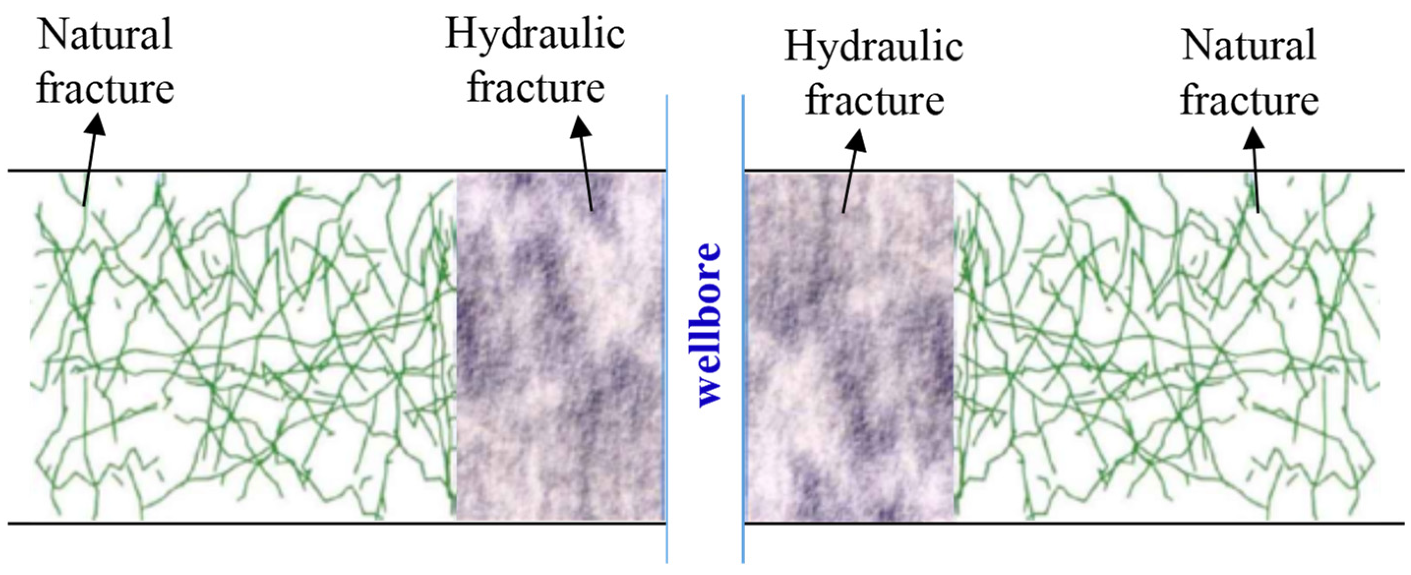
Compared with conventional naturally fractured gas reservoirs, not only is there free gas filled in the matrix pores and micro-fracture system of shale gas reservoirs, but also a large amount of natural gas is adsorbed on the rock surface of pores and fractures. Adsorbed shale gas is mainly adsorbed on the surface of matrix particles and organic matter pores, while free natural gas mainly exists in micro-fractures. Shale gas in the matrix first desorbes from the matrix skeleton and then diffuses into natural fractures, and the gas in natural fractures is transported to the hydraulic fracture in the form of seepage. Figure 1 shows a schematic diagram of fractured vertical well model in the shale gas reservoirs. It is assumed that the thickness of the gas reservoir is h, the hydraulic fracture is symmetrical with the wellbore, with a half-length of xF, a half-height of hF, and a width of wF, and the fracture can either completely penetrate the reservoir or be partially opened. The natural fractures with the matrix are idealized as a dual-porosity continuum. The gas well is produced at a constant rate. It is assumed that fluid only flows into the wellbore through the hydraulic fracture, and the internal flow of the hydraulic fracture is two-dimensional. Other basic assumptions are as follows: (1) the reservoir is slightly compressible and has a constant compressibility coefficient; (2) the adsorption of adsorbed gas follows the Langmuir isothermal adsorption law; (3) the diffusion in matrix blocks follows the Fick’s diffusion law; (4) the permeability of natural fractures is constant and horizontally isotropic; (5) the isothermal Darcy seepage occurs in natural fractures and hydraulic fracture; and (6) the effects of wellbore storage and skin effects are considered, and the influence of gravity is ignored. It is well known that both reservoir and fracture permeability values are a strong function of pressure and effective stress. However, it is difficult to handle the combined effect of the pressure-dependent permeability of the reservoir and the fracture with the proposed model. We will continue to study the influence of the pressure-dependent permeability of the reservoir and the fracture on the pressure response in detail in the following study.
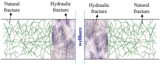
Figure 1.
Schematic of a fractured vertical well in shale gas reservoirs.
2.2. Mathematical Model
Based on the physical model established in Section 2.1, the flow of shale gas from the reservoir to the wellbore can be divided into two parts: flow in the matrix-natural micro-fractures and flow in the hydraulic fracture. The Laplace space point source function is used to establish an analytical solution for the flow in the matrix-natural micro-fractures, while the flow in the hydraulic fracture is numerically solved by the finite difference method. Finally, the flow in the reservoir and in the fractures are coupled and solved based on the continuity conditions of pressure and flow rate on the fracture surface.
2.2.1. Fluid Flow in the Hydraulic Fracture
The expression of the gas seepage–diffusion equation can be simplified by introducing generalized pseudo-pressure and pseudo-time [27]:
where p is the formation pressure, MPa; is the average formation pressure, MPa; is the pseudo-pressure of the formation, MPa2/(mPa·s); is the gas viscosity, mPa·s; Z is the deviation factor; t is the time, d; and ta is the pseudo-time, d.
In this paper, the three-dimensional distribution of the hydraulic fracture is considered, and the flow inside the fracture is no longer limited to one-dimensional flow as assumed in the conventional model. The flow equation in a finite-conductivity fracture is as follows [28]:
Assuming that at the initial moment, the pressure in the fracture is equal to the pressure in the reservoir, the initial condition is as follows:
Assuming the end of the fracture is closed, the corresponding boundary conditions are as follows:
The inner boundary condition for constant-rate production is as follows [28]:
where mi is the pseudo-pressure of the formation at the initial condition, MPa2/(mPa·s); mF is the pseudo-pressure in the hydraulic fracture, MPa2/(mPa·s); mW is the pseudo-pressure in the wellbore, MPa2/(mPa·s); is the porosity in the hydraulic fracture; ctF is the comprehensive compressibility in the hydraulic fracture, MPa−1; β1 is the conversion coefficient; wF is the fracture width, m; is the half-length of the fracture panel, m; is the half-height of the fracture panel, m; is a source term representing the gas flux entering the fracture from the matrix at a point on the fracture surface per unit volume at standard conditions, 1/d; is the gas production rate per unit volume at standard conditions, m3/d; req is the equivalent radius, m; rw is the radius of the wellbore, m; and ε, ξ is the direction of the hydraulic fracture.
Equations (1)–(8) constitute the mathematical model for fluid flow in the hydraulic fracture.
2.2.2. Fluid Flow in the Shale Gas Reservoir
The differential equation for shale gas flow in natural fractures can be expressed by the following [29]:
where mf is the pseudo-pressure in the micro-fractures, MPa2/(mPa·s); kf is the permeability of the micro-fractures, mD; kM is the general apparent permeability of the shale matrix, mD; is the porosity of the micro-fractures; ctfi is the comprehensive compressibility in the natural fractures, MPa−1; is the center position of the plane source; δ() is delta function, and often used to describe pulse signals or idealized point sources; and is a point source influx from the matrix to the micro-fractures.
In this paper, the general apparent permeability (kM) is employed to characterize the flow capacity of gas in the shale matrix [30,31]. The flow equation in the shale matrix is written as follows [32]:
Shale gas adsorption follows the Langmuir isotherm principle [32]:
Shale gas diffuses in the matrix system obeying the Fick’s diffusion law. The diffusion equation of shale gas is given by the following [32]:
The initial adsorption amount is as follows:
where α is the shape factor of the matrix, 1/m2; D is the diffusion coefficient, m2/h; VE is the equilibrium adsorption concentration, m3/m3; VEi is the equilibrium adsorption concentration at the initial condition, m3/m3; VL is the Langmuir volume, m3/m3; pL is the Langmuir pressure, MPa; mL is the Langmuir pseudo-pressure, MPa/(mPa·s).
2.3. Solution to Mathematical Model
2.3.1. Dimensionless Mathematical Model
In order to standardize and simplify the mathematical model and make the solution and result discussion of the model more general, dimensional variables are introduced to simplify the above seepage mathematical model. The dimensional parameters are shown in Table 1.

Table 1.
Input parameters for model validation.
Substituting the dimensionless parameters into Equations (1)–(8), the dimensionless differential equations of the hydraulic fracture can be obtained and expressed as follows:
The boundary conditions are as follows:
Substituting the dimensionless parameters into Equations (9)–(13), one can obtain the dimensionless differential equations of the shale reservoir.
For the micro-fracture,
The initial condition:
Outer boundary conditions:
For the matrix,
The dimensionless pseudo-steady state diffusion equation is as follows:
The model of isotherm adsorption accords with the Langmuir equation, which can be expressed as follows:
The initial amount of adsorption is as follows:
2.3.2. Solution of the Numerical Fracture Flow Model
In this section, the Laplace transformation is employed to derive the solution of the numerical fracture flow model, and the Laplace transformation equation is given by the following [33]:
where u is the Laplace transform variable.
Substituting Equations (29) and (30) into Equations (14)–(18), the dimensionless differential equations and boundaries of the hydraulic fracture in the Laplace domain are written as follows:
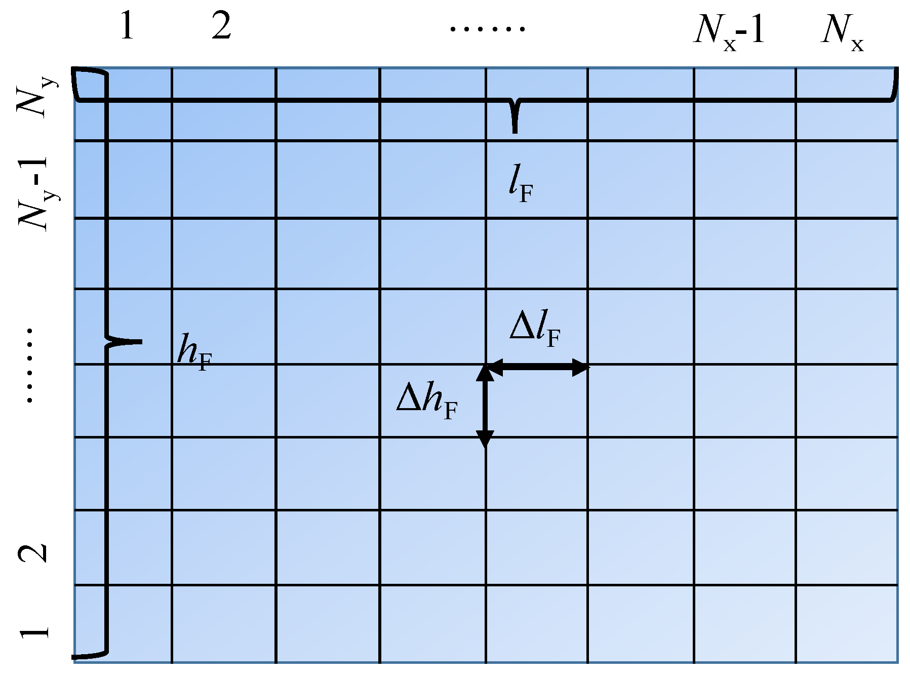
Here, we used a fracture panel shown in Figure 2 as an example to illustrate the derivation of Equation (31). The equation of the finite difference method for the fracture panel (i,j) is derived and expressed by the following:
where is the dimensionless conductivity between two neighboring fracture panels and is defined as follows:
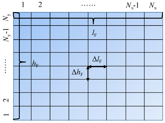
Figure 2.
Discrete hydraulic fracture along both the horizontal axis and the vertical axis.
In Equation (37), is the dimensionless conductivity between the center of the fracture panel and the adjacent grid interface, and calculated by the following:
The dimensionless conductivity between the fracture panel and the production well is given as follows:
According to Equations (36) and (40), the equations of the finite difference method for all fracture panels can be derived and written in the following matrix form:
where is the coefficient matrix; is identity matrix; is the dimensionless pressure vector of the fracture panels; is the dimensionless rate vector of the matrix to the fracture panels; is the dimensionless bottom-hole pressure; is constant vector; and is zero vector.
The production condition is given as follows:
2.3.3. Solution of the Reservoir Flow Model
Substituting Equations (29) and (30) into Equations (19)–(28), the dimensionless differential equations of the reservoir in the Laplace domain are written as follows:
Equation (44) can be rewritten as follows:
Substituting Equation (46) into Equation (43), one can obtain the following:
Based on the previous effort of research [34], the solution of point source function in three-dimensional space is derived, and the solution of Equation (47) is expressed as follows:
where
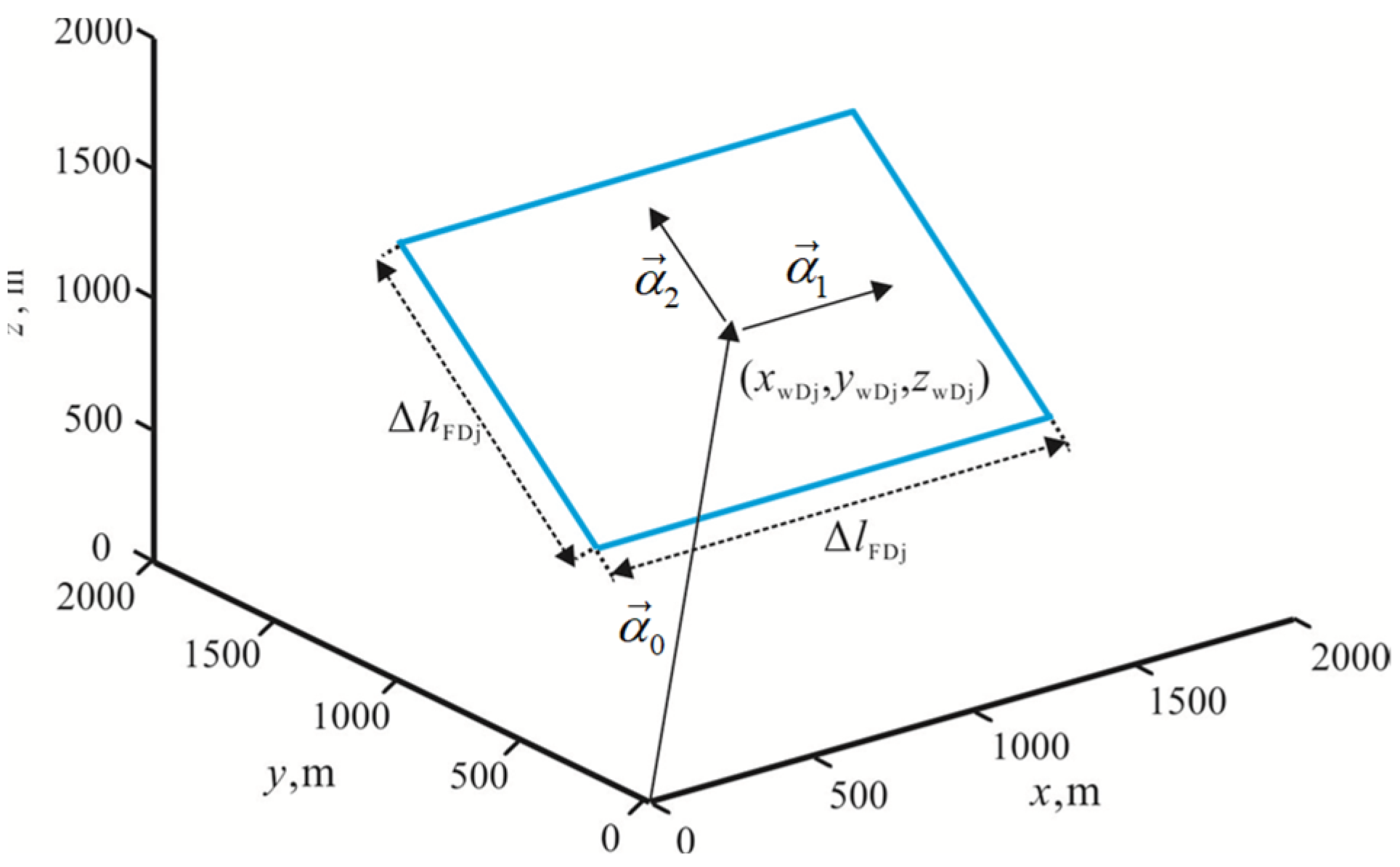
The basic parameters of the fracture panel are shown in Figure 3. The solution of plane source function can be obtained by integral Equation (49).
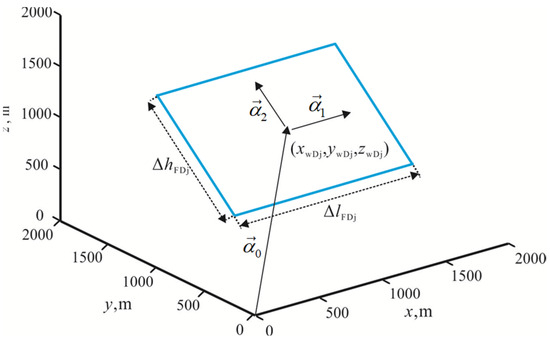
Figure 3.
Basic parameters of the fracture panels, where is the coordinate of the center of the fracture panel; is the length of the fracture panel; and is the height of the fracture panel.
With the superposition principle, for the system in Figure 3, the pressure drop at the point caused by all fracture panels can be calculated, and the equation is given by the following [28]:
According to Equation (55), the pressure response of all fracture panels can be obtained and written in the following matrix forms:
2.3.4. Coupling Conditions for Flow in the Two Systems
Coupling the solution of the numerical fracture model with the reservoir flow model, one can obtain the matrix equations of the system:
Based on the flux exchange of the two systems and the pressure continuity conditions of the fracture surface, the gas pressure continuity condition can be expressed as follows:
Solving Equation (59) yields the dimensionless pressure, the dimensionless production rate, and the dimensionless bottom-hole pressure for all fracture elements in the Laplace space. Combined with Equation (55), the dimensionless pressure at any point in the reservoir can be obtained. If wellbore storage and skin effects need to be considered, the Duhamel principle relationship can be used [34], and the Stehfest numerical algorithm can be used for numerical inversion [35]. This yields the pressure and production rate solutions in real space. By programming and plotting the relationship between the dimensionless pressure and the dimensionless pressure derivative, the dimensionless pressure and dimensionless pressure derivative curves can be obtained.
where S is the skin factor, and CD is the dimensionless wellbore storage coefficient.
3. Results and Discussion
3.1. Model Verification
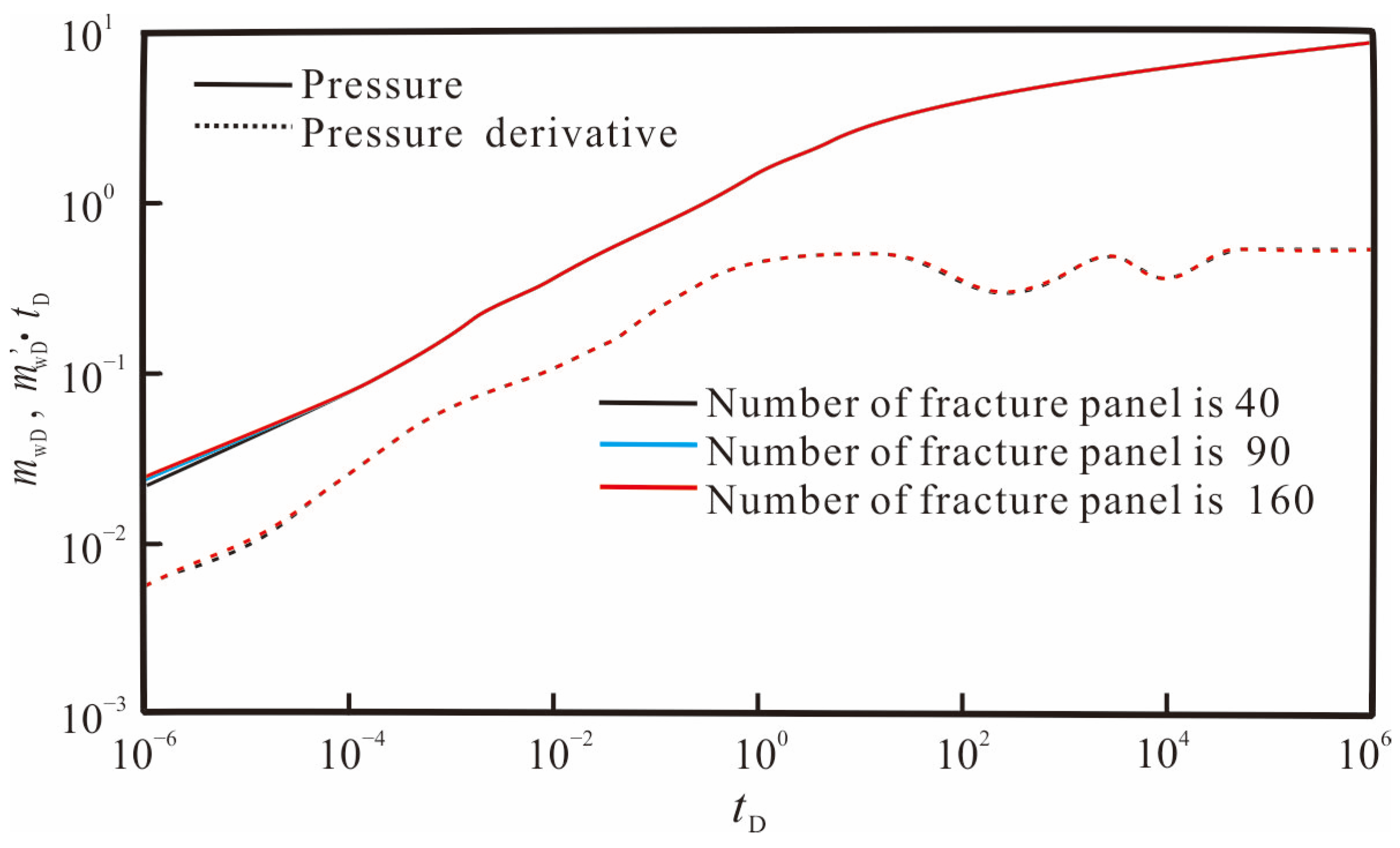
Before validating the model presented in this paper, the influence of the number of discretized fracture grids on the theoretical curve was analyzed. The hydraulic fracture is discretized into 40, 90, and 160 fracture panels, and the reservoir and fracture input parameters are shown in Table 2. Figure 4 shows the pressure dynamic response curves under different number of fracture panels. It can be seen that when the number of discretized fracture panels is greater than 90, the changes in the pressure and pressure derivative curves are very small, and the influence can be ignored. Therefore, dividing the discrete fracture into no less than 90 panels can obtain sufficiently accurate results.
Table 2.
Parameters of reservoir and fracture used for the proposed model.
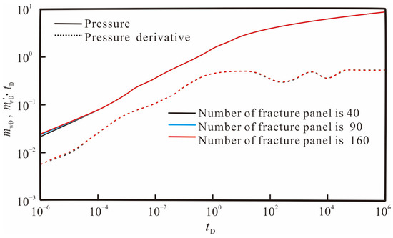
Figure 4.
Effect of the number of fracture panels on pressure and pressure derivative curves.
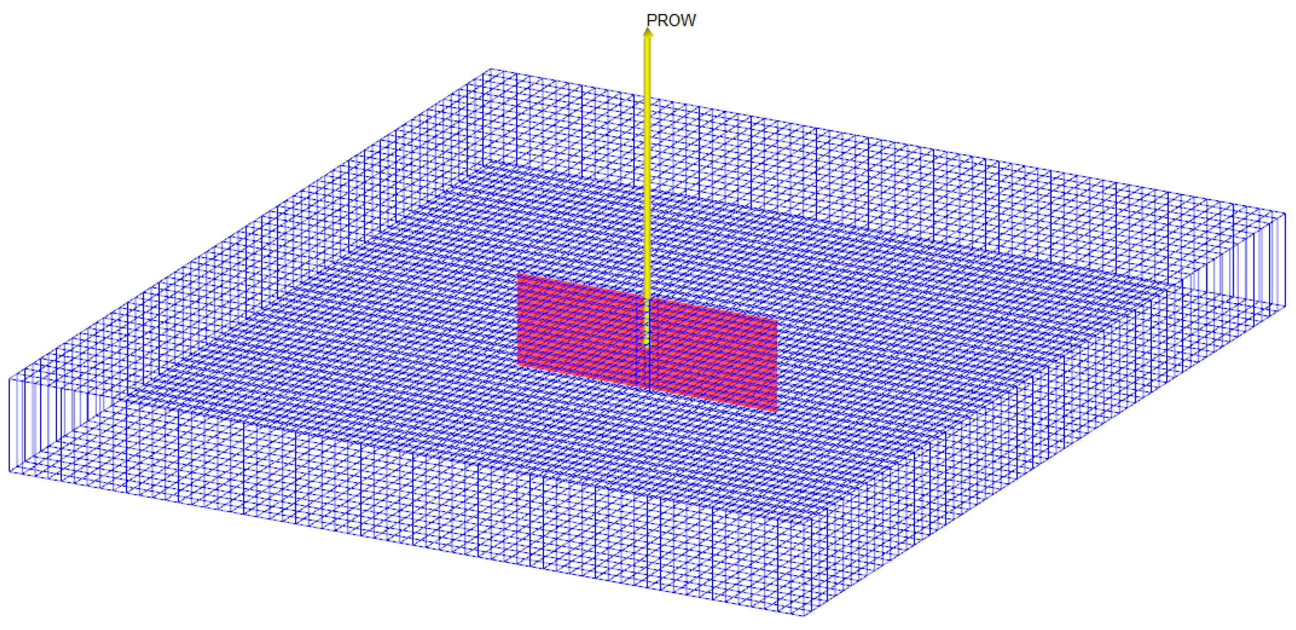
To validate the accuracy of the proposed model, a comparison is made with the commercial numerical simulation software, Eclipse (2023-09). Since most of the commercial numerical simulation software are currently used to simulate the case of three-dimensional vertical (or horizontal) fractures, it is necessary to weaken the physical model of this paper and establish a three-dimensional vertical fracture model to verify the accuracy of the research model. Firstly, a three-dimensional vertical fracture model is established using the commercial numerical simulation software, Eclipse, as shown in Figure 5. The reservoir and fracture parameters used in this case study are shown in Table 3.
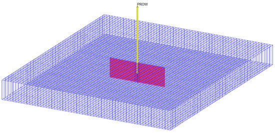
Figure 5.
Schematic diagram of fracture distribution and discretization for numerical simulation.
Table 3.
Input parameters for model verification.
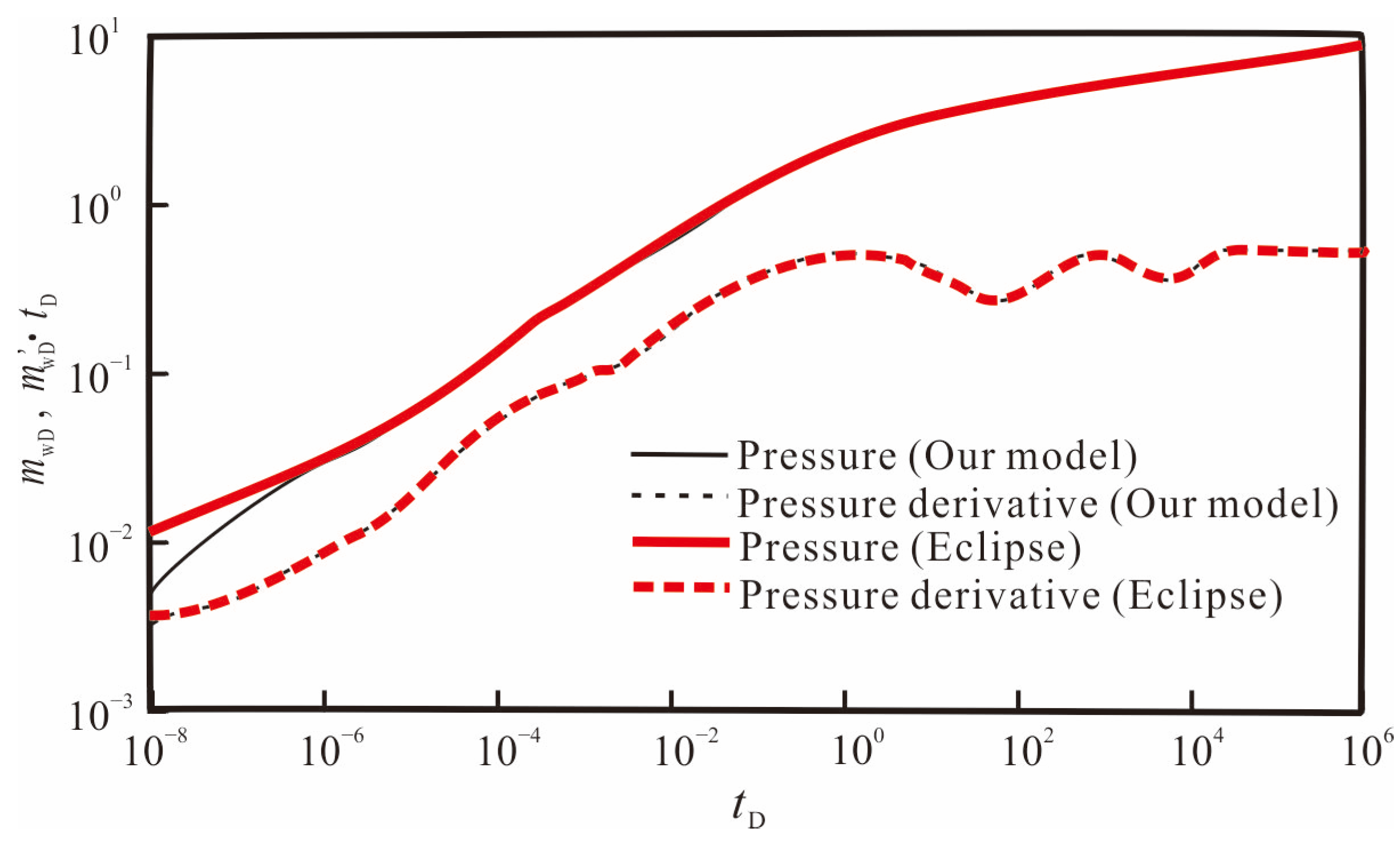
The dimensionless pressure and pressure derivative curves obtained from the model and the numerical simulation method are compared in Figure 6. It can be found that, except for the early stage of the pressure curve, which has some deviation, the curve shapes are consistent in other flow stages. The early-stage pressure deviation is mainly caused by the radial convergence effect of cracks towards the wellbore. Numerical simulation methods usually use well models to simulate early radial flow. In this study, the model introduces the confluence skin factor to correct the bottom-hole pressure and improve the accuracy of early flow simulation. Since the expression of pressure derivative has no relation to the skin, the pressure derivative curves obtained from both methods fit well throughout the entire flow stage. Currently, for numerical simulation methods, crack meshes are usually refined to obtain high-precision simulation results. After refinement, the total number of crack meshes generally reaches tens of thousands, and the simulation time step is very small, which ultimately leads to low computational efficiency and cannot meet the high-precision requirements of early crack flow in well testing interpretation analysis. The semi-analytical model established in this paper can generally characterize the crack characteristics of any distribution with few micro-elements, and the matrix system does not need to be divided into meshes. This greatly reduces the total number of meshes. In addition, the solution is not limited by the time step, so the early simulation accuracy is better, and the computational efficiency is higher. To obtain the calculation results shown in Figure 6, the new method developed in this study was used to calculate on the same platform, and the time was less than 200 s, while Eclipse’s calculation time was more than 700 s. It can be seen that the semi-analytical model studied in this paper has a significant advantage in computational efficiency.

Figure 6.
Comparison of the results between the proposed model and Eclipse.
3.2. Flow Regime Identification
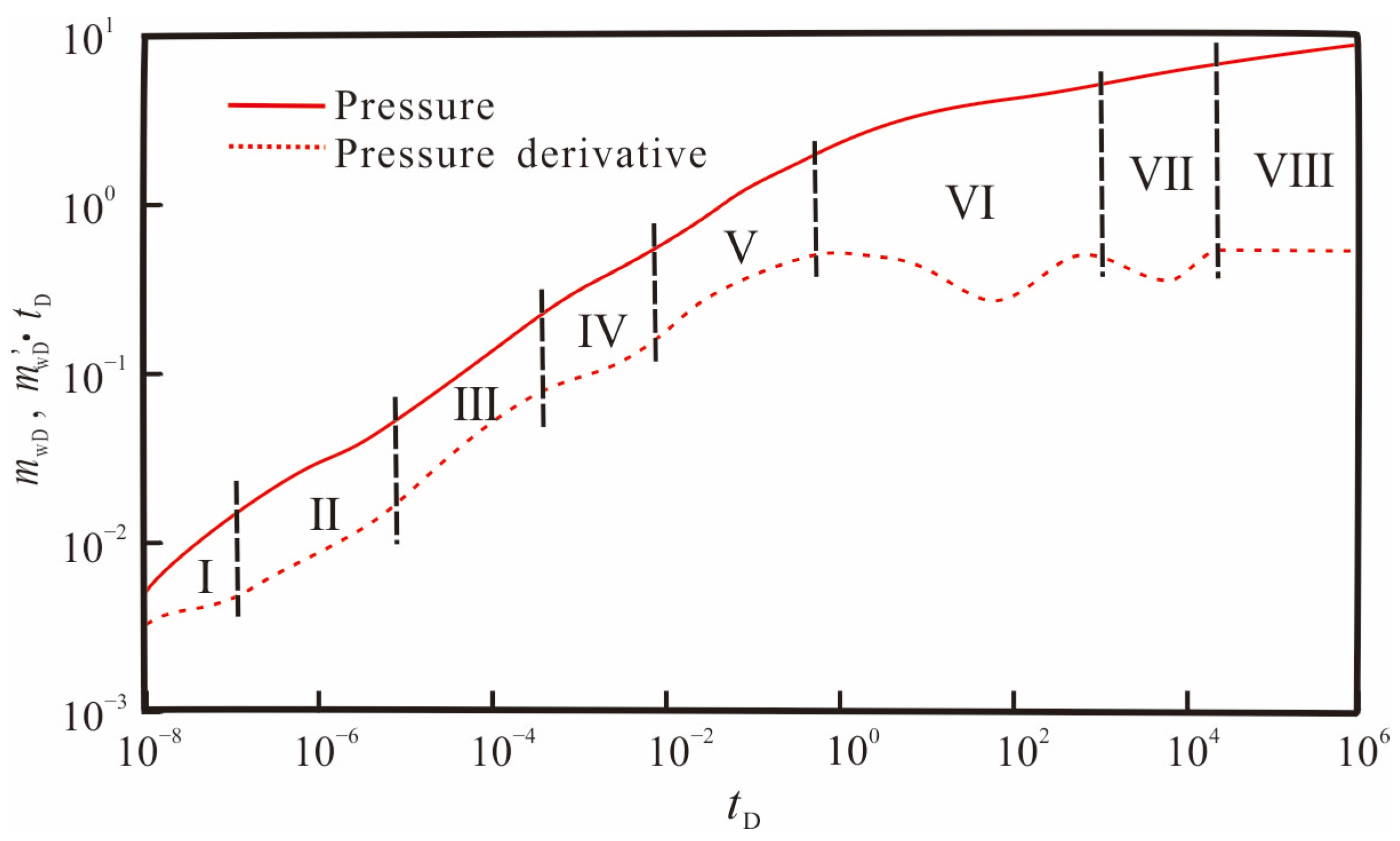
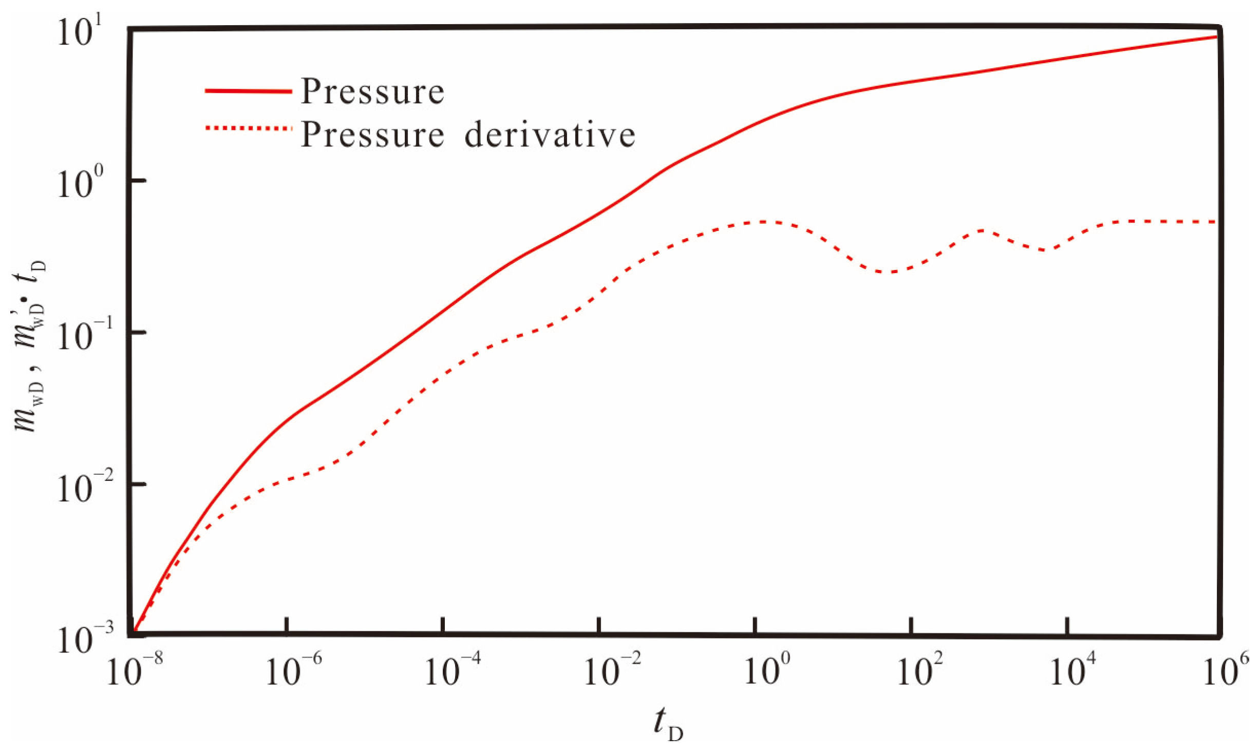
Based on the solution of the proposed model, the dynamic pressure analysis curves of shale gas wells considering the three-dimensional distribution and properties of the hydraulic fracture network is plotted, as shown in Figure 7. It can be found that eight main flow regimes can be observed from the theoretical curve:
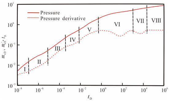
Figure 7.
The transient responses with the log–log plot.
- (1)
- First radial flow regime of the hydraulic fracture
During this period, fluid flows radially from the fracture to the wellbore, and the main characteristic of this flow stage is a horizontal line with a slope of zero on the dimensionless pseudo-pressure derivative curve.
- (2)
- Bi-linear flow regime
This regime includes linear flow from the hydraulic fracture into the wellbore and linear flow perpendicular to the fracture plane from the matrix. During this period, the pressure wave does not propagate to the top and bottom boundaries. The main feature in this flow regime is that both the dimensionless pseudo-pressure and pressure derivative curves are straight lines with a slope of 1/4.
Figure 8 shows the transient pressure dynamic curves considering the effects of wellbore storage and skin factor. It can be seen that the early radial flow and bi-linear flow stages are easily obscured with consideration of the wellbore storage effect and skin factor.
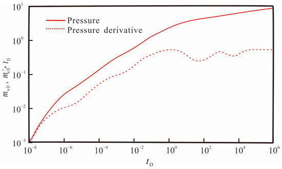
Figure 8.
The transient responses with the log–log plot considering S and CD.
- (3)
- Linear flow regime in the formation
During this flow regime, the pseudo-pressure derivative curve is a straight line with a slope of 1/2. This flow regime is mainly influenced by the dimensionless fracture conductivity and dimensionless fracture half-length and half-height.
- (4)
- The second radial flow regime
The main feature of this flow stage is a horizontal line with a slope of zero on the dimensionless pseudo-pressure derivative curve. As the pressure wave continues to propagate towards the end of the hydraulic fracture, the fluid behaves as a quasi-radial flow around the hydraulic fracture. This flow regime is mainly affected by the height of the fracture and the thickness of the reservoir. If the reservoir thickness is small or the fracture height is large, this flow stage will not appear.
- (5)
- Horizontal elliptical flow regime
This stage appears after the radial flow in the fracture, and some scholars believe that this stage is only a transitional stage between the matrix linear flow and the system radial flow. However, many scholars usually classify this flow stage as the elliptical flow stage, and the pressure derivative curve has a slope of 0.36.
- (6)
- Adsorbed gas desorption and diffusion regime
During this stage, the first “dip” can be observed on the dimensionless pseudo-pressure derivative curve, and the depth, width, and appearance time of the “dip” are mainly affected by the diffusion and seepage coefficients.
- (7)
- Inter-porosity flow from the matrix to the micro-fractures
During this stage, the second “dip” can be observed on the dimensionless pseudo-pressure derivative curve, and the depth, width, and appearance time of the “dip” are, respectively, affected by the capacitance coefficient of the micro-fracture and inter-porosity flow factor.
- (8)
- Boundary dominated flow regime
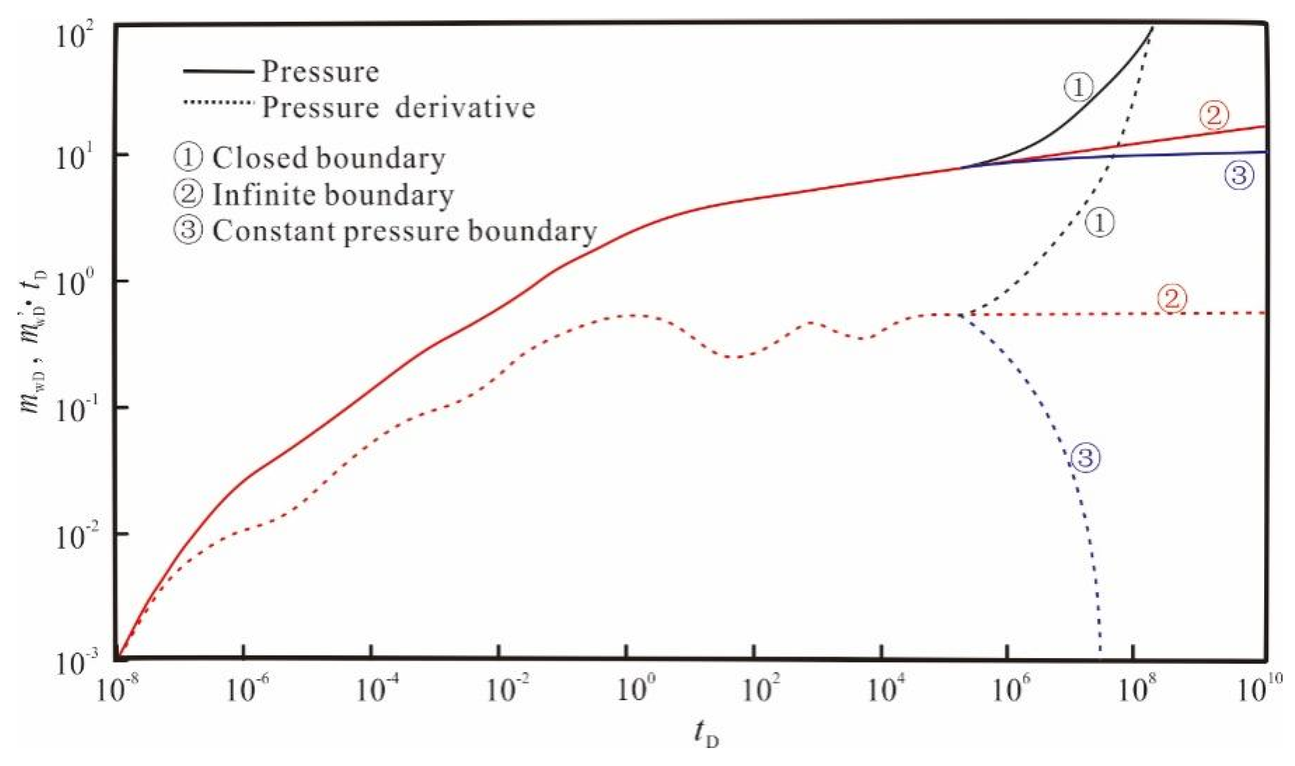
During this stage, the fluid flows radially around the hydraulic fracture, and the dimensionless pressure derivative curve is a horizontal line with a slope of 0.5. The effect of different boundary conditions on dimensionless pressure and pressure derivative curves are analyzed. It can be seen from Figure 9 that the closed boundary is represented by an upward curve of pressure and pressure derivative, and the constant pressure boundary is represented by a downward curve of pressure and pressure derivative.
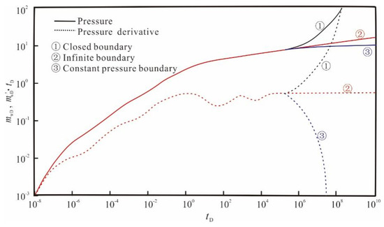
Figure 9.
The transient responses with the log–log plot considering different boundary conditions.
3.3. Sensitivity Analysis
Based on the proposed model, the effects of some key parameters on the transient pressure responses are analyzed. The basic input parameters for the model are listed in Table 3, and the range of values for each sensitive parameter is shown in Table 4.
Table 4.
Parameters used for sensitivity analysis.
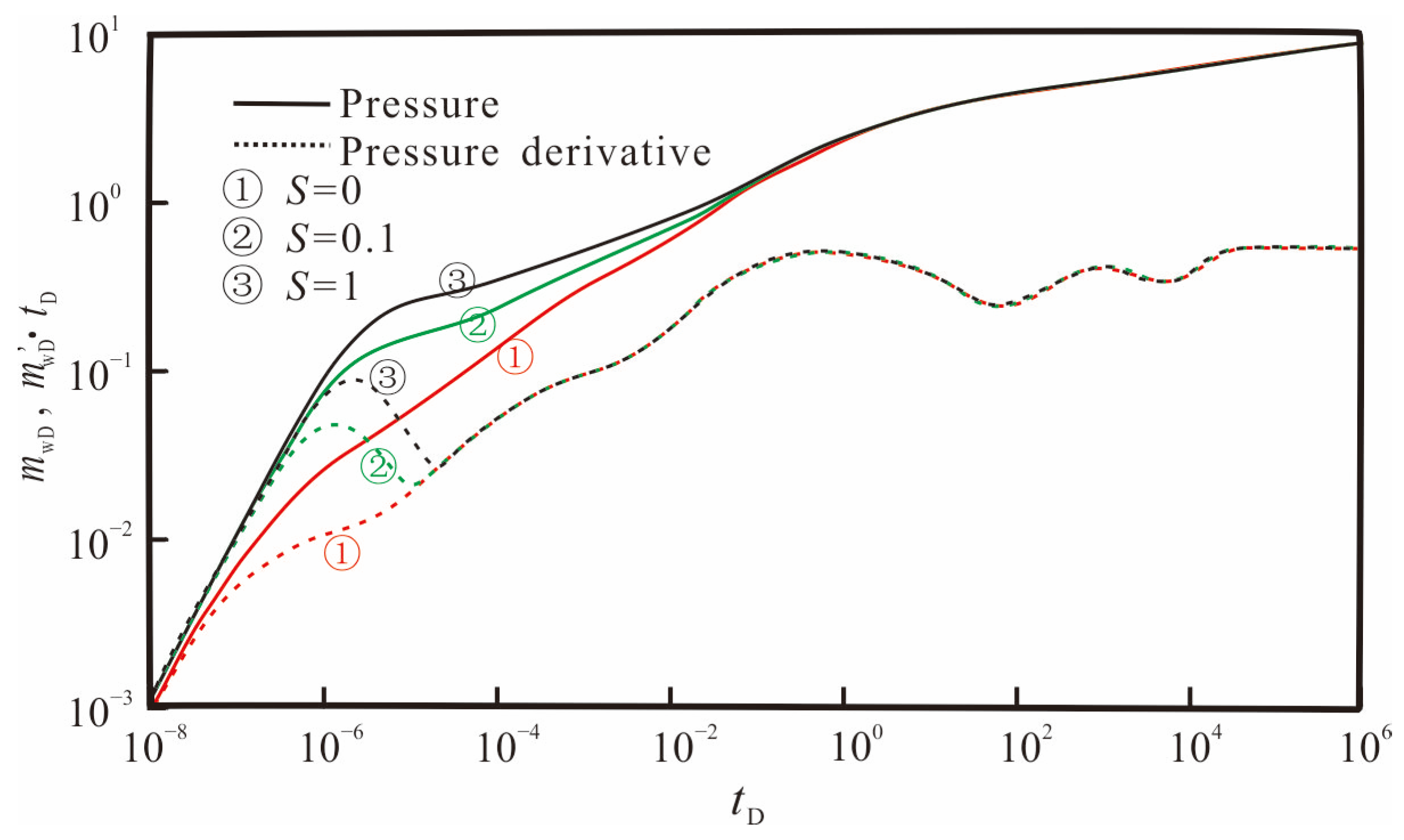
Figure 10 shows the impact of skin factors on transient pressure responses. It can be seen that as the skin factor decreases, the position of the dimensionless pressure curve becomes lower, and the position of the dimensionless pressure derivative curve “hump” becomes lower as well. This is because the smaller the skin factor, the smaller the additional pressure drop, and the faster the pressure wave propagates. Therefore, the position of the dimensionless pressure and pressure derivative curves becomes lower.
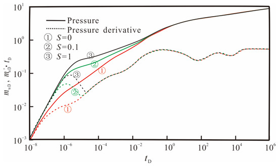
Figure 10.
Effect of skin factor on pressure and pressure derivative curves.
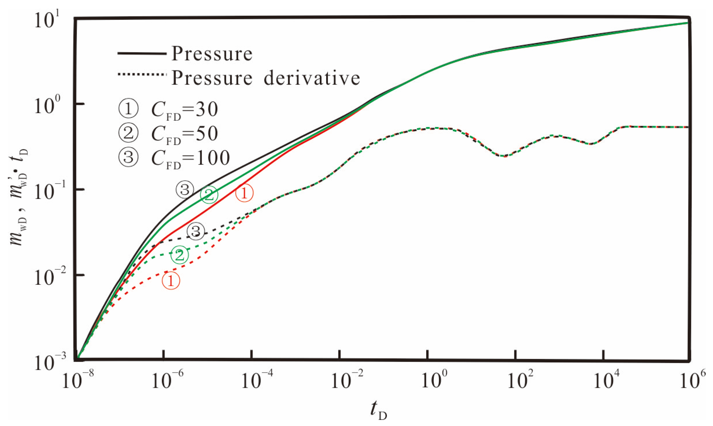
Figure 11 reflects the effect of hydraulic fracture conductivity on transient pressure responses. The dimensionless artificial fracture conductivity mainly affects the early and middle stages of the type curves. The greater the conductivity of the hydraulic fracture, the lower the position of the dimensionless pressure and pressure derivative curves. At the same time, the end time of the wellbore storage effect is earlier, and the characteristics of the fracture bi-linear flow stage are less obvious, while the duration of the linear flow in the formation is longer and more pronounced. When the conductivity increases to a certain value, the effect of the dimensionless conductivity on the type curves is not significant.
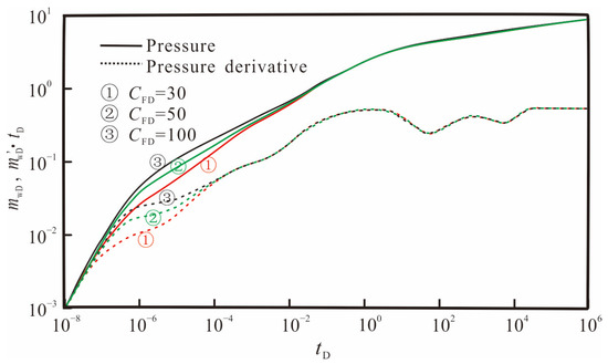
Figure 11.
Effect of fracture conductivity on pressure and pressure derivative curves.
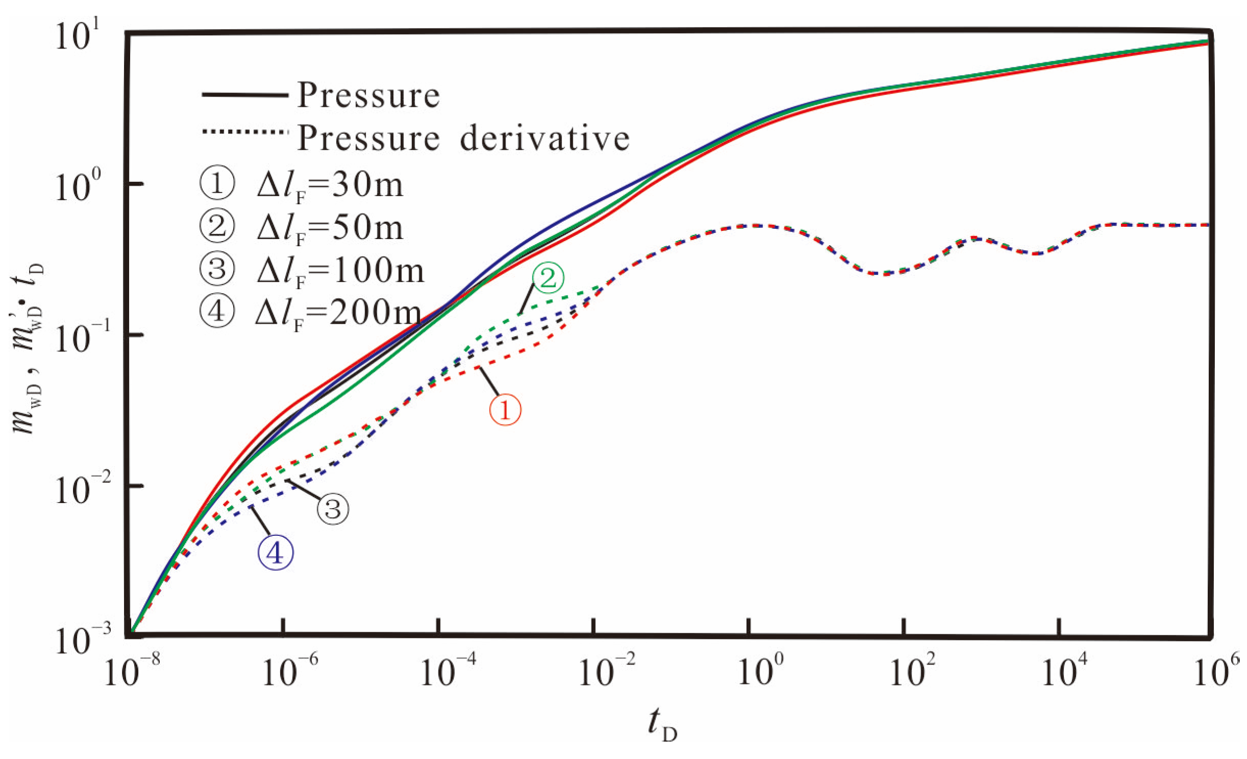
Figure 12 illustrates the impact of the half-length of the hydraulic fracture on transient pressure responses. It can be observed from the figure that as the half-length of the fracture increases, the dimensionless pseudo-pressure and pressure derivative curves move downward. This is mainly because the larger the half-length of the fracture, the larger the linear flow area of the fracture, and the smaller the pressure drop required for a given production rate. At the same time, the half-length of the fracture has a significant effect on the linear flow and radial flow stages of the fracture. The longer the half-length of the fracture, the longer the linear flow stage, and the less apparent the radial flow characteristics. If the half-length of the fracture is sufficiently large, the flow stage will transition directly from linear flow to horizontal elliptical flow.
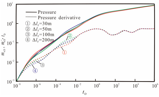
Figure 12.
Effect of fracture half-length on pressure and pressure derivative curves.
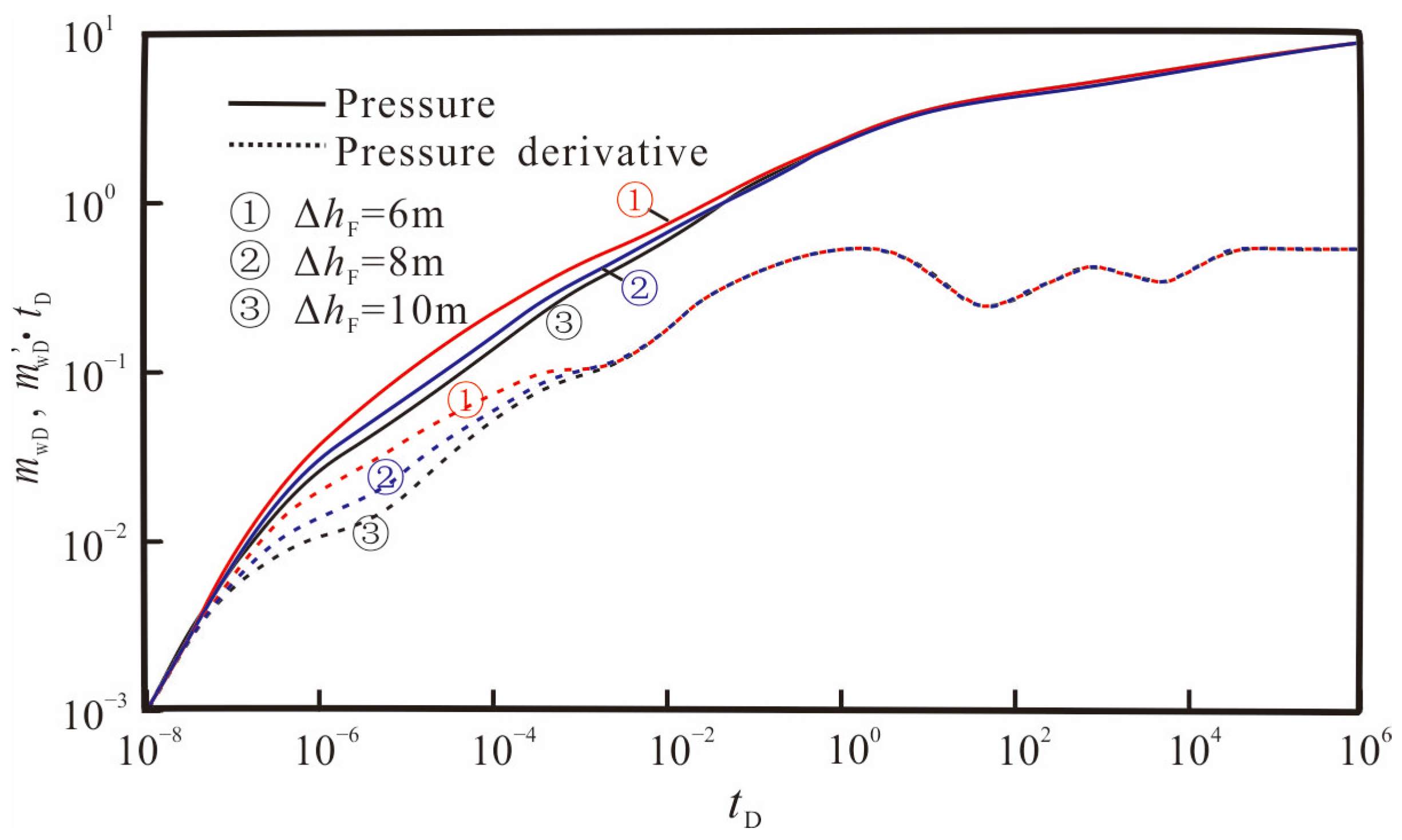
Figure 13 shows the effect of half-height of the hydraulic fracture on transient pressure responses. It can be seen from the figure that fracture height mainly affects the linear flow and radial flow stages of the fracture. At the same time, the higher the fracture height, the lower the position of the dimensionless pseudo-pressure and pressure derivative curves. This is because the larger the fracture height, the larger the contact area between the fracture and the reservoir, the smaller the flow resistance between the fracture and the gas reservoir, and the smaller the pressure drop generated.
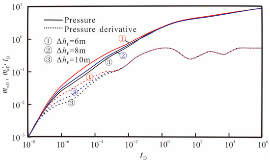
Figure 13.
Effect of fracture half-height on pressure and pressure derivative curves.
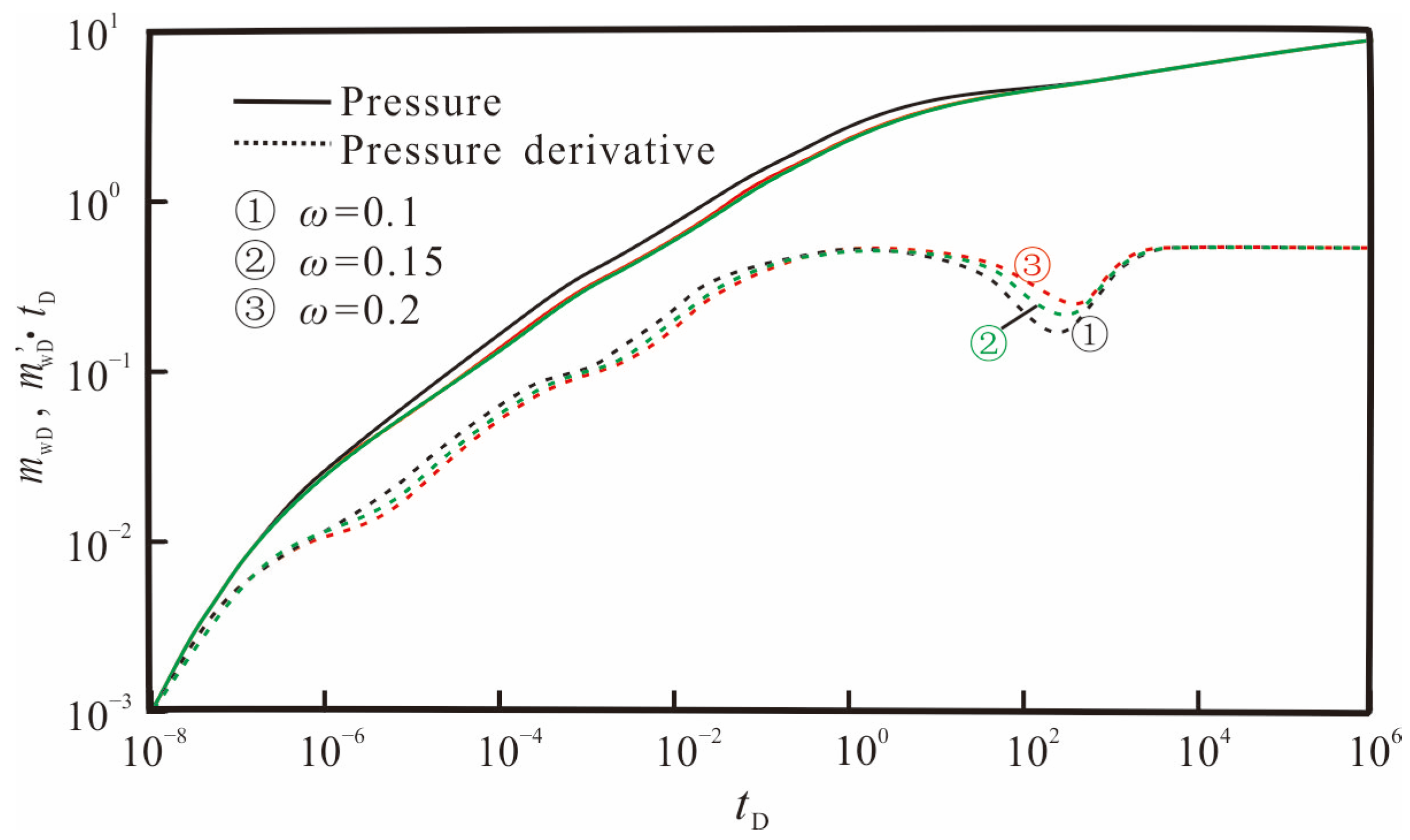
Figure 14 and Figure 15 show the influence of the storage ratio (ωf) and the inter-porosity flow factor (λMf) on transient pressure responses. From Figure 14, it can be seen that the storage ratio mainly affects the depth and width of the “dip”, with smaller ωf resulting in a wider and deeper “dip”. As defined by ωf, a smaller value indicates weaker elastic storage capacity of the micro-fracture system, relatively developed pores in the matrix system, and sufficient fluid supply to the micro-fracture system, resulting in smaller pressure drops. Conversely, a larger value of ωf indicates stronger elastic storage capacity of the micro-fracture system, poorer pore development in the matrix system, and fewer fluids in the micro-fracture system, resulting in greater pressure drops.
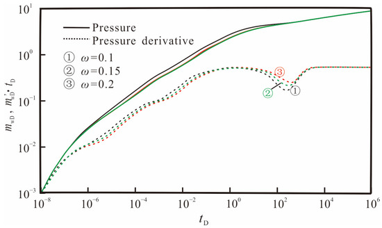
Figure 14.
Effect of the storage ratio on pressure and pressure derivative curves.
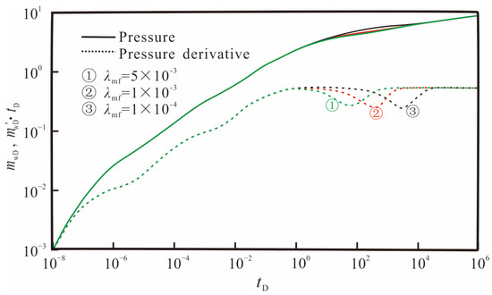
Figure 15.
Effect of inter-porosity flow factor on pressure and pressure derivative curves.
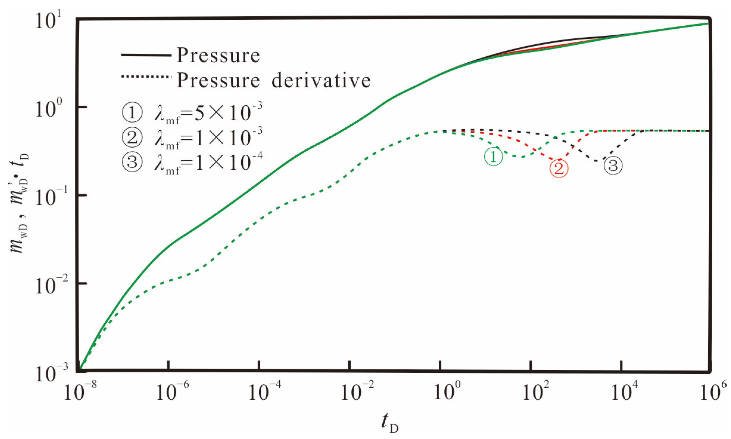
According to the definition of the inter-porosity flow factor, the smaller the ratio of matrix permeability to fracture permeability, the greater the difference in permeability between the matrix and fracture systems, and the smaller the inter-porosity flow factor. From Figure 15, it can be seen that the smaller the inter-porosity flow factor, the later the matrix-to-fracture flow occurs, and the “dip” in the dimensionless pseudo-pressure derivative curve moves to the right. The inter-porosity flow factor determines the timing of the “dip” in the pseudo-pressure derivative curve.
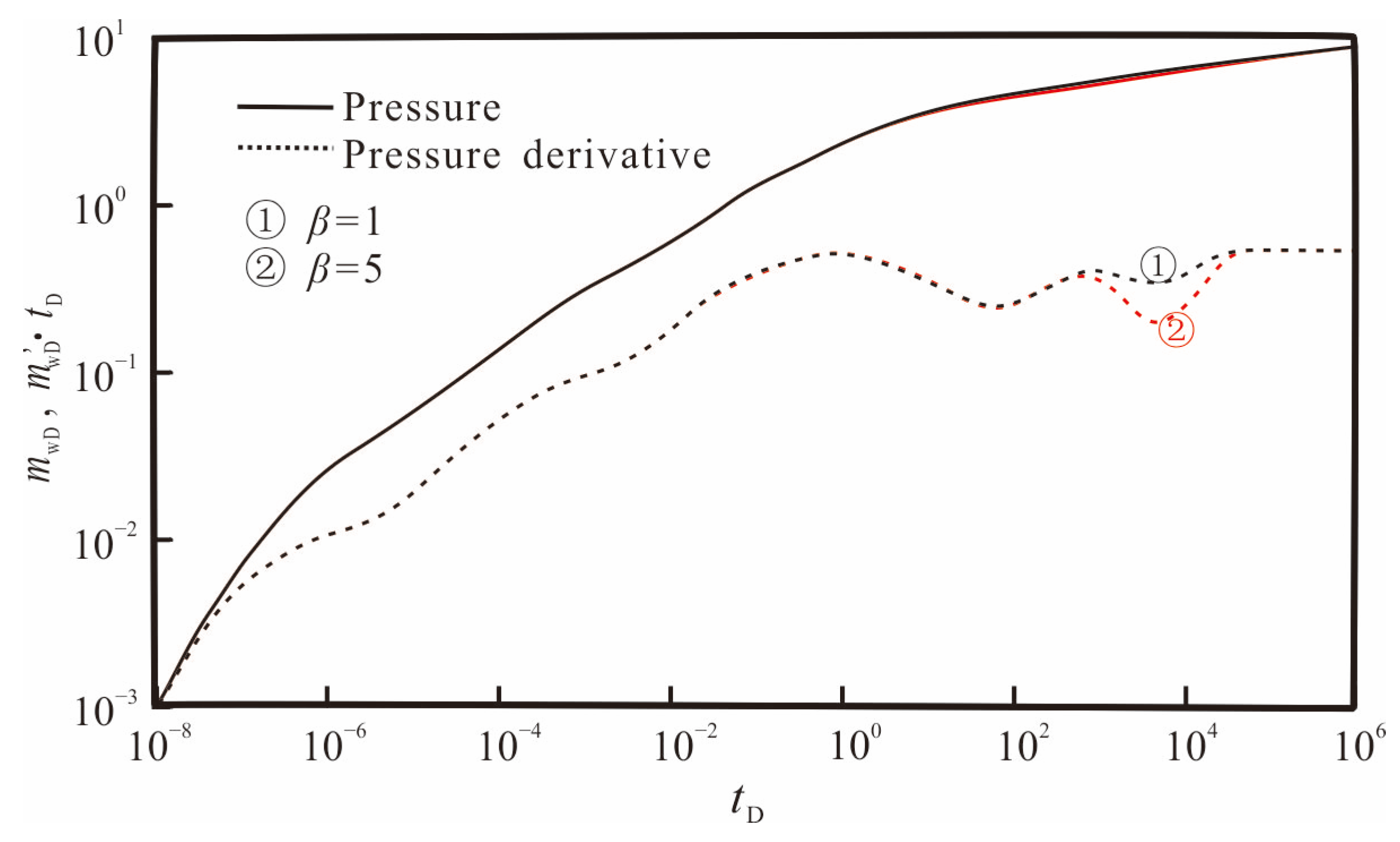
Figure 16 shows the impact of adsorption coefficient on transient pressure responses. From Figure 16, it can be seen that the adsorption coefficient mainly affects the depth and width of the “concave” section, with a larger adsorption coefficient, resulting in a wider and deeper concave section. When the adsorption coefficient is small, the “concave” sections from the matrix-fracture flow and the adsorption coefficient overlap, resulting in only one “concave” section observed on the pseudo-pressure derivative curve. This “concave” section is the result of the combined effect of two types of flow, so the width and depth of the “concave” section increase. Only when the diffusion–dispersion coefficient is larger than a certain value, the timing difference between the two types of flow is significant enough to observe two “concave” sections on the pseudo-pressure derivative curve.
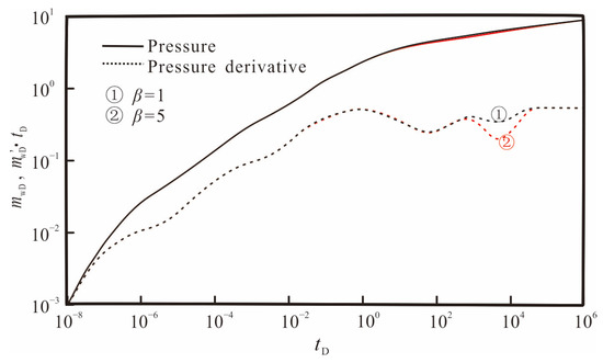
Figure 16.
Effect of adsorption coefficient on pressure and pressure derivative curves.
4. Conclusions
This paper investigates the multi-transport mechanism of shale gas within a three-dimensional fracture network and presents a novel interpretation model for testing the three-dimensional fracturing network of shale gas wells. The proposed approach utilizes a combination of the three-dimensional source function theory and the finite difference method to enable the rapid and accurate solution of the seepage model, revealing the dynamic pressure response law and clarifying the influence of key parameters of reservoir and fracturing network on the type curves. The main conclusions drawn from this research are as follows:
- The semi-analytical model employs only a small number of grid divisions for the fracture network, thereby reducing the number of grids required while allowing for a flexible description of the three-dimensional fracture distribution, leading to significant improvements in calculation efficiency. Additionally, the coupling solution method of the three-dimensional discrete fracture flow numerical solution and the reservoir flow analytical solution enhances the accuracy of the early flow simulation;
- The shale gas well testing interpretation curve obtained in this research comprises nine main flow stages: early wellbore storage and skin effect stage, first radial flow stage of fracture, bilinear flow stage, formation linear flow stage, second radial flow stage of fracture, horizontal elliptical flow stage, adsorption gas diffusion and seepage stage, inter-porosity flow stage, and outer boundary reaction stage;
- Unlike conventional gas reservoirs, shale gas reservoirs incorporate adsorbed gas. Consequently, when the pressure wave propagates to the formation, the pressure drop of shale gas reservoirs is lower than that of conventional gas reservoirs due to the replenishment of desorbed gas. The conventional gas reservoir exhibits a curve position higher than that of the shale gas reservoir on the pseudo-pressure and pseudo-pressure derivative curves;
- Under certain reservoir conditions, the artificial fracture flow capacity, fracture length, and height are the main engineering factors affecting the pressure responses of shale gas wells. The larger the fracture flow capacity, fracture length, and height, the smaller the flow resistance of shale gas, and the smaller the production pressure difference under the same production rate. Therefore, maximizing the degree and scope of reconstruction can enhance the gas well production capacity during fracturing construction.
Author Contributions
Methodology, W.G. and B.L.; Software, L.K.; Validation, G.W.; Formal analysis, X.Z. and R.Y.; Investigation, P.J., J.G., D.L. and Y.S.; Resources, Y.L. All authors have read and agreed to the published version of the manuscript.
Funding
This research received no external funding.
Data Availability Statement
Data are contained within the article.
Conflicts of Interest
Lixia Kang, Gaocheng Wang, Xiaowei Zhang, Wei Guo, Pei Jiang, Yuyang Liu, Jinliang Gao, Dan Liu, Rongze Yu, Yuping Sun were employed by PetroChina Research Institute of Petroleum Exploration and Development. The remaining authors declare that the research was conducted in the absence of any commercial or financial relationships that could be construed as a potential conflict of interest.
References
- Cao, P.; Liu, J.; Leong, Y.-K. A fully coupled multiscale shale deformation-gas transport model for the evaluation of shale gas extraction. Fuel 2016, 178, 103–117. [Google Scholar] [CrossRef]
- Wang, H.; Chen, L.; Qu, Z.; Yin, Y.; Kang, Q.; Yu, B.; Tao, W.-Q. Modeling of multi-scale transport phenomena in shale gas production—A critical review. Appl. Energy 2020, 262, 114575. [Google Scholar] [CrossRef]
- Zhao, Y.; Zhang, L.; Xiong, Y.; Zhou, Y.; Liu, Q.; Chen, D. Pressure response and production performance for multi-fractured horizontal wells with complex seepage mechanism in box-shaped shale gas reservoir. J. Nat. Gas Sci. Eng. 2016, 32, 66–80. [Google Scholar] [CrossRef]
- Zhao, X.; Rui, Z.; Liao, X.; Zhang, R. A simulation method for modified isochronal well testing to determine shale gas well productivity. J. Nat. Gas Sci. Eng. 2015, 27, 479–485. [Google Scholar] [CrossRef]
- Huang, T.; Guo, X.; Chen, F. Modeling transient flow behavior of a multiscale triple porosity model for shale gas reservoirs. J. Nat. Gas Sci. Eng. 2015, 23, 33–46. [Google Scholar] [CrossRef]
- Wei, S.; Xia, Y.; Jin, Y.; Chen, M.; Chen, K. Quantitative study in shale gas behaviors using a coupled triple-continuum and discrete fracture model. J. Pet. Sci. Eng. 2019, 174, 49–69. [Google Scholar] [CrossRef]
- Lin, L.; Li, G.; Zhao, J.; Ren, L.; Wu, J. Productivity model of shale gas fractured horizontal well considering complex fracture morphology. J. Pet. Sci. Eng. 2022, 208, 109511. [Google Scholar]
- Zhao, Y.-L.; Zhang, L.-H.; Zhao, J.-Z.; Luo, J.-X.; Zhang, B.-N. “Triple porosity” modeling of transient well test and rate decline analysis for multi-fractured horizontal well in shale gas reservoirs. J. Pet. Sci. Eng. 2013, 110, 253–262. [Google Scholar] [CrossRef]
- Yu, W.; Xu, Y.; Liu, M.; Wu, K.; Sepehrnoori, K. Simulation of shale gas transport and production with complex fractures using embedded discrete fracture model. AIChE J. 2018, 64, 2251–2264. [Google Scholar] [CrossRef]
- Zhao, Y.; Lu, G.; Zhang, L.; Wei, Y.; Guo, J.; Chang, C. Numerical simulation of shale gas reservoirs considering discrete fracture network using a coupled multiple transport mechanisms and geomechanics model. J. Pet. Sci. Eng. 2020, 195, 107588. [Google Scholar] [CrossRef]
- Tian, L.; Xiao, C.; Liu, M.; Gu, D.; Song, G.; Cao, H.; Li, X. Well testing model for multi-fractured horizontal well for shale gas reservoirs with consideration of dual diffusion in matrix. J. Nat. Gas Sci. Eng. 2014, 21, 283–295. [Google Scholar] [CrossRef]
- Ren, J.; Guo, P. A novel semi-analytical model for finite-conductivity multiple fractured horizontal wells in shale gas reservoirs. J. Nat. Gas Sci. Eng. 2015, 24, 35–51. [Google Scholar] [CrossRef]
- Xu, Y.; Liu, X.; Hu, Z.; Duan, X.; Chang, J. Bottom-hole pressure drawdown management of fractured horizontal wells in shale gas reservoirs using a semi-analytical model. Sci. Rep. 2022, 12, 22490. [Google Scholar] [CrossRef] [PubMed]
- Wu, Y.; Cheng, L.; Huang, S.; Jia, P.; Zhang, J.; Lan, X.; Huang, H. A practical method for production data analysis from multistage fractured horizontal wells in shale gas reservoirs. Fuel 2016, 186, 821–829. [Google Scholar] [CrossRef]
- Fan, D.; Ettehadtavakkol, A. Semi-analytical modeling of shale gas flow through fractal induced fracture networks with microseismic data. Fuel 2017, 193, 444–459. [Google Scholar] [CrossRef]
- Yang, R.; Huang, Z.; Li, G.; Yu, W.; Sepehrnoori, K.; Lashgari, H.R.; Tian, S.; Song, X.; Sheng, M. A semianalytical approach to model two-phase flowback of shale-gas wells with complex-fracture-network geometries. SPE J. 2017, 22, 1808–1833. [Google Scholar] [CrossRef]
- Huang, S.; Ding, G.; Wu, Y.; Huang, H.; Lan, X.; Zhang, J. A semi-analytical model to evaluate productivity of shale gas wells with complex fracture networks. J. Nat. Gas Sci. Eng. 2018, 50, 374–383. [Google Scholar] [CrossRef]
- Xu, B.; Wu, Y.; Cheng, L.; Huang, S.; Bai, Y.; Chen, L.; Liu, Y.; Yang, Y.; Yang, L. Uncertainty quantification in production forecast for shale gas well using a semi-analytical model. J. Pet. Explor. Prod. Technol. 2019, 9, 1963–1970. [Google Scholar] [CrossRef]
- Fang, B.; Hu, J.; Xu, J.; Zhang, Y. A semi-analytical model for horizontal-well productivity in shale gas reservoirs: Coupling of multi-scale seepage and matrix shrinkage. J. Pet. Sci. Eng. 2020, 195, 107869. [Google Scholar] [CrossRef]
- Chen, Z.; Liao, X.; Zhao, X.; Dou, X.; Zhu, L. Performance of horizontal wells with fracture networks in shale gas formation. J. Pet. Sci. Eng. 2015, 133, 646–664. [Google Scholar] [CrossRef]
- Ren, L.; Lin, R.; Zhao, J.; Rasouli, V.; Zhao, J.; Yang, H. Stimulated reservoir volume estimation for shale gas fracturing: Mechanism and modeling approach. J. Pet. Sci. Eng. 2018, 166, 290–304. [Google Scholar] [CrossRef]
- Wang, H. Discrete fracture networks modeling of shale gas production and revisit rate transient analysis in heterogeneous fractured reservoirs. J. Pet. Sci. Eng. 2018, 169, 796–812. [Google Scholar] [CrossRef]
- Wang, T.; Tian, S.; Zhang, W.; Ren, W.; Li, G. Production model of a fractured horizontal well in shale gas reservoirs. Energy Fuels 2020, 35, 493–500. [Google Scholar] [CrossRef]
- Dai, C.; Liu, H.; Wang, Y.; Li, X.; Wang, W. A simulation approach for shale gas development in China with embedded discrete fracture modeling. Mar. Pet. Geol. 2019, 100, 519–529. [Google Scholar] [CrossRef]
- Zhang, D.; Dai, Y.; Ma, X.; Zhang, L.; Zhong, B.; Wu, J.; Tao, Z. An analysis for the influences of fracture network system on multi-stage fractured horizontal well productivity in shale gas reservoirs. Energies 2018, 11, 414. [Google Scholar] [CrossRef]
- Mi, L.; Jiang, H.; Mou, S.; Li, J.; Pei, Y.; Liu, C. Numerical simulation study of shale gas reservoir with stress-dependent fracture conductivity using multiscale discrete fracture network model. Part. Sci. Technol. 2018, 36, 202–211. [Google Scholar]
- Wu, Y.; Cheng, L.; Huang, S.; Bai, Y.; Jia, P.; Wang, S.; Xu, B.; Chen, L. An approximate semianalytical method for two-phase flow analysis of liquid-rich shale gas and tight light-oil wells. J. Pet. Sci. Eng. 2019, 176, 562–572. [Google Scholar] [CrossRef]
- Wang, S.; Bai, Y.; Xu, B.; Li, Y.; Chen, L.; Dong, Z.; Li, W.; Zheng, X.; Wang, X. A hybrid model for simulating fracturing fluid flowback in tight sandstone gas wells considering a three-dimensional discrete fracture. Lithosphere 2021, 2021, 7673447. [Google Scholar] [CrossRef]
- Jia, Y.-L.; Wang, B.-C.; Nie, R.-S.; Wang, D.-L. New transient-flow modelling of a multiple-fractured horizontal well. J. Geophys. Eng. 2014, 11, 15013. [Google Scholar] [CrossRef]
- Xu, J.; Wu, K.; Yang, S.; Cao, J.; Chen, Z.; Pan, Y.; Yan, B. Real gas transport in tapered noncircular nanopores of shale rocks. AIChE J. 2017, 63, 3224–3242. [Google Scholar] [CrossRef]
- Xu, J.; Wu, K.; Li, R.; Li, Z.; Li, J.; Xu, Q.; Li, L.; Chen, Z. Nanoscale pore size distribution effects on gas production from fractal shale rocks. Fractals 2019, 27, 1950142. [Google Scholar] [CrossRef]
- Wang, S.; Li, D.; Li, W. A Semi-Analytical Model for Production Prediction of Deep CBM Wells Considering Gas-Water Two-Phase Flow. Processes 2023, 11, 3022. [Google Scholar] [CrossRef]
- Bai, Y.; Wang, S.; Xu, B.; Li, D.; Fan, W.; Wu, J.; Huang, S. Prediction Model for Tight Gas Wells with Time-Dependent Mechanism and Stress Sensitivity Effect. ACS Omega 2023, 8, 43037–43050. [Google Scholar] [CrossRef] [PubMed]
- Jia, P.; Cheng, L.; Huang, S.; Liu, H. Transient behavior of complex fracture networks. J. Pet. Sci. Eng. 2015, 132, 1–17. [Google Scholar] [CrossRef]
- Stehfest, H. Algorithm 368: Numerical inversion of Laplace transforms. Commun. ACM 1970, 13, 47–49. [Google Scholar] [CrossRef]
Disclaimer/Publisher’s Note: The statements, opinions and data contained in all publications are solely those of the individual author(s) and contributor(s) and not of MDPI and/or the editor(s). MDPI and/or the editor(s) disclaim responsibility for any injury to people or property resulting from any ideas, methods, instructions or products referred to in the content. |
© 2024 by the authors. Licensee MDPI, Basel, Switzerland. This article is an open access article distributed under the terms and conditions of the Creative Commons Attribution (CC BY) license (https://creativecommons.org/licenses/by/4.0/).