Article

Intelligent Classification of Volcanic Rocks Based on Honey Badger Optimization Algorithm Enhanced Extreme Gradient Boosting Tree Model: A Case Study of Hongche Fault Zone in Junggar Basin

1
Faculty of Petroleum, China University of Petroleum-Beijing at Karamay, Karamay 834000, China
2
Research Institute of Petroleum Exploration and Development, PetroChina, Beijing 100083, China
3
School of Information, North China University of Technology, Beijing 100144, China
4
School of Geophysics, China University of Petroleum-Beijing, Beijing 102249, China
*
Author to whom correspondence should be addressed.
Processes 2024, 12(2), 285; https://doi.org/10.3390/pr12020285
Submission received: 7 December 2023 / Revised: 8 January 2024 / Accepted: 19 January 2024 / Published: 28 January 2024

Abstract

:
Lithology identification is the fundamental work of oil and gas reservoir exploration and reservoir evaluation. The lithology of volcanic reservoirs is complex and changeable, the longitudinal lithology changes a great deal, and the log response characteristics are similar. The traditional lithology identification methods face difficulties. Therefore, it is necessary to use machine learning methods to deeply explore the corresponding relationship between the conventional log curve and lithology in order to establish a lithology identification model. In order to accurately identify the dominant lithology of volcanic rock, this paper takes the Carboniferous intermediate basic volcanic reservoir in the Hongche fault zone as the research object. Firstly, the Synthetic Minority Over-Sampling Technique–Edited Nearest Neighbours (SMOTEENN) algorithm is used to solve the problem of the uneven data-scale distribution of different dominant lithologies in the data set. Then, based on the extreme gradient boosting tree model (XGBoost), the honey badger optimization algorithm (HBA) is used to optimize the hyperparameters, and the HBA-XGBoost intelligent model is established to carry out volcanic rock lithology identification research. In order to verify the applicability and efficiency of the proposed model in volcanic reservoir lithology identification, the prediction results of six commonly used machine learning models, XGBoost, K-nearest neighbor (KNN), gradient boosting decision tree model (GBDT), adaptive boosting model (AdaBoost), support vector machine (SVM) and convolutional neural network (CNN), are compared and analyzed. The results show that the HBA-XGBoost model proposed in this paper has higher accuracy, precision, recall rate and F1-score than other models, and can be used as an effective means for the lithology identification of volcanic reservoirs.

1. Introduction

Lithology identification plays an important role in the field of oil exploration and development [1]. Precisely distinguishing formation lithology can efficiently and reasonably optimize oil and gas-rich reservoirs, clarify the space-time configuration relationship of source–reservoir–cap of oil and gas reservoirs, and provide theoretical guidance for the deployment of development wells in the development process [2]. Due to the complex structure of volcanic reservoirs, the large difference in physical properties and the rapid change of lithology in the vertical direction [3,4], the boundary of log response characteristics of different lithologies is fuzzy, and the traditional lithology identification methods face difficulties.
With the rise and development of computer technology, an increasing number of scholars are using artificial intelligence algorithms for lithology identification. Machine learning algorithms can effectively solve the issues of strong nonlinearity and information redundancy between log curves [5] to realize the efficient, accurate and continuous identification of lithology [6,7,8,9,10,11,12,13]. In addition to the application of a single model, integrated models have also achieved good results in lithology prediction. Yang et al. [14] integrated the decision tree algorithm with AdaBoost to fuse multiple base classifiers into a strong classifier, which significantly improved the poor generalization of a single model. Another Boosting ensemble algorithm, XGBoost, and the random forest algorithm have been successfully applied to volcanic rock recognition in Liaohe Basin, with high recognition accuracy [15,16,17]. Due to the strong nonlinear relationship between log curves, machine learning algorithms can easily fall into local optimal values when classifying high-latitude spatial samples. Therefore, it is necessary to adjust the model parameters to make the model break out of the local optimal value, so as to obtain the global optimal value. Yu et al. and Zhang et al. [18,19] used the grid-search method to optimize the hyperparameters in the GBDT and Stacking models, respectively. However, this method proved to be less efficient owing to the various data types and multiple hyperparameters of the machine learning model, and hence a heuristic algorithm may effectively address this issue. The genetic algorithm [20] and particle swarm optimization algorithm [21,22] can efficiently find the optimal value in the hyperparameter high-dimensional space of the model. The combination of optimization algorithm and machine learning model can effectively solve the problem of machine learning models falling into local extrema and further improve the accuracy of machine learning models for lithology identification.
At present, there is no research on the integration of the HBA algorithm and the XGBoost model for application in volcanic rock lithology identification. The XGBoost model has been slightly effective in lithology prediction [23,24]. The HBA algorithm is a swarm intelligence optimization algorithm with proven and obvious advantages in convergence speed and optimization accuracy [25,26,27]. This algorithm has not been applied to lithology identification. In this paper, the traditional log curve data are used to optimize the structure of the XGBoost model based on the HBA algorithm, so as to carry out research on the lithology identification of basic volcanic rock in the Hongche fault zone. In addition, the performance differences between XGBoost, KNN, GBDT, AdaBoost, SVM, CNN and HBA-XGBoost are analyzed and compared. After that, the HBA-XGBoost model is applied to two actual wells in the study area. The prediction results are basically consistent with the real lithology, which provides a reference for lithology interpretation in volcanic reservoirs.

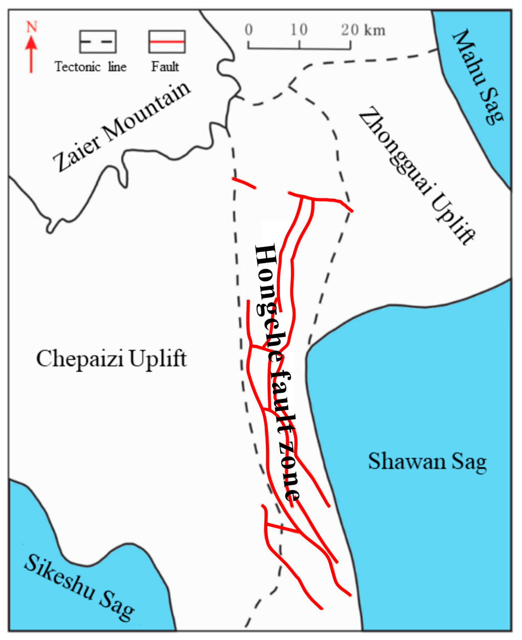
2. Geological Settings

The Hongche fault zone is located in the foreland thrust belt at the southern end of the northwestern margin of the Junggar Basin. It is generally oriented north–south [28,29]. The terrain is characterized by a high northwest and a low southeast, with a total length of about 70 km. The northern part is adjacent to the Kebai-Wuxia fault zone, the eastern part is bounded by the Zhongguai uplift and the Shawan sag and the western part is bordered by the Chepaizi uplift (Figure 1). The Carboniferous reservoir in the study area is a monoclinic structure with southeast tendency [30,31,32], which has been located in the high part of the structure for a long time. It is the oil and gas migration direction area of the Shawan sag and Sikeshu sag, and it is a favorable reservoir area for oil and gas accumulation.
The Carboniferous reservoir is an intermediate-basic volcanic reservoir with volcanic breccia, tuff rock, pyroclastic sedimentary rock, basalt, andesitic rock and sedimentary tuff [33,34], and mainly volcanic breccia in the eruptive phase [35]. The distribution of various volcanic rocks in the study area is relatively concentrated on the plane, showing a flaky distribution and poor continuity. In the vertical direction, various types of volcanic rock appear alternately. Affected by volcanic eruptions and paleotopography [36], the thickness distribution of different lithologies is uneven and the lithology is complex and changeable. These problems lead to the low accuracy of traditional lithology identification methods. Therefore, a machine learning method is urgently needed to deeply explore the relationship between log response characteristics and lithology, so as to predict volcanic lithology efficiently and accurately.

3. Principle of the HBA-XGBoost Model

3.1. Honey Badger Algorithm

The honey badger algorithm is a new intelligent optimization algorithm proposed by Hashim et al. in 2021 [37]. The honey badger algorithm imitates the group behavior of the honey badger foraging in nature to achieve the purpose of global search. The honey badger’s foraging is divided into two behaviors: digging and honey-picking. Digging behavior means that the badger uses its olfactory sense to find the approximate location of the prey, and captures the prey to complete its foraging through the digging behavior. Honey-picking behavior refers to the cooperative relationship between the honey badger and the honeyguide bird. The honey badger is not good at locating the position of beehives, but the honeyguide bird guides the honey badger directly to the beehive’s position after locating it. The honey badger destroys the beehive and both parties complete their foraging behavior.
In the honey badger algorithm, the global optimal value of the search feature space is achieved by simulating the foraging behavior of a honey badger group. Suppose that the position of the D-dimensional feature space of the ith honey badger in a honey badger population of size N is l i = [ x i 1 , x i 2 , x i 3 , , x i D ] , where i = 1 , 2 , 3 , , N .
In its digging behavior, the badger only relies on the smell of the prey to roughly locate the prey. The odor intensity of the prey is related to the density of the prey and the distance between the prey and the badger. It is expressed by the inverse square law. When the odor intensity is large, the badger will accelerate its movement speed. On the contrary, when the odor intensity is small, the badger will slow its movement speed. In order to ensure the smooth transition from locating prey to digging prey and reduce the randomization in the iterative process, a density factor α that gradually decreases with time is introduced, which is defined in Equation (1).
α = C × exp ( t t max )
where α is the density factor; tmax is the maximum number of iterations; t is the current number of iterations; and C is a constant, generally set to 2.
In the digging behavior of honey badgers, the population position is constantly updated. The location update of the digging behavior is defined in Equation (2). In this process, the search action of the badger is similar to the shape of a heart. In this process, the location update of the badger is affected by the smell I of the prey, the distance di between the badger and the prey and the density factor α. In addition, in the process of capturing prey, the badger will be disturbed by other signals, thus changing the direction of its search for prey, which makes it possible to find a better prey location. The location update of the honey-picking behavior is defined in Equation (3). During the honey-picking process, the honey badger is directly guided by the honeyguide bird to locate the honey. Similarly, the process will also be disturbed by other signals to change the search direction. With the continuous updating of the population position, the badger will capture its prey and complete its foraging behavior (i.e., find the global optimal solution).
x n e w = x p r e y + F × β × I × x p r e y + F × r 2 × α × d i × | cos ( 2 π r 3 ) × [ 1 cos ( 2 π r 4 ) ] |
x n e w = x p r e y + F × r 5 × α × d i
where xnew is the location of the honey badger after updating; xprey is the prey position, that is, the optimal position currently searched in the global space; β is a constant, generally set to 6, reflecting the ability of badgers to search for prey; di is the distance between the badger and the prey; r2, r3, r4, r5 are four different random numbers between 0 and 1 and F is the sign of changing the search direction, taking a value of 1 or −1.

3.2. XGBoost Model Principle

XGBoost is a Boosting ensemble learning model proposed by Chen. [38]. The main idea is to use the gradient boosting algorithm [39] to combine multiple weak classifiers (linear classifiers or Cart decision trees). In this paper, the Cart decision tree is used. In each iteration, by correcting the residuals of the constructed weak classifiers, a new base classifier is generated using the gradient descent algorithm, which constantly makes the objective function approach the minimum direction, and the gap between the predicted value and the real value becomes smaller, with the ultimate goal of obtaining a strong classifier. The prediction result is the addition model of all weak classifiers. The XGBoost model shows excellent results in both classification and regression problems.
The XGBoost model is further optimized based on the GBDT model. Compared with GBDT, the loss function of XGBoost is expanded by the second-order Taylor formula, which further improves the prediction accuracy. Moreover, a regular term is added on the basis of the objective function to prevent over-fitting of the tree model and increase the robustness and versatility of the model algorithm. In addition, the XGBoost model adopts a block storage structure, which can be operated in parallel when the tree is generated, which significantly improves the running speed. The objective function can be written as follows:
X o b j = j = 1 T [ ( i g i ) w j + 1 2 ( i h i + λ ) w j 2 ] + λ T
where g i = y ^ ( t 1 ) l ( y i , y ^ ( t 1 ) ) represents the first derivative of the loss function term and h i = y ^ ( t 1 ) 2 l ( y i , y ^ ( t 1 ) ) represents the second derivative of the loss function. T is the number of leaf nodes, wj is the weight of leaf nodes and γ is a penalty coefficient.
When the objective function is the smallest, the optimal solution wj* of each leaf node weight and the optimal target value Xobj* can be obtained as follows:
w j * = i g i t h i + λ X o b j * = 1 2 j = 1 T ( i g i ) 2 i h i + λ + γ T

3.3. HBA-XGBoost Model Principle

XGBoost is affected by multiple hyperparameters in solving the problem of lithology classification. Therefore, the input of non-optimal hyperparameters when constructing the XGBoost model will reduce the prediction accuracy and model generalization of the model. In order to solve this problem, the HBA algorithm is introduced to optimize the XGBoost lithology prediction model. The HBA algorithm improves the prediction accuracy and robustness of the XGBoost lithology classification model by finding the optimal parameters in the hyperparameter feature space as the input of the XGBoost model. The workflow of the HBA-XGBoost model is as described in the list below (Figure 2). The complexity of the model mainly depends on the number of iterations of the HBA algorithm, and the overall complexity is the product of the complexity of the HBA algorithm and the complexity of the XGBoost algorithm.
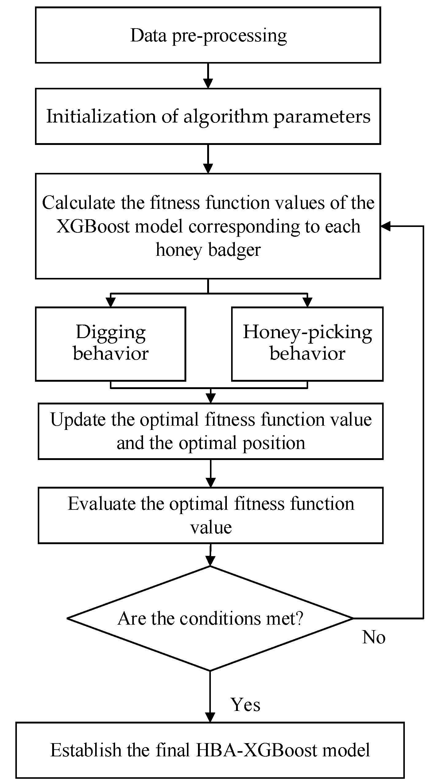
  • Data cleaning of the volcanic rock data set, missing value processing, log curve standardization, data feature selection, data set division and other pre-processing work are carried out to ensure data quality and consistency.
  • Using the honey badger optimization algorithm, the honey badger population is initialized according to the XGBoost hyperparameter feature. Each honey badger represents a combination of XGBoost hyperparameter features. Initial conditions are defined, such as density factors (α), sign to change direction (F) and the honey badger’s ability to catch prey (β).
  • The XGBoost model is used as the fitness evaluation function of the HBA model. The XGBoost model is trained according to each individual of the badger population. The model performance is evaluated by cross-validation, and the calculated performance index is passed to the HBA model.
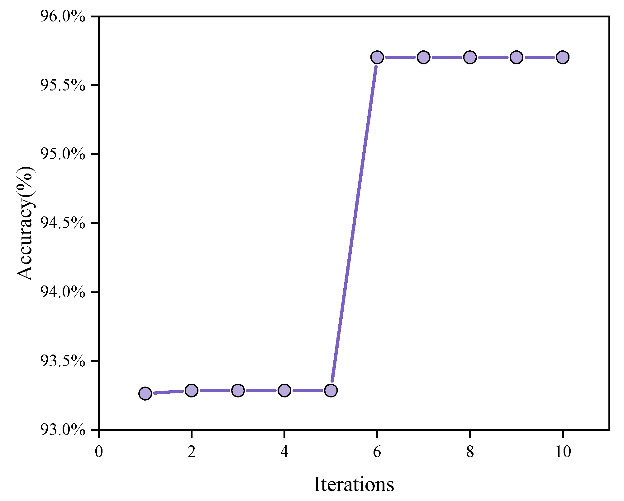
  • The HBA model uses Equations (2) and (3) to update the positions of the individuals of the badger population to complete the foraging behavior according to the badger’s two foraging strategies (digging behavior and honey-picking behavior), that is, the its seeks the best combination of hyperparameters. After the population position is updated, the fitness function is recalculated and the population positions are continuously iterated. Finally, the globally optimal individual is selected as the optimal hyperparameter combination.
  • The XGBoost model is trained with the globally optimal hyperparameter combination, and the HBA-XGBoost optimization model is obtained to evaluate and predict the lithology of volcanic rock.

3.4. Model Evaluation Index

The confusion matrix can clearly reflect the difference between the true label and the predicted label (Table 1). When the true label is positive and the predicted label is also positive, it is defined as a true positive (TP). False negative (FN), false positive (FP) and true negative (TN) are also defined in the table. According to the confusion matrix, the four indicators Accuracy, Precision, Recall and F1-score can be calculated. Accuracy reflects the prediction accuracy of the model as a whole. Precision and recall mainly reflect the prediction accuracy of the model for a certain type of lithology. F1-score is the harmonic average of precision and recall. The higher the four indicators, the better the performance of the model in the volcanic rock lithology recognition task.
A c c u r a c y = T P + T N T P + F N + F P + T N
Precision = T P T P + F P
Recall = T P T P + F N
F 1 - score = 2 × Precision × Recall Precision + Recall

4. Data Analysis and Processing

The data needed in this study are from the log and mud-log data of 38 wells in the Hongche fault zone. Every 0.125 m of log data is taken as a sample point. The target task is to complete the identification of the six lithologies pyroclastic sedimentary rock (H1), volcanic breccia (H2), sedimentary tuff (C1), tuff (N1), andesite (A1) and basalt (X1). In order to complete the task of lithology identification, this study adopts eight conventional log curves as important features of lithology identification: natural gamma curve (GR); caliper curve (CALI); spontaneous potential curve (SP); electrical curves—original formation resistivity (RT) and flushing zone formation resistivity (RXO); and physical property curves—acoustic curve (AC), density curve (DEN) and neutron curve (CNL). Table 2 shows the range of different curve values for each target lithology.
At present, the method of log curve cross plot is often used to identify lithologies [40]. The cross plot can clearly reflect the distribution of log response characteristics corresponding to different lithologies. Figure 3 shows the two-dimensional kernel density maps of all log curves intersected by lithology, and the diagonal shows the distribution of log response characteristics among different lithologies. It can be clearly seen that although the concentration degree of log response characteristics of different lithologies is slightly different, much of the data are in a mixed or superimposed state. This is due to the large amount of redundant information in the log curves. Therefore, it is not possible to identify volcanic rock lithology according to the intersection of log curves alone. It is necessary to adopt a machine learning method that can analyze multi-dimensional and multiscale data efficiently to divide the lithology characteristics.
There is an imbalance in the number of samples in the volcanic rock data set, which will lead to the loss of accuracy and universality in the created model. In this study, the SMOTEENN oversampling method [41] is used to increase the number of minority samples, improve the classification performance of the model for minority samples, and introduce a certain degree of new information to enrich the diversity of samples. The sampling results for each lithology are shown in Figure 4. The number of minority samples increased, balancing the proportion of different lithologies in the data set. At the same time, a large number of H2 lithology samples removed redundant data and reduced the over-fitting in the model training. The specific operation process is as follows (taking sedimentary tuff as an example):
  • For all samples x in the sedimentary tuff, the Euclidean distance to other samples is calculated to obtain K-nearest neighbor samples.
  • The oversampling coefficient is determined according to the proportion of sedimentary tuff and most samples. For each sample of sedimentary tuff, xi, n samples are obtained by oversampling with Equation (10) to increase the number of minority samples.
x n e w = x i + r a n d ( 0 , 1 ) * ( x i k i )
where xnew is a new sample obtained by oversampling, xi is a sedimentary tuff sample, rand(0,1) is a random number between 0 and 1 and ki is a neighbor sample.
3.
After increasing the number of samples, the redundant and repeated data samples are deleted to prevent over-fitting in subsequent training.
4.
The data set is standardized after sampling, eliminating the influence of different dimensions, increasing the operation speed and preparing for the following modeling.

5. Results

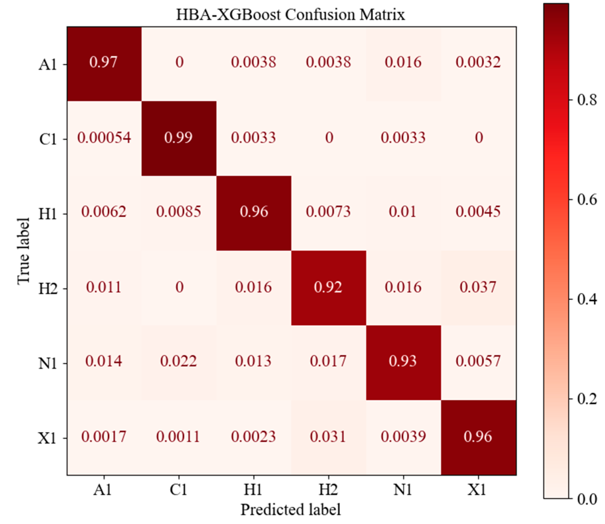
5.1. HBA-XGBoost Application Effect

The model effect of XGBoost will be affected by the input hyperparameters when constructing the model. Therefore, the HBA algorithm was used to optimize the hyperparameters. The default values and meaning of different hyperparameters are shown in Table 3. In this study, the seven hyperparameters in Table 3 were optimized at the same time. The number of badger populations in the HBA model was set to 50 and the dimension of each badger was 7, corresponding to 7 hyperparameters. The ability of badgers to capture prey was 6, and the accuracy of the XGBoost model was used as the fitness function. Figure 5 shows that the accuracy of the model was basically unchanged after 6 iterations. The accuracy of the XGBoost model was increased from the initial 93.2% to 95.7%, and the convergence speed was fast. At this time, the global optimal value was found (Table 3). The global optimal value searched for by the HBA model was used as the input of the XGBoost model to construct the HBA-XGBoost model.
The data set was divided into a training set and a test set according to the ratio 7:3, and the final accuracy of the test set was 95.70%. In Table 4, the F1-score of the HBA-XGBoost model for different lithologies was above 92%, with an average of 95.64%. The average accuracy and recall rate of different lithologies were also basically above 95%. Figure 6 is the confusion matrix predicted by the HBA-XGBoost model. The prediction accuracy of each lithology was greater than 92%, of which C1 had the highest prediction accuracy, followed by A1. In short, HBA-XGBoost had a good recognition effect in the volcanic rock classification task.

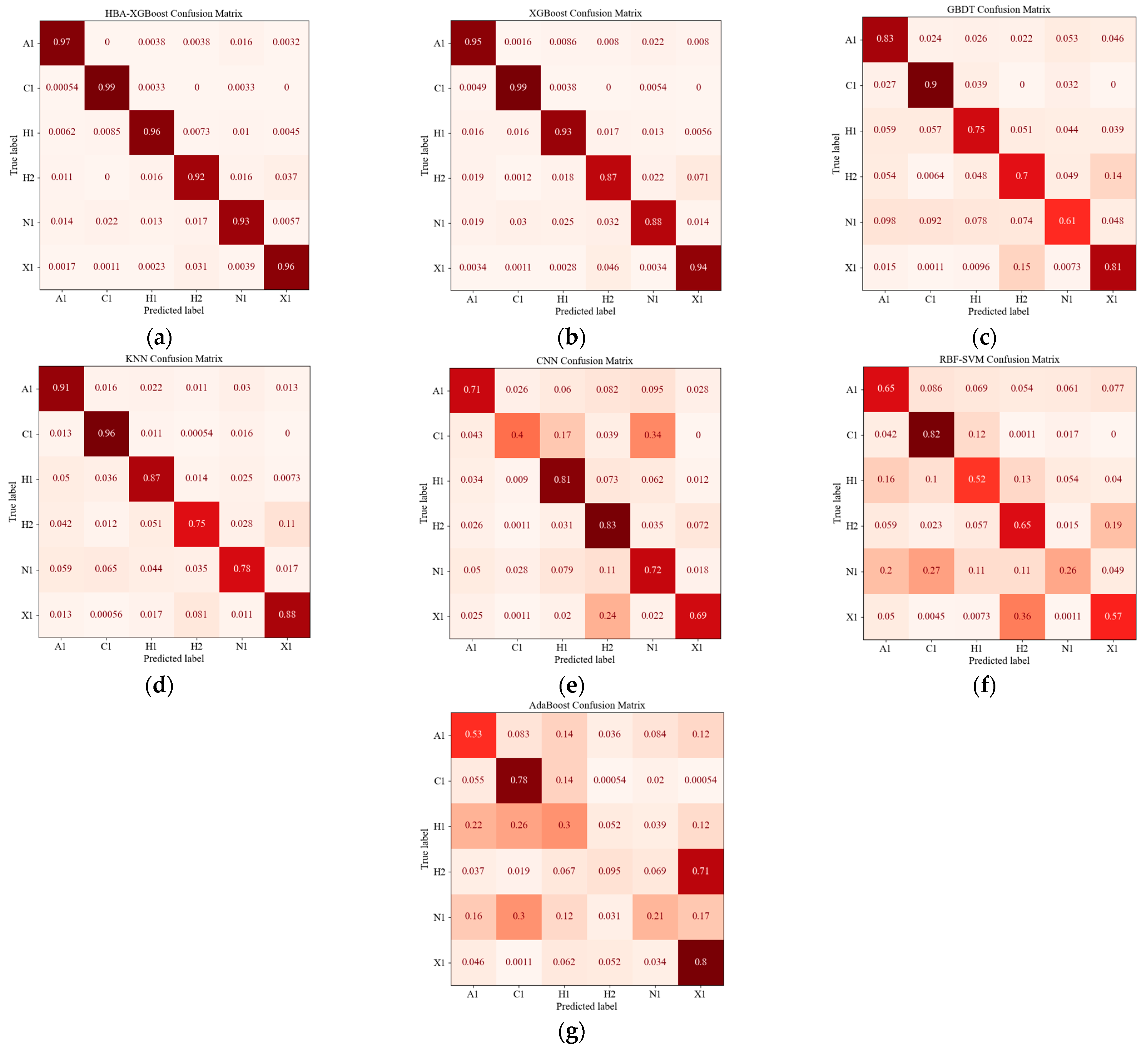
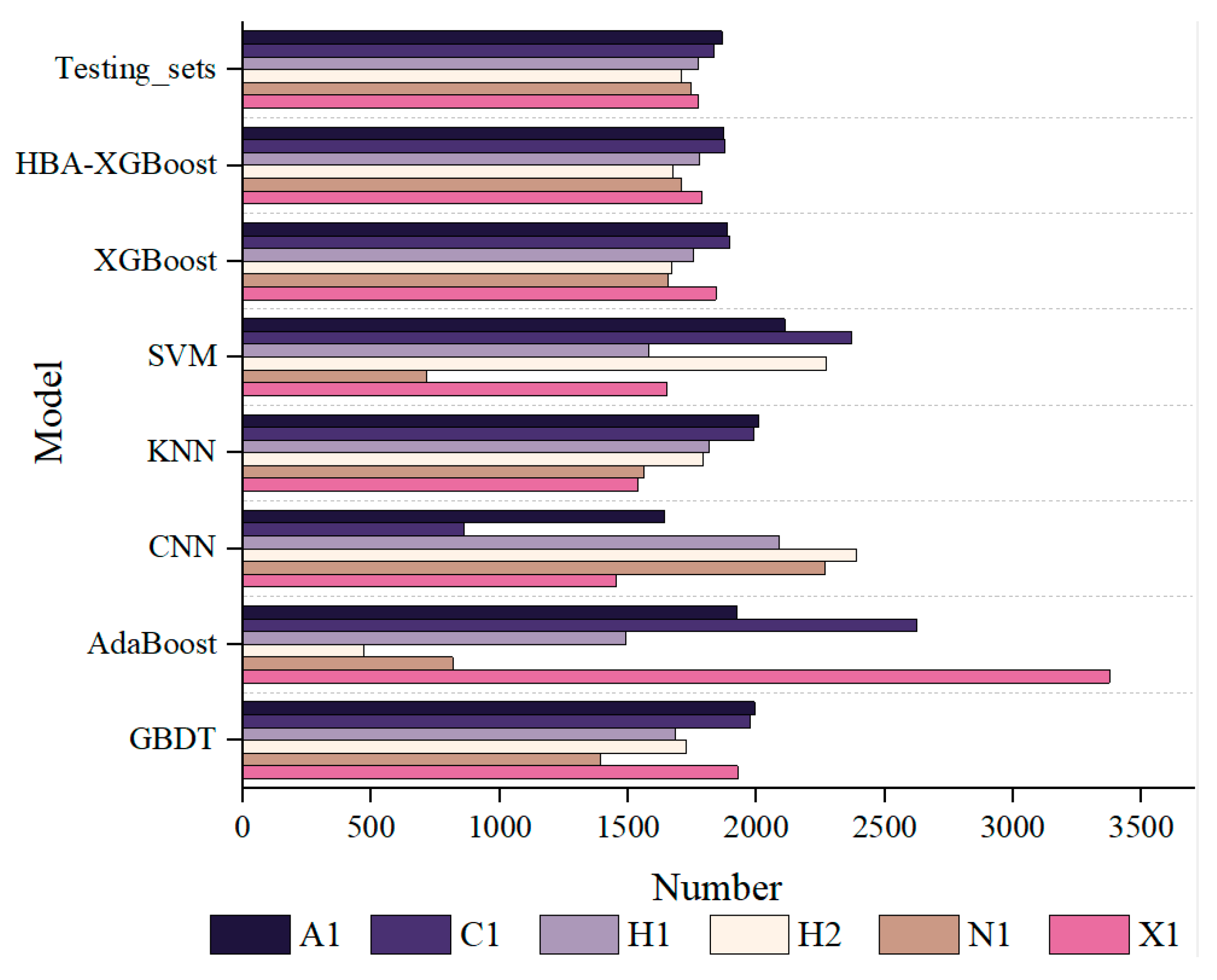
5.2. Model Comparison

In order to highlight the performance of the proposed HBA-XGBoost model, the six models XGBoost, GBDT, AdaBoost, KNN, SVM and CNN were selected, and the same data set was trained via five-fold cross-validation. The performance of the HBA-XGBoost model was compared with that of the other six models. Among them, HBA-XGBoost, XGBoost, GBDT and AdaBoost models are all integrated models using a Boosting algorithm. KNN and SVM are machine learning models identified as having a better lithology recognition effect in previous studies [42,43,44,45]. CNN is a deep learning algorithm that has recently seen a great deal of use and has remarkable effects in computer vision, natural language processing and other fields.
Figure 7 shows the comparison between the prediction results of the different models and the test set. Among them, the HBA-XGBoost model proposed in this paper had the best effect, followed by the XGBoost model. Although AdaBoost and GBDT are also integrated based on a Boosting algorithm, the prediction results were poor. The lithology of H2 and X1 predicted by the AdaBoost model deviated seriously from the real value, and KNN had a higher prediction accuracy than the SVM model. Although convolutional neural networks have demonstrated powerful capabilities in many fields, they are not necessarily superior to classical machine learning algorithms for small and medium-sized table-type data. This is because in these cases the number of features in the data set is small and the convolution kernel set in the convolution operation is small, so it is difficult to fully perceive the features of the data neighborhood, which also leads to an increase in the time of the convolution operation. Figure 8 is a confusion matrix based on real lithology and predicted lithology. Taking the HBA-XGBoost model as an example, the prediction accuracy of the C1 lithology was the highest—where 1% of the proportion was predicted as other lithologies. The worst prediction result was the H2 lithology, where 8% of the proportion was predicted as other lithologies. The main reason for these errors is that the corresponding characteristics of logging between different lithologies are intertwined, which makes lithology identification more difficult. Table 5 lists the specific performance indicators of the different models. The accuracy of HBA-XGBoost was the highest, reaching 96%. Compared with the untuned XGBoost model, the accuracy was increased by 3%. The model effects of KNN, GBDT and CNN were second, and the effects of the support vector machine and AdaBoost models were poor.

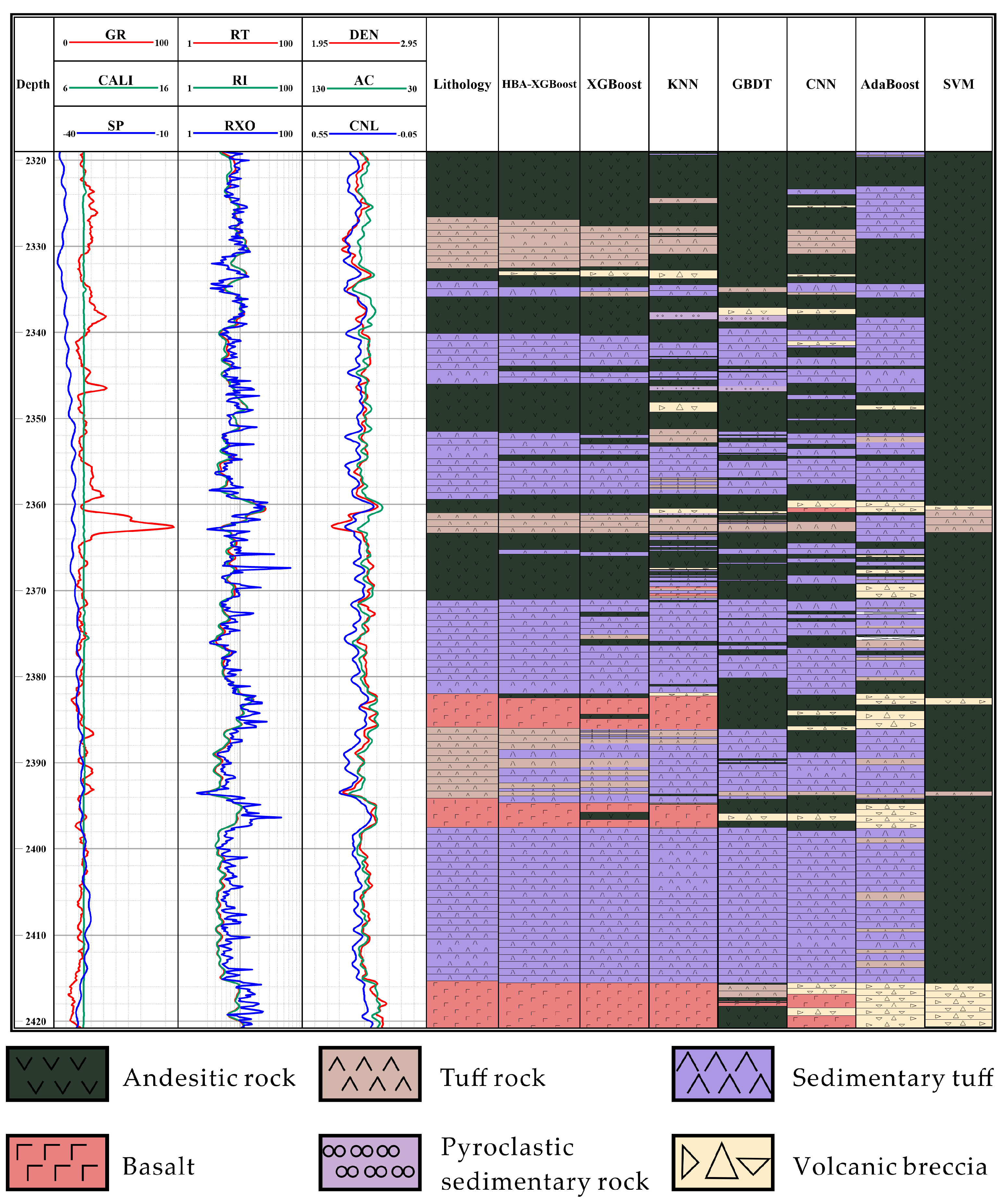
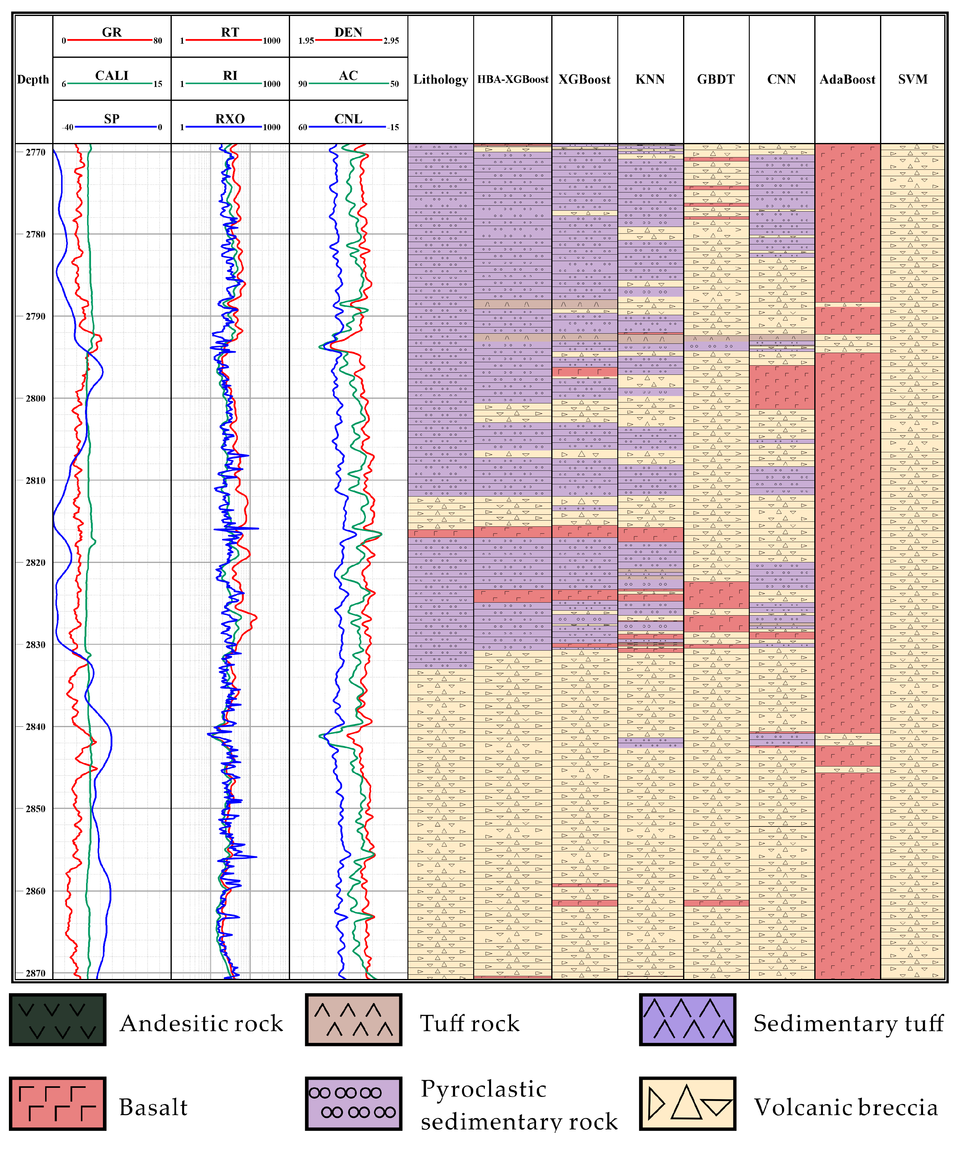
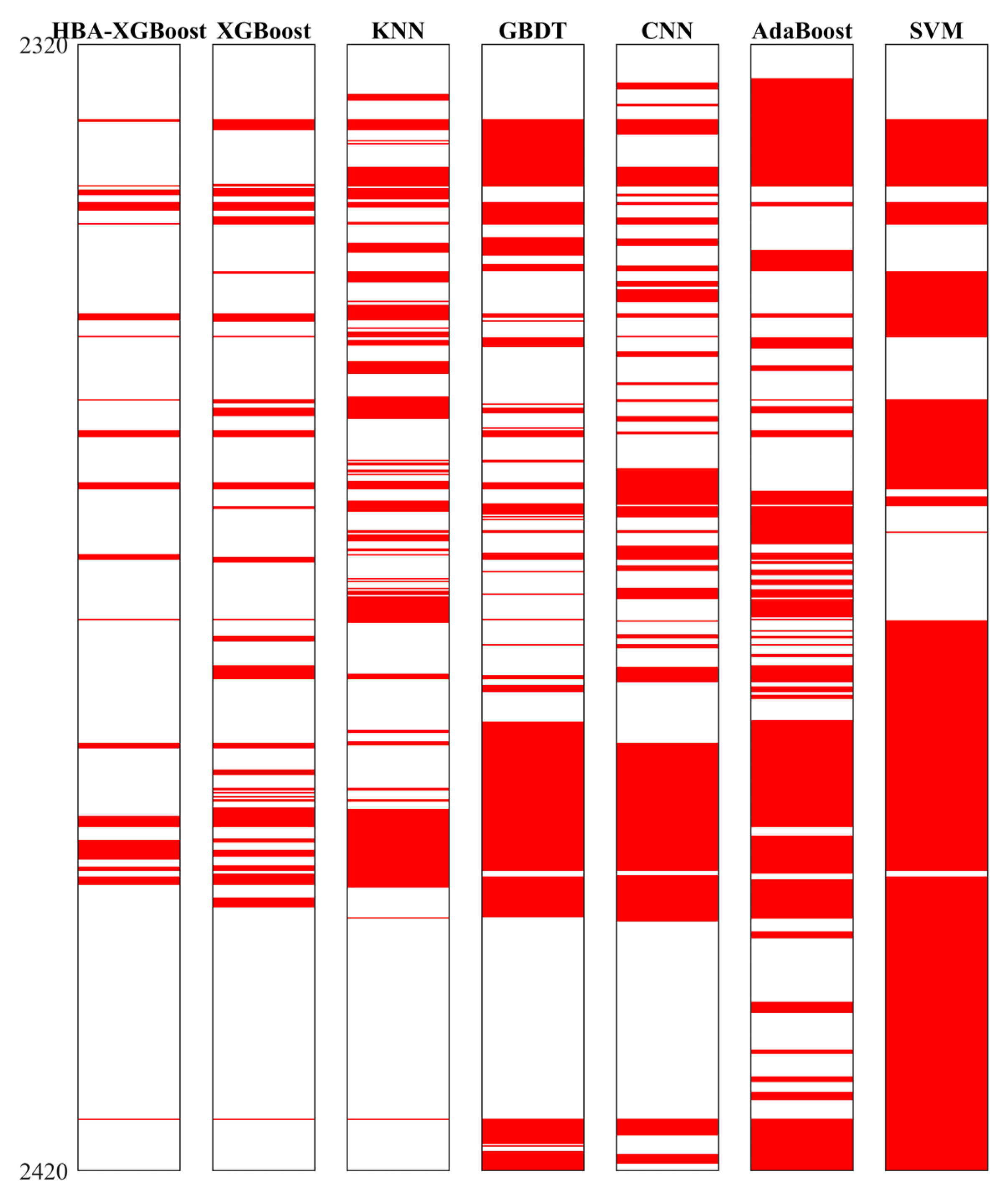
5.3. Practical Application Effect

By quantitatively analyzing the performance indicators of the HBA-XGBoost model and the other six models, it can be said that the HBA-XGBoost volcanic rock lithology identification model has stability and accuracy. On this basis, in order to evaluate the applicability of the HBA-XGBoost model, the Carboniferous volcanic rock strata of well A and well B, which were not involved in the training in the Hongche fault zone, were selected for verification, and the recognition effect of the HBA-XGBoost model was compared with the recognition effect of the six other models. For wells with missing curves, intelligent algorithms can be used to complete the curves [46,47]. The results shown below show that it is feasible to use the HBA-XGBoost model to identify volcanic lithologies. In Figure 9 and Figure 10, the first channel is the depth channel, the second to fourth are the conventional log curve channels, the fifth is the real lithology channel and the sixth to twelfth are the identification results of the seven models.
The main dominant lithologies of well A are andesite, tuff, sedimentary tuff and basalt. In addition to the AdaBoost model and the radial-basis SVM model, other machine learning models roughly predicted the trend of lithology change from top to bottom. The GBDT model predicted andesite when the ground truth was basalt. KNN and CNN’s prediction results showed multiple thin-layer when predicting thick formations. The prediction results of the HBA-XGBoost model and the XGBoost model were higher, but these models could not clearly distinguish between sedimentary tuff and tuff. This is because sedimentary tuff contains 50–90% tuff and the rest is normal sedimentary material, which is similar in log response characteristics, so there was a certain prediction error. The prediction results of the HBA-XGBoost model were closer to the real lithology. The main dominant lithologies of well B are pyroclastic sedimentary rock and volcanic breccia. The prediction results of the latter three models had great errors deviating from the real lithology. GBDT could not distinguish between sedimentary tuff and volcanic breccia. AdaBoost basically predicted the lithology in the depth section as basalt, and SVM basically predicted the lithology in the depth section as volcanic breccia. The prediction accuracy of the HBA-XGBoost model, the XGBoost model, the KNN model and the CNN model decreased in turn and the prediction accuracy of thin-layer lithology increased in the same order.
Figure 11 and Figure 12 reflect the prediction error of the models; The red areas are the depths where the models made incorrect predictions. It can be clearly seen that the prediction effects of the models decreased in the following order: HBA-XGBoost > XGBoost > KNN > GBDT, CNN, AdaBoost > SVM. Through the comparison of actual well prediction, it can be said that the HBA-XGBoost model can be applied to volcanic rock lithology prediction.

6. Discussion and Prospects

In this study, eight conventional curves were used as the input of the HBA-XGBoost model to accurately identify the lithologies of six volcanic rocks in the Carboniferous reservoir of the Hongche fault zone, and the identification effect was better than that obtained using the lithology identification map classification method [33] and other classical machine learning algorithms. Volcanic rocks have significant regional and heterogeneous properties and complex structural components, leading to fuzzy log characteristics. The model proposed in this paper can predict the lithology of volcanic rocks well, and can also be used to distinguish the lithologies of clastic rocks whose diagenesis is relatively simple. In addition to lithology identification, the model can also be applied to oil–water layer identification, interlayer identification, sedimentary facies classification and other fields.
The application effect of the AI model will be affected by the data type, data size, geological region and other factors. Currently, geological data are subregional, and better results may not be obtained if the established models are directly applied to other regions. Therefore, in the follow-up work, the strategy of transfer learning can be adopted to simplify the training process by using small sample data sets in other areas, and by slightly adjusting the model parameters to adapt the model to other research areas. The data used in this paper are all numerical, and other types of data, such as image type and text type, will be generated in the logging process, which means that the data pre-processing process will be more complicated when classifying other types of data, and the analysis and prediction of multi-type and multi-feature data volume types will be the next research trend.

7. Conclusions

The lithology of Carboniferous reservoir volcanic rocks in the Hongche fault zone is complex and changeable, and the accuracy of traditional lithology identification charts is low. In order to solve this problem, this paper proposes a lithology identification model based on HBA-XGBoost. The main conclusions are as follows:
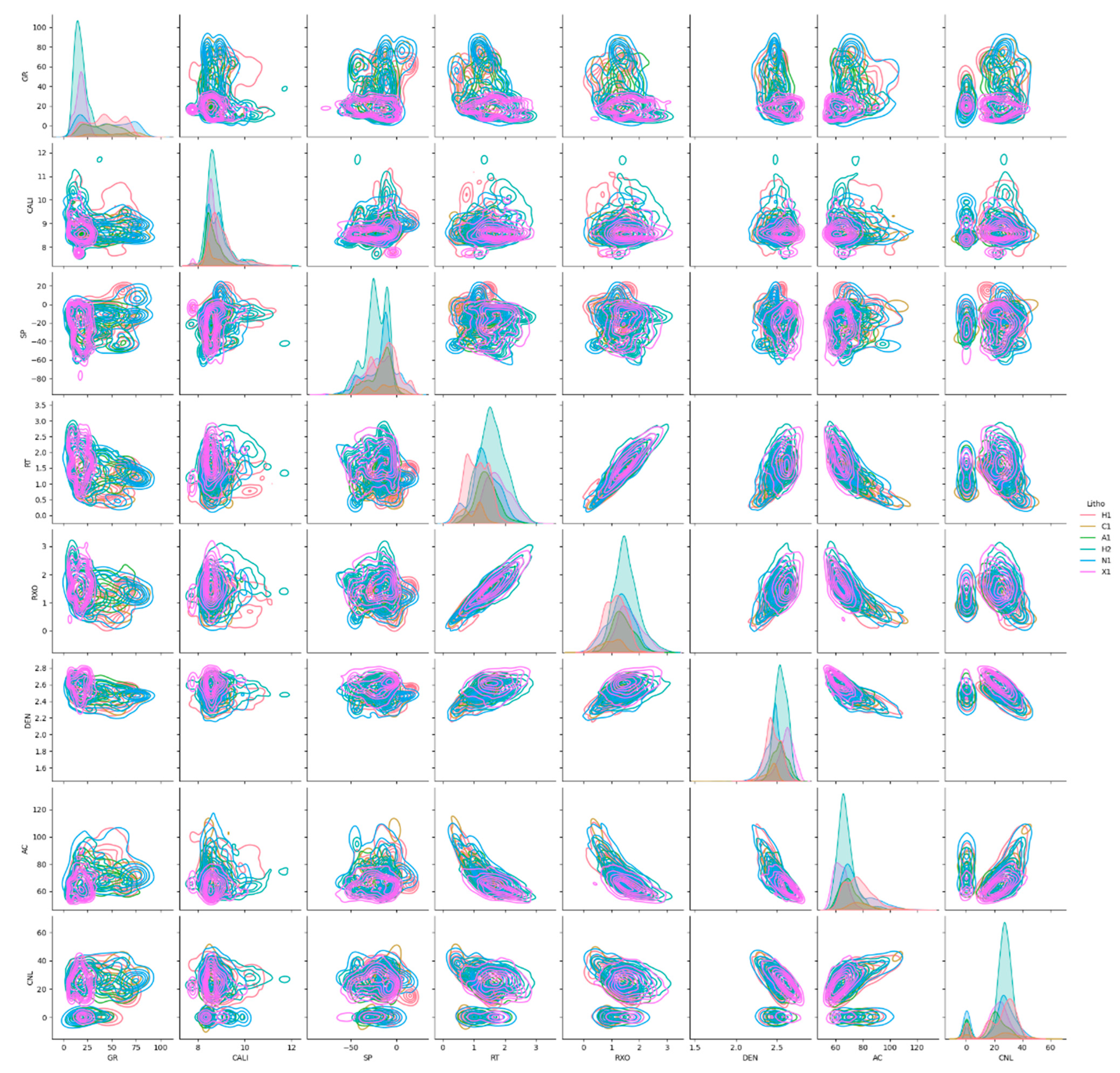
  • Based on the log data of the Hongche fault zone, a volcanic rock lithology data set was established. The data set includes eight curve features: GR, CALI, SP, RT, RXO, DEN, AC and CNL. There are six dominant lithologies: pyroclastic sedimentary rock, volcanic breccia, sedimentary tuff, tuff, andesite and basalt.
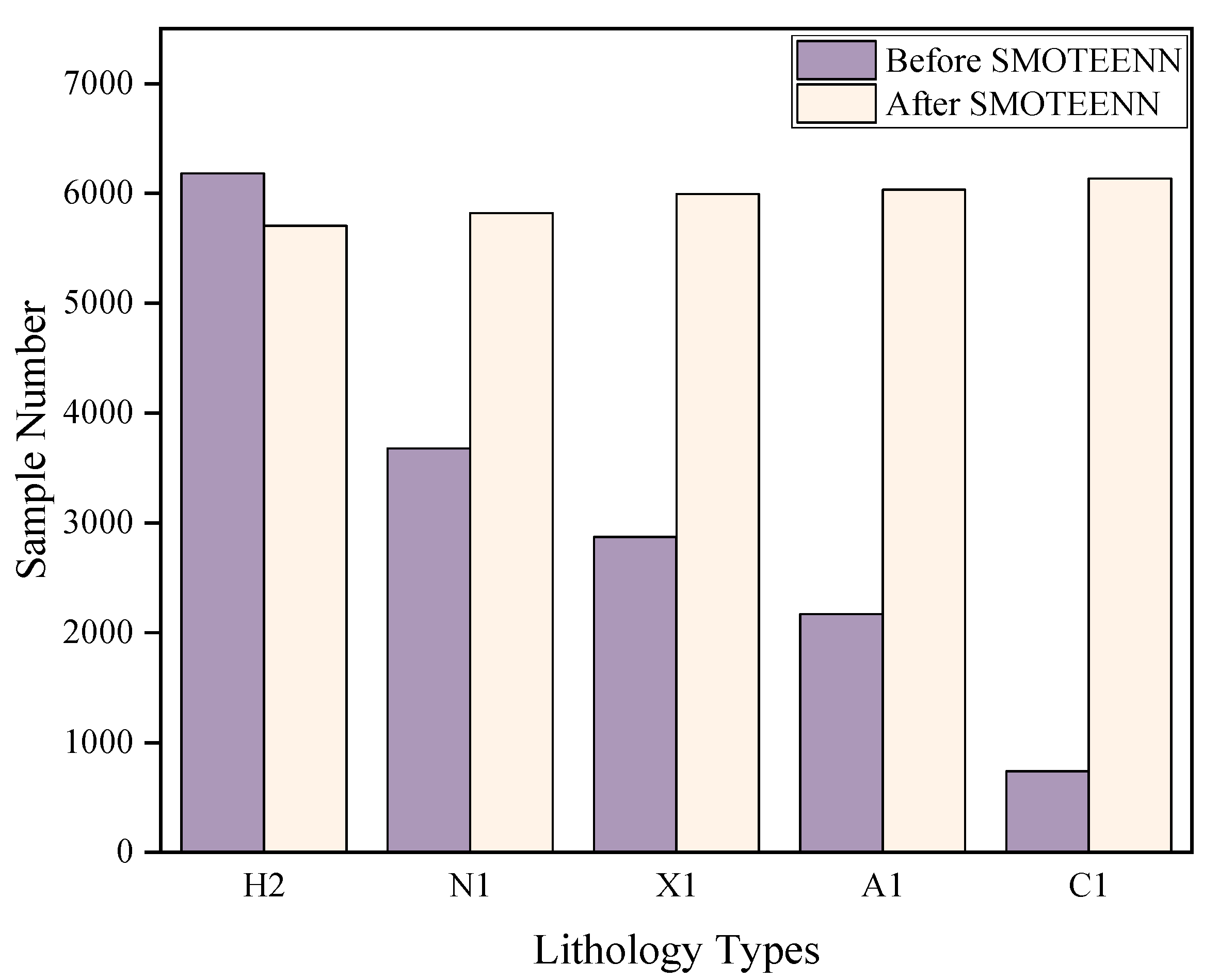
  • SMOTEENN can effectively solve the problem of the unbalanced data scale of different dominant lithologies in a data set, increasing the sample size when there is a small number of samples, reducing the sample size when there is a large number of samples, and balancing the amount of data for various lithology labels.
  • The HBA model can optimize the hyperparameter space of XGBoost, obtain the optimal hyperparameter combination of XGBoost, optimize the model structure of XGBoost and improve the indicators of the XGBoost model in volcanic rock lithology prediction. The overall prediction accuracy was improved by about 3%. The recognition accuracy of HBA-XGBoost for various lithologies in the study area was above 92%, whick is higher than the prediction accuracy of XGBoost, KNN, GBDT, AdaBoost, CNN and SVM.
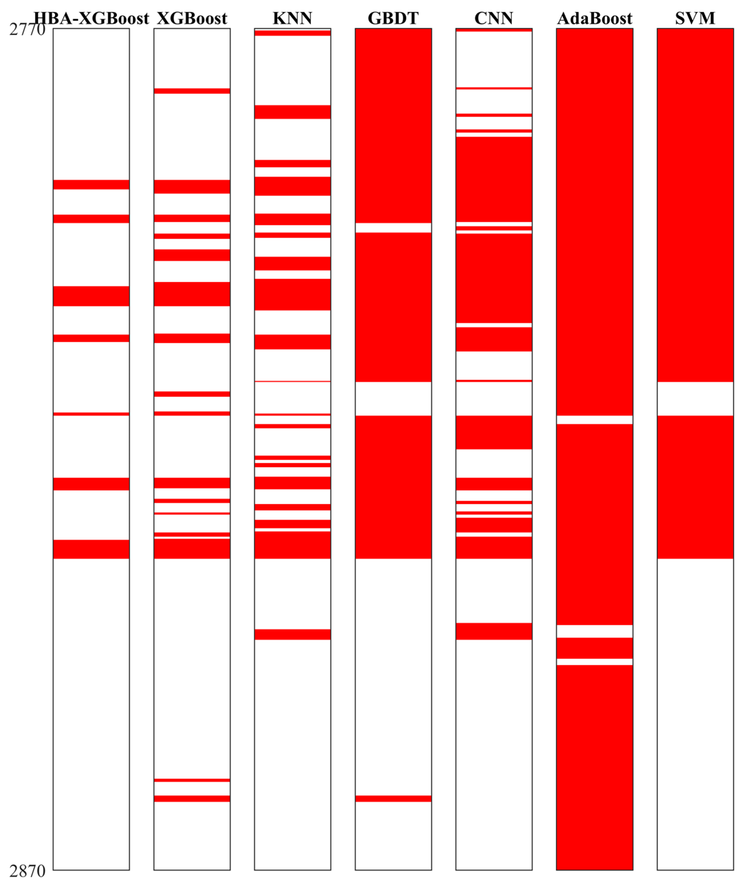
  • The proposed model was applied to the lithology identification of data from two actual wells in the study area. The HBA-XGBoost model accurately and continuously predicted different lithologies, and also accurately predicted at the boundaries of lithology changes. Compared with other models, the prediction accuracy was higher, and provides a certain reference for the lithology identification of volcanic rocks.

Author Contributions

Software, X.S.; Validation, Z.F. and X.Z.; Formal analysis, L.Z.; Writing—original draft, J.C. and C.F.; Writing—review & editing, J.C. and C.F.; Supervision, X.D.; Project administration, C.F. All authors have read and agreed to the published version of the manuscript.

Funding

This research was supported by the Natural Science Foundation of Xinjiang Uygur Autonomous Region (No. 2021D01E22), the Innovative Outstanding Young Talents of Karamay, the Innovative Environmental Construction Plan (Innovative Talents) of Science and Technology Planning project of Karamay (No. 20212022hjcxrc0033) and the National Natural Science Foundation of China (No. 42004089, 42364007).

Data Availability Statement

The data used to support the results of this study are included within the manuscript.

Acknowledgments

All the authors would like to thank the reviewers and editors for their thoughtful comments that greatly improved the manuscript.

Conflicts of Interest

Xili Deng was employed by PetroChina. Xin Shan was employed by North China University of Technology. The remaining authors declare that the research was conducted in the absence of any commercial or financial relationships that could be construed as a potential conflict of interest.

References

  1. Sun, J.; Li, Q.; Chen, M.; Ren, L.; Huang, G.; Li, C.; Zhang, Z. Optimization of models for a rapid identification of lithology while drilling-A win-win strategy based on machine learning. J. Pet. Sci. Eng. 2019, 176, 321–341. [Google Scholar] [CrossRef]
  2. Dev, V.A.; Eden, M.R. Formation lithology classification using scalable gradient boosted decision trees. Comput. Chem. Eng. 2019, 128, 392–404. [Google Scholar] [CrossRef]
  3. Chen, H.Q.; Shi, W.W.; Du, Y.J.; Deng, X.J. Advances in volcanic facies research of volcanic reservoir. Chin. J. Geol. (Sci. Geol. Sin.) 2022, 4, 1307–1323. [Google Scholar]
  4. He, Z.J.; Zeng, Q.C.; Chen, S.; Dai, C.M.; Wang, X.J.; Yang, Y.D. Volcanic reservoir prediction method and application in the Well Yongtan 1, southwest Sichuan. Sci. Technol. Eng. 2021, 21, 10661–10669. [Google Scholar]
  5. Xie, Y.X.; Zhu, C.Y.; Zhou, W.; Li, Z.D.; Liu, X.; Tu, M. Evaluation of machine learning methods for formation lithology identification: A comparison of tuning processes and model performances. J. Pet. Sci. Eng. 2018, 160, 182–193. [Google Scholar] [CrossRef]
  6. Zhang, Y.; Pan, B.Z. Application of SOM Neural Network Method to Volcanic Lithology Recognition Based on Principal Components Analysis. Well Logging Technol. 2009, 33, 550–554. [Google Scholar]
  7. Zhu, Y.X.; Shi, G.R. Identification of lithologic characteristics of volcanic rocks by support vector machine. Acta Pet. Sin. 2013, 34, 312–322. [Google Scholar]
  8. Zhang, Y.; Pan, B.Z. The Application of SVM and FMI to the Lithologic Identification of Volcanic Rocks. Geophys. Geochem. Explor. 2011, 35, 634–638+642. [Google Scholar]
  9. Wang, P.; Wang, Z.Q.; Ji, Y.L.; Duan, W.H.; Pan, L. Identification of Volcanic Rock Based on Kernel Fisher Dis-criminant Analysis. Well Logging Technol. 2015, 39, 390–394. [Google Scholar]
  10. Wang, H.F.; Jiang, Y.L.; Lu, Z.K.; Wang, Z.W. Lithologic identification and application for igneous rocks in eastern depression of Liaohe oil field. World Geol. 2016, 35, 510–516+525. [Google Scholar]
  11. Ye, T.; Wei, A.J.; Deng, H.; Zeng, J.C.; Gao, K.S.; Sun, Z. Study on volcanic lithology identification methods based on the data of conventional well logging data: A case from Mesozoic volcanic rocks in Bohai bay area. Prog. Geophys. 2017, 32, 1842–1848. [Google Scholar]
  12. Xiang, M.; Qin, P.B.; Zhang, F.W. Research and application of logging lithology identification for igneous reservoirs based on deep learning. J. Appl. Geophys. 2020, 173, 103929. [Google Scholar]
  13. Mou, D.; Zhang, L.C.; Xu, C.L. Comparison of Three Classical Machine Learning Algorithms for Lithology Identification of Volcanic Rocks Using Well Logging Data. J. Jilin Univ. (Earth Sci. Ed.) 2021, 51, 951–956. [Google Scholar]
  14. Yang, X.; Wang, Z.Z.; Zhou, Z.Y.; Wei, Z.C.; Qu, K.; Wang, X.Y.; Wang, R.Y. Lithology classification of acidic volcanic rocks based on parameter-optimized AdaBoost algorithm. Acta Pet. Sin. 2019, 40, 457–467. [Google Scholar]
  15. Han, R.Y.; Wang, Z.W.; Wang, W.H.; Xu, F.H.; Qi, X.H.; Cui, Y.T. Lithology identification of igneous rocks based on XGboost and conventional logging curves, a case study of the eastern depression of Liaohe Basin. J. Appl. Geophys. 2021, 195, 104480. [Google Scholar]
  16. Han, R.Y.; Wang, Z.W.; Wang, W.H.; Xu, F.H.; Qi, X.H.; Cui, Y.T.; Zhang, Z.T. Igneous rocks lithology identification with deep forest: Case study from eastern sag, Liaohe basin. J. Appl. Geophys. 2023, 208, 104892. [Google Scholar] [CrossRef]
  17. Sun, Y.S.; Huang, Y.; Liang, T.; Ji, H.C.; Xiang, P.F.; Xu, X.R. Identification of complex carbonate lithology by logging based on XGBoost algorithm. Lithol. Reserv. 2020, 32, 98–106. [Google Scholar]
  18. Yu, Z.C.; Wang, Z.Z.; Zeng, F.C.; Song, P.; Baffour, B.A.; Wang, P.; Wang, W.F.; Li, L. Volcanic lithology identification based on parameter-optimized GBDT algorithm: A case study in the Jilin Oilfield, Songliao Basin, NE China. J. Appl. Geophys. 2021, 194, 104443. [Google Scholar] [CrossRef]
  19. Zhang, C.; Pan, M.; Hu, S.Q.; Hu, Y.F.; Yan, Y.Q. A machine learning lithologic identification method combined with vertical reservoir information. Bull. Geol. Sci. Technol. 2023, 42, 289–299. [Google Scholar]
  20. Liu, M.J.; Li, H.T.; Jiang, Z.B. Application of genetic-BP neural network model in lithology identification by logging data in Binchang mining area. Coal Geol. Explor. 2011, 39, 8–12. [Google Scholar]
  21. Ren, Q.; Zhang, H.B.; Zhang, D.L.; Zhao, X. Lithology identification using principal component analysis and particle swarm optimization fuzzy decision tree. J. Pet. Sci. Eng. 2023, 220, 111233. [Google Scholar] [CrossRef]
  22. Zhang, T.; Li, Y.P.; Liu, X.Y.; Li, M.Y.; Wang, J.J. Lithology interpretation of deep metamorphic rocks with well logging based on APSO-LSSVM algorithm. Prog. Geophys. 2022, 38, 382–392. [Google Scholar]
  23. Zhang, J.L.; He, Y.B.; Zhang, Y.; Li, W.F.; Zhang, J.J. Well-Logging-Based Lithology Classification Using Machine Learning Methods for High-Quality Reservoir Identification: A Case Study of Baikouquan Formation in Mahu Area of Junggar Basin, NW China. Energies 2022, 15, 3675. [Google Scholar] [CrossRef]
  24. Sun, Z.X.; Jiang, B.S.; Li, X.L.; Li, J.K.; Xiao, K. A data-driven approach for lithology identification based on parameter-optimized ensemble learning. Energies 2020, 13, 3903. [Google Scholar] [CrossRef]
  25. Andic, C.; Ozumcan, S.; Ozturk, A.; Turkay, B. Honey Badger Algorithm Based Tuning of PID Conroller for Load Frequency Control in Two-Area Power System Including Electric Vehicle Battery. In Proceedings of the 2022 4th Global Power, Energy and Communication Conference (GPECOM), Cappadocia, Turkey, 14–17 June 2022; IEEE: Piscataway, NJ, USA, 2022; pp. 307–310. [Google Scholar]
  26. Akdağ, O. A Developed Honey Badger Optimization Algorithm for Tackling Optimal Power Flow Problem. Electr. Power Compon. Syst. 2022, 50, 331–348. [Google Scholar] [CrossRef]
  27. Jaiswal, G.K.; Nangia, U.; Jain, N.K. Optimal Reactive Power Dispatch Using Honey Badger algorithm (HBA). In Proceedings of the 2022 IEEE 10th Power India International Conference (PIICON), New Delhi, India, 25–27 November 2022; IEEE: Piscataway, NJ, USA, 2022; pp. 1–6. [Google Scholar]
  28. Su, P.D.; Qin, Q.R.; Yuan, Y.F.; Jiang, F.D. Characteristics of Volcanic Reservoir Fractures in Upper Wall of HongChe Fault Belt. Xinjiang Pet. Geol. 2011, 32, 457–460. [Google Scholar]
  29. Liu, Y.; Wu, K.Y.; Wang, X.; Liu, B.; Guo, J.X.; Du, Y.N. Architecture of buried reverse fault zone in the sedimentary basin: A case study from the Hong-Che Fault Zone of the Junggar Basin. J. Struct. Geol. 2017, 105, 1–17. [Google Scholar] [CrossRef]
  30. Jiang, Q.J.; Li, Y.; Liu, X.J.; Wang, J.; Ma, W.Y.; He, Q.B. Controlling factors of multi-source and multi-stage complex hydrocarbon accumulation and favorable exploration area in the Hongche fault zone, Junggar Basin. Nat. Gas Geosci. 2023, 34, 807–820. [Google Scholar]
  31. Gan, X.Q.; Jiang, Y.Y.; Qin, Q.R.; Song, W.Y. Characteristics of the Carboniferous volcanic reservoir in the Hongche fault zone. Spec. Oil Gas Reserv. 2011, 18, 45–17+137. [Google Scholar]
  32. Yao, W.J.; Dang, Y.F.; Zhang, S.C.; Zhi, D.M.; Xing, C.Z.; Shi, J.A. Formation of Carboniferous Reservoir in Hongche Fault Belt, Northwestern Margin of Junggar Basin. Nat. Gas Geosci. 2010, 21, 917–923. [Google Scholar]
  33. Feng, Z.Y.; Yin, W.; Zhong, Y.T.; Yu, J.; Zhao, L.; Feng, C. Lithologic identification of igneous rocks based on conventional log: A case study of Carboniferous igneous reservoir in Hongche Fault Zone in Northwestern Junggar Basin. J. Northeast Pet. Univ. 2021, 45, 95–108. [Google Scholar]
  34. Dong, X.M.; Li, J.; Pan, T.; Xu, Q.; Chen, L.; Ren, J.M.; Jin, K. Hydrocarbon accumulation conditions and exploration potential of Hongche fault zone in Junggar Basin. Acta Pet. Sin. 2023, 44, 748–764. [Google Scholar]
  35. Zhong, W.J.; Huang, X.H.; Zhang, Y.H.; Jia, C.M.; Wu, K.Y. Structural characteristics and reservoir forming control of Hongche fault zone in Junggar Basin. Complex Hydrocarb. Reserv. 2018, 11, 1–5. [Google Scholar]
  36. Fan, C.H.; Qin, Q.R.; Yuan, Y.F.; Wang, X.D.; Zhu, Y.P. Structure characteristics and fracture development pattern of the Carboniferous in Hongche fracture belt. Spec. Oil Gas Reserv. 2010, 17, 47–49. [Google Scholar]
  37. Hashim, F.A.; Houssein, E.H.; Hussain, K.; Mabrouk, M.S.; AI-Atabany, W. Honey Badger Algorithm: New metaheuristic algorithm for solving optimization problems. Math. Comput. Simul. 2022, 192, 84–110. [Google Scholar] [CrossRef]
  38. Chen, T.Q.; Carlos, G. XGBoost: A Scalable Tree Boosting System. In Proceedings of the 22nd ACM SIGKDD International Conference on Knowledge Discovery and Data Mining, San Francisco, CA, USA, 13–17 August 2016; pp. 785–794. [Google Scholar]
  39. Friedman, J.H. Greedy Function Approximation: A Gradient Boosting Machine. Ann. Stat. 2001, 29, 1189–1232. [Google Scholar] [CrossRef]
  40. Fu, G.M.; Yan, J.Y.; Zhang, K.; Hu, H.; Luo, F. Current status and progress of lithology identification technology. Prog. Geophys. 2017, 32, 26–40. [Google Scholar]
  41. Muntasir Nishat, M.; Faisal, F.; Jahan Ratul, I.; Al-Monsur, A.; Ar-Rafi, A.M.; Nasrullah, S.M.; Khan, M.R.H. A comprehensive investigation of the performances of different machine learning classifiers with SMOTE-ENN over-sampling technique and hyperparameter optimization for imbalanced heart failure dataset. Sci. Program. 2022, 2022, 3649406. [Google Scholar]
  42. Zou, Y.; Chen, Y.; Deng, H. Gradient boosting decision tree for lithology identification with well logs: A case study of zhaoxian gold deposit, shandong peninsula, China. Nat. Resour. Res. 2021, 30, 3197–3217. [Google Scholar] [CrossRef]
  43. Lai, Q.; Wei, B.Y.; Wu, Y.Y.; Pan, B.Z.; Xie, B.; Guo, Y.H. Classification of Igneous Rock Lithology with K-nearest Neighbor Algorithm Based on Random Forest (RF-KNN). Spec. Oil Gas Reserv. 2021, 28, 62–69. [Google Scholar]
  44. Asante-Okyere, S.; Shen, C.; Osei, H. Enhanced machine learning tree classifiers for lithology identification using Bayesian optimization. Appl. Comput. Geosci. 2022, 16, 100100. [Google Scholar] [CrossRef]
  45. Liang, H.B.; Chen, H.F.; Guo, J.H.; Bai, J.; Jiang, Y.J. Research on lithology identification method based on mechanical specific energy principle and machine learning theory. Expert Syst. Appl. 2022, 189, 116142. [Google Scholar] [CrossRef]
  46. Han, J.; Lu, C.H.; Cao, Z.M.; Mu, H.W. Integration of deep neural networks and ensemble learning machines for missing well logs estimation. Flow Meas. Instrum. 2020, 73, 101748. [Google Scholar]
  47. Tariq, Z.; Elkatatny, S.; Mahmoud, M.; Abdulraheem, A. A new artificial intelligence based empirical correlation to predict sonic travel time. In Proceedings of the 2016 International Petroleum Technology Conference, Bangkok, Thailand, 14–16 November 2016. [Google Scholar]
Figure 1. Structural location map of the Hongche fault zone.
Processes 12 00285 g001
Figure 2. Flow chart of establishing the HBA-XGBoost model.
Processes 12 00285 g002
Figure 3. Two-dimensional nuclear density maps of different lithologies.
Processes 12 00285 g003
Figure 4. Comparison of the number of different lithology samples before and after SMOTEENN sampling.
Processes 12 00285 g004
Figure 5. HBA optimization iterative process.
Processes 12 00285 g005
Figure 6. Confusion matrix of the HBA-XGBoost model.
Processes 12 00285 g006
Figure 7. Comparison of the evaluated models’ prediction results for different lithologies.
Processes 12 00285 g007
Figure 8. Confusion matrices of different models: (a) HBA-XGBoost, (b) XGBoost, (c) GBDT, (d) KNN, (e) CNN, (f) SVM, (g) AdaBoost.
Processes 12 00285 g008
Figure 9. The application of the different models in well A.
Processes 12 00285 g009
Figure 10. The application of the different models in well B.
Processes 12 00285 g010
Figure 11. The prediction error of the different models in well A. (The red areas are the depths where the models made incorrect predictions).
Processes 12 00285 g011
Figure 12. The prediction error of the different models in well B. (The red areas are the depths where the models made incorrect predictions).
Processes 12 00285 g012
Table 1. Confusion matrix diagram.
True LabelPredicted Label
PositiveNegative
PositiveTP (True Positive)FN (False Negative)
NegativeFP (False Positive)TN (True Negative)
Table 2. Log response range of different lithologies (RT and RXO data have been log-transformed).
GRCALISPRTRXODENACCNL
H17.89~92.257.66~11.66−45.81~18.000.21~2.36−0.06~2.652.01~2.7554.61~127.920.13~49.82
(43.24)(8.98)(−13.60)(1.10)(1.11)(2.45)(76.88)(24.54)
N16.02~95.287.66~10.68−67.67~22.200.10~2.75−0.36~2.081.75~2.7856.16~124.060.16~53.44
(43.20)(8.84)(−16.26)(1.34)(1.31)(2.45)(75.36)(22.60)
H23.75~75.677.63~12.02−63.02~17.090.41~2.970.21~3.242.18~2.7752.94~102.120.17~46.10
(19.77)(8.83)(−22.69)(1.59)(1.52)(2.54)(67.64)(26.50)
A17.63~88.128.07~10.14−52.17~10.920.46~2.680.02~3.022.18~2.8153.54~98.290.10~41.17
(39.35)(8.65)(−18.13)(1.41)(1.40)(2.53)(69.64)(17.51)
X15.15~95.787.64~10.91−85.20~1.160.33~3.27−0.20~3.212.10~2.8352.00~107.240.09~46.36
(18.04)(8.65)(−23.84)(1.72)(1.65)(2.60)(63.61)(22.04)
C115.99~89.408.17~9.84−61.93~16.460.22~1.74−0.36~2.461.55~2.5860.76~120.880.23~56.06
(54.73)(8.63)(−13.10)(0.93)(1.00)(2.40)(82.05)(23.57)
The format of the data in the table is: minimum   value   ~   maximum   value ( average   value ) .
Table 3. Default value and significance of different hyperparameters in the XGBoost model.
HyperparameterDefault ValueHyperparameter Meaning Region of SearchGlobal Optimum
n_estimators100Number of weak classifiers[50~200]196
learning_rate0.3Learning rate[0.01~1.0]0.4987
subsample1Proportion of samples taken from a sample[0.5~1.0]0.8154
max_depth6Maximum weak classifier depth [3~10]9
gamma0Decrease of the minimum objective function required for weak classifier branching[0~5]0
min_child_weight1Minimum sample weight required on the leaf node of the weak classifier[0.01~10]0.01
colsample_bytree1Proportion of features extracted by constructing a weak classifier for all features[0.5~1.0]0.97
Table 4. Performance evaluation of the HBA-XGBoost model.
Precision (%)Recall (%)F1-Score (%)Accuracy (%)
A196.9197.3297.1195.70
C197.0299.2998.14
H196.2396.3496.28
H293.8092.0492.91
N194.8592.8493.84
X195.1496.0095.57
Mean value95.6695.6495.64
Table 5. Performance analysis of different models.
ModelPerformance
Index
A1C1H1H2N1X1Mean
Value
Accuracy
HBA-XGBoostPrecision0.970.970.960.940.950.950.960.96
Recall0.970.990.960.920.930.960.96
F1-score0.970.980.960.930.940.960.96
XGBoostPrecision0.940.950.940.890.930.910.930.93
Recall0.950.990.930.870.880.940.93
F1-score0.950.970.940.880.90.930.93
KNNPrecision0.850.890.860.840.870.860.860.86
Recall0.910.960.870.750.780.880.86
F1-score0.880.920.860.790.820.870.86
GBDTPrecision0.780.840.790.690.760.750.770.77
Recall0.830.900.750.700.610.810.77
F1-score0.800.870.770.690.680.780.77
CNNPrecision0.730.610.770.770.730.770.730.75
Recall0.710.400.810.830.720.690.69
F1-score0.720.480.790.800.730.730.71
SVMPrecision0.580.630.590.490.630.620.590.58
Recall0.650.820.520.650.260.570.58
F1-score0.610.710.550.560.360.600.57
AdaBoostPrecision0.520.550.360.350.460.420.440.46
Recall0.530.780.300.100.210.800.46
F1-score0.530.640.330.150.290.550.42
Disclaimer/Publisher’s Note: The statements, opinions and data contained in all publications are solely those of the individual author(s) and contributor(s) and not of MDPI and/or the editor(s). MDPI and/or the editor(s) disclaim responsibility for any injury to people or property resulting from any ideas, methods, instructions or products referred to in the content.

