New Method for Logging Evaluation of Total Organic Carbon Content in Shale Reservoirs Based on Time-Domain Convolutional Neural Network

Abstract

Total organic carbon (TOC) content is a key indicator for determining the hydrocarbon content of shale. The current model for calculating the TOC content of shale is relatively simplistic, the modeling process is cumbersome, and the parameters involved are influenced by subjective factors, which have certain shortcomings. To address this problem, a time-domain convolutional neural network (TCN) model for predicting total organic carbon content based on logging sequence information was established by starting from logging sequence information, conducting logging parameter sensitivity analysis experiments, prioritizing logging-sensitive parameters as model feature vectors, and constructing a TCN network. Meanwhile, to overcome the problem of an insufficient sample size, a five-fold cross-validation method was used to train the TCN model and obtain the weight matrix with the minimum error, and then a shale reservoir TOC content prediction model based on the TCN model was established. The model was applied to evaluate the TOC logging of the Lianggaoshan Formation in the Sichuan Basin, China, and the predicted results were compared with the traditional ΔlogR model. The results indicate that the TCN model predicts the TOC content more accurately than the traditional model, as demonstrated by laboratory tests. This leads to a better application effect. Additionally, the model fully explores the relationship between the logging curve and the total organic carbon content, resulting in improved accuracy of the shale TOC logging evaluation.

1. Introduction

As domestic and international oilfield exploration and development continue to deepen, unconventional, hidden, and complex oil and gas reservoirs are increasingly being developed. Shale reservoirs, in particular, have become a primary target for major oilfields seeking to increase their reserves and production. Total organic carbon content represents the mass of organic matter per unit mass of rock, which reflects the abundance of organic matter in the hydrocarbon source rock, as well as the potential for hydrocarbon production, and it is an important parameter in the evaluation of the “geologic sweet spot” of shale reservoirs [1]. It has been demonstrated that an increase in the total organic carbon content of a formation is directly proportional to an increase in the gas content of the same formation [2]. At the same time, the hydrocarbon generation and drainage behavior of shale reservoirs can modify the physical properties of the reservoirs and form micropores and microfractures [3]. This modification can improve the storage capacity of shale reservoirs. In conclusion, the evaluation of organic carbon content is particularly critical in shale due to its self-generated and self-storage nature. Accurately predicting total organic carbon content is a key technology that guides oilfield exploitation and subsequent well deployment.

Laboratory geochemical analysis experiments are generally considered to provide the highest level of confidence in TOC content. However, they have some disadvantages, such as being discrete, having low vertical resolution, being expensive, and not allowing for a continuous characterization of the TOC content of a formation [4]. However, logging data have a high vertical resolution, which can be used to establish a quantitative calculation model based on the response characteristics of TOC content on the logging curve. This model can then be used to determine the TOC content of the entire well section. Currently, both domestic and foreign scholars have developed mature techniques for quantitatively evaluating TOC content in logging. These techniques can be broadly categorized into two groups. The first group is based on analyzing the TOC content scale logging curves with cores, by examining the logging response characteristics and establishing corresponding statistical models. For instance, the ΔlogR method [5] combines the overlap of resistivity and porosity curves with the casein maturity index to quantify TOC content. However, it has certain limitations, due to the difficulty of accurately defining the coefficients in the model and its excessive dependence on the maturity index. In response to these limitations, several scholars have made improvements to the ΔlogR method. Huang et al. [6] used the method of coefficients to obtain a variable-coefficient ΔlogR model for the problem of variable model parameters and poor generalization. Zhou et al. [7] combined the traditional natural gamma method with the ΔlogR method by constructing parameters reflecting the mineral content. This effectively solved the shortcomings of the traditional method. Jacobi et al. [8] combined nuclear magnetic resonance (NMR) logging technology with conventional density logging technology and put forward the corresponding petrophysical volume model, which utilized the difference between density logging and NMR logging to compute porosity, to obtain the casein volume and then calculate the organic carbon content; but for shale formations with a high clay content, it is difficult to accurately determine the skeleton by density logging, and NMR logging, in the mode of long echo spacing measurement, cannot effectively characterize the total porosity of the formation. Evaluating the TOC content of shale using simpler statistical models can be challenging due to its geologic genesis, relatively thin reservoir thickness, and strong non-homogeneous characteristics. The second category refers to machine learning models based on logging data mining. In recent years, computing performance has improved dramatically, and a range of machine learning algorithms based on neural network models have been widely applied to the field of logging. These applications include the quantitative evaluation of reservoir parameters, the classification of pore structure, and the identification of fluid properties. For the prediction of TOC content, several scholars have similarly applied machine learning algorithms. Lu et al. [9] used neural networks to use logging curves as feature vectors and TOC as labels and then built a BP neural network model. Zhu et al. [10] optimized the BP neural network in terms of optimizing the weights before iteration, optimizing the structure of the network, and integrating the strings in parallel, and finally formed a set of hybrid neural network models to predict TOC. Zhu et al. [11] used the curve overlapping algorithm to give geological significance to the prediction model and utilized an integrated deep semi-supervised step network to predict the organic carbon content of hydrocarbon source rocks. Researchers are increasingly viewing geophysical problems as time series problems due to their in-depth understanding. Geophysical logging parameters with different burial depths, geological ages, and depositional characteristics exhibit time series characteristics. Deep learning algorithms, such as the recurrent neural network (RNN), gated recurrent neural network (GRU), long short-term memory recurrent neural network (LSTM), and bi-directional long short-term memory recurrent neural network (Bi-LSTM), are increasingly being used to address timing issues in the logging field [12,13]. All of the aforementioned networks perform well in addressing timing issues. However, they have a disadvantage in their internal design, which can lead to problems such as gradient explosion, gradient disappearance, or high memory usage. To solve this problem, Lea et al. [14] first proposed a time-domain convolutional neural network (TCN) in 2017, which combines a convolutional neural network with a recurrent neural network to solve the shortcomings of the recurrent neural network, and which can also process data in parallel to optimize computer memory occupation. Based on this, this paper builds a TOC prediction model based on a time-domain convolutional neural network based on logging data and verifies the model performance with real data of oil shale from the Lianggaoshan Formation in the Sichuan Basin.

2. Overview of the Methodology

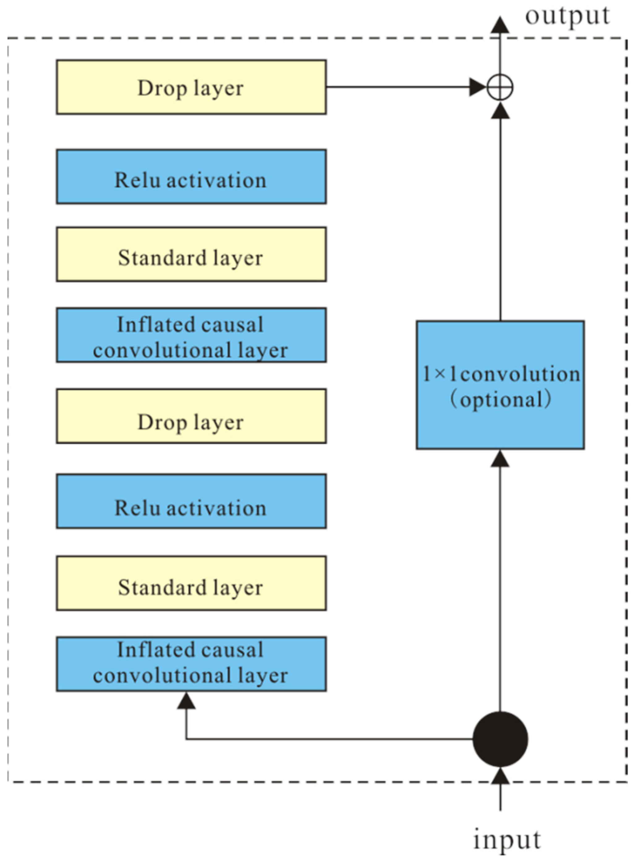
2.1. Time-Domain Convolutional Neural Network

The time-domain convolutional neural network is a generalized architecture for predicting sequences using convolutional networks. It is designed to be simple and memory-enabled, making it suitable for sequence-modeling tasks. The TCN includes several core structures, such as the fully convolutional network (FCN) [15], causal convolution, inflationary convolution, and residual block structure [16]. The fully convolutional network’s hidden layers are zero-padded to match the input layer’s length, resulting in the same input and output dimensions. To enhance the network’s historical memory function, the TCN employs a combination of causal and inflationary convolutions (as shown in Figure 1) to expand its sensory field for historical information.

Figure 2 displays the residual block structure of the TCN. To deepen the TCN model, it is necessary to replace the convolutional layer with a residual connection to enhance stability, as shown in Figure 2. The residual block structure contains two layers of inflated causal convolution, the activation function ReLU (responsible for mapping the inputs of the neuron to the outputs), the discard layer, and the standard layer. Finally, to ensure input and output dimensionality consistency, a one-dimensional full convolution operation maps the input and output. In summary, the TCN model utilizes inflated causal convolutional layers with a specific residual linkage to allow for a flexible sense field (network memory length), better control of the model’s memory size, and avoiding the problem of gradient explosion in recurrent neural networks. The size of the convolution kernel, the expansion factor (parameters responsible for controlling the size of the dilation convolution), and the number of convolution layers determine the receptive field of the TCN network. The expansion convolution operation for the ‘sth’ sequence element in the network can be defined as follows:

$$F(\mathrm{s})=(x*f)(s)={\displaystyle \sum _{i=0}^{k-1}f(i)\cdot }xs-d\cdot i$$

(1)

The input sequence is represented by x, while d represents the expansion factor. The ith element in the convolution kernel is represented by f(i), and * denotes the symbol of the convolution operation. The filter size is represented by k, and ${\mathrm{x}}_{s - d\cdot i}$ represents the element in the input sequence that corresponds to the convolution kernel. The expansion convolution reduces to regular convolution when d = 1. The use of larger convolutions expands the sensory domain of the convolutional layer more effectively. This allows the output of the top layer of the network to represent a wider range of inputs.

Figure 2. Schematic structure of residual block.

Figure 2. Schematic structure of residual block.

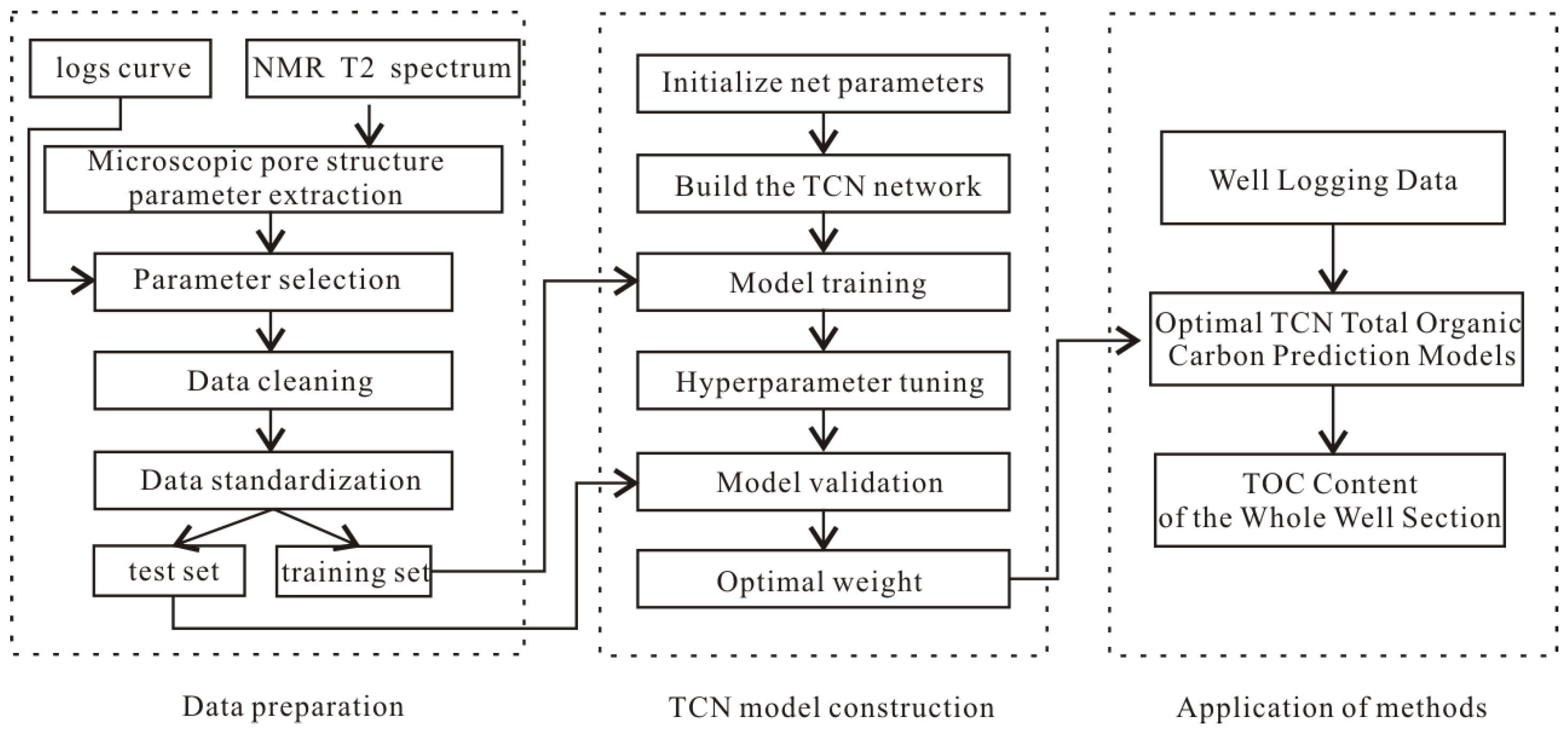
2.2. Evaluation Method of Total Organic Carbon Content Logging Based on TCN Modeling

Figure 3 displays the shale organic carbon content logging evaluation framework based on the TCN model, which comprises three major steps. The first step involves data preparation, utilizing conventional logging data and NMR logging data. The NMR logging T₂ spectrum is used to extract parameters that characterize the reservoir’s microscopic pore structure. Once the extraction is complete, the logging parameters and the real TOC content are correlated and analyzed in the network model. The preferred parameters are those that are sensitive, and the influence of multicollinearity is reduced. After completing parameter optimization, the network input label is the true TOC, and the feature vectors of the network input are the sensitive parameters. The dataset is then cleansed to remove singular values, and the training and test sets are divided proportionally. The next step is to build the TCN model. Once the network is constructed, the initial network parameters are applied, and the training set is fed into the TCN model. The following points must be stated: the real TOC values are obtained through core experiments; the input of the TCN network is based on the set sliding window size to determine the size of each group of inputs, taking into account the continuity of the depth of the ground; this paper will be a group of parameters at multiple depths in the form of a sequence of vectors as inputs, for example, a logging curve with a sampling interval of 0.125 m; the sliding window size is set to 10, then it is 10 vectors as a set of input, so that every interval of 1.25 m corresponds to a TOC value used as a label. The model is then trained using the mean square error (MSE) loss function to evaluate the accuracy of the model’s predictions, as shown in Equation (2). When the model training is completed, the weights, as well as the gradients, in the optimal model are saved as the mapping relationship between logging parameters and TOC content. The third step is the application of the method, where the TOC at a depth point can be obtained by inputting the logging data at that depth point, and eventually the prediction of TOC content for the whole well section can be performed.

$$MSE=\frac{1}{\mathrm{n}}{{\displaystyle \sum (y_i-\stackrel{\wedge }{y_i})}}^2$$

(2)

where n is the total number of samples; $y_i$ is the predicted organic carbon content; ${\stackrel{\wedge }{y}}_i$ is the true organic carbon content.

Figure 3. Logging evaluation framework of shale organic carbon content based on TCN model.

Figure 3. Logging evaluation framework of shale organic carbon content based on TCN model.

3. Experiments and Analyses

3.1. Extraction of NMR T₂ Spectral Parameters

Bai et al. [17] used the graphical method and method of moments, based on normal distribution and geological experience models, to extract microscopic parameters that reflect the pore structure and fluid endowment state in the T2 spectra [18]. The authors extracted these parameters to investigate the connection between TOC content and the microscopic pore structure of the reservoir. These parameters include the geometric mean, spectral peak relaxation time, kurtosis, coefficient of variation, mean value, small porosity component (S1), medium porosity component (S2), and large porosity component (S3). The NMR T2 spectrum contains several microscopic parameters that characterize the pore-sorting features. Figure 4 shows a schematic diagram of the positions of some of these parameters. It is important to note that the diagram does not quantify the microscopic parameters characterizing the pore-sorting features.

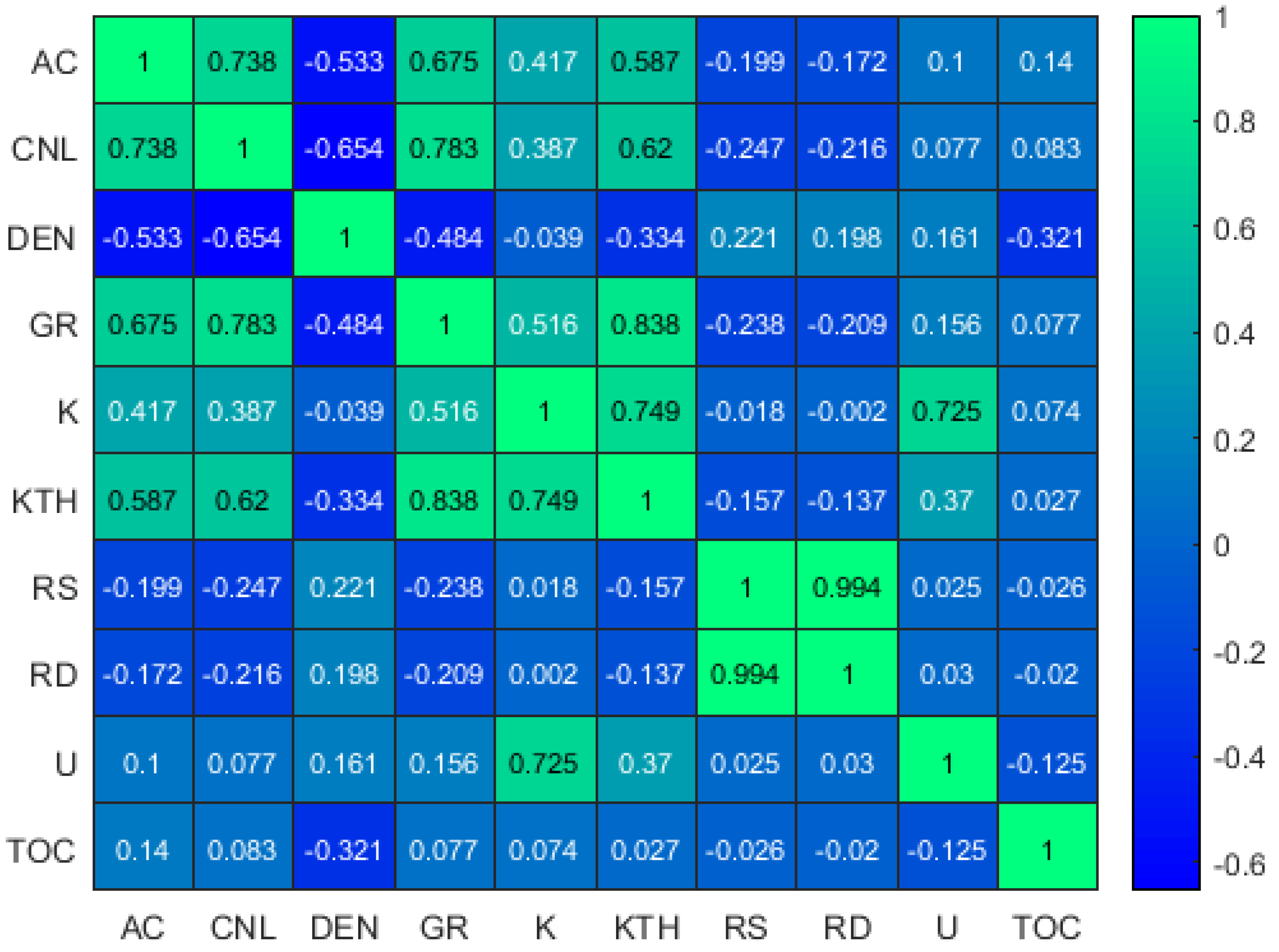
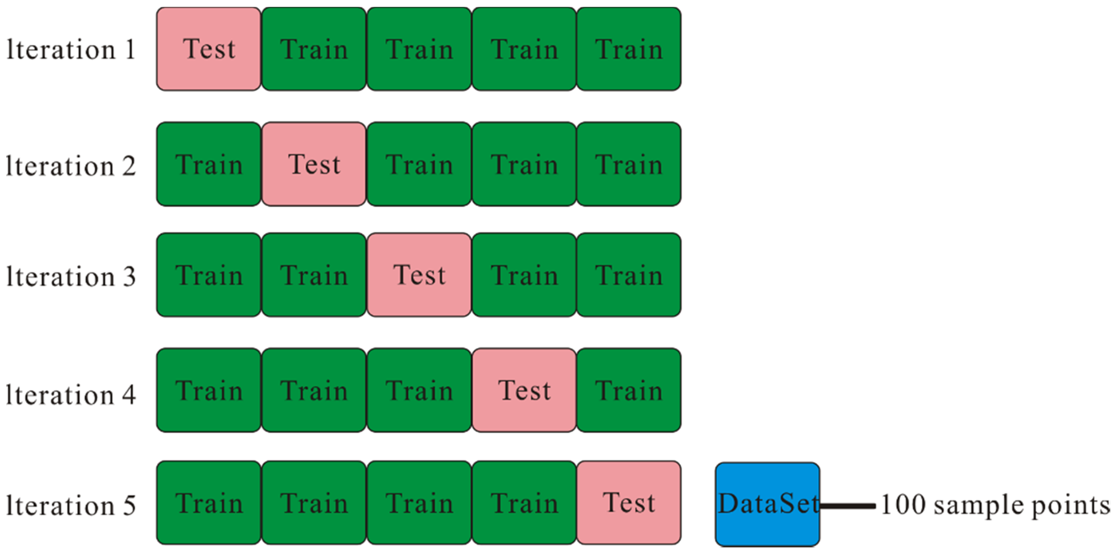
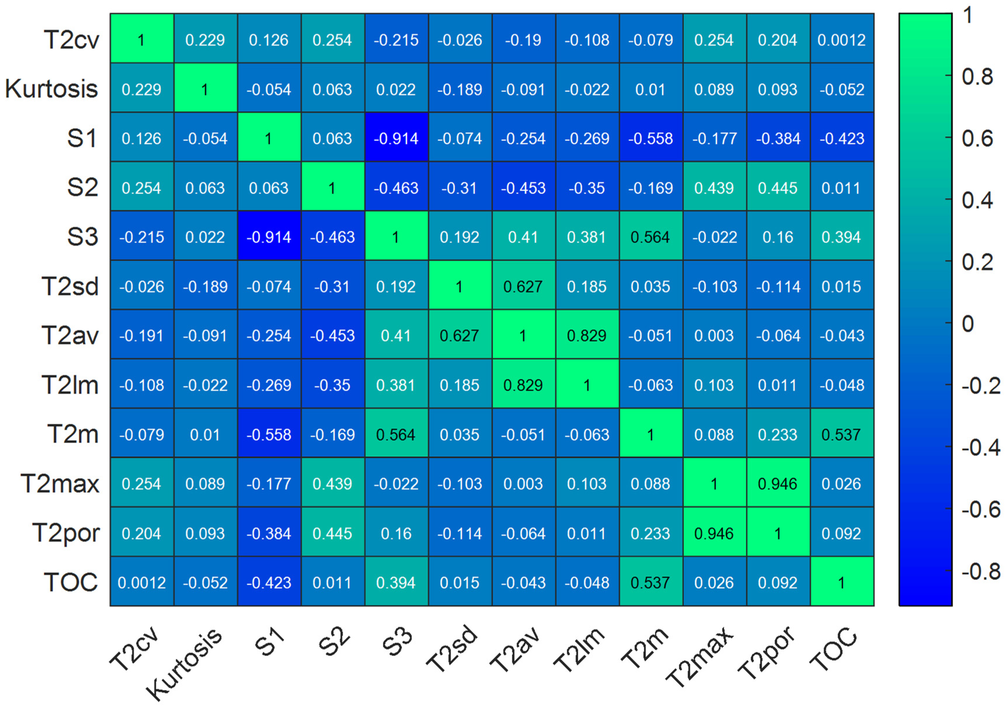
3.2. Data Preparation and Sensitivity Analysis

The experimental data in this paper are derived from the actual logging data of the Lianggaoshan Formation in well area x in Sichuan Basin, China. The response characteristics of logging curves and NMR logging represent the integrated response of stratigraphic information. This paper uses micro-parameters characterizing the pore structural features extracted from conventional logging curves and NMR T2 spectra to perform sensitivity analyses with the TOC content of the core analyses, eliminating the influence of multicollinearity. Thus, before developing the TOC prediction model, we utilized Pearson’s index to measure the correlation between each parameter and the core test TOC. Additionally, we opted to use the input eigenvectors of the TCN network model to enhance the stability of the TCN model. Equation (3) presents the formula for calculating the Pearson correlation coefficient.

$$P=\frac{N{\displaystyle {\sum }_{i=1}^N{x}_i}{y}_i-{\displaystyle {\sum }_{i=1}^N{x}_i}{\displaystyle {\sum }_{i=1}^N{y}_i}}{\sqrt{N{\displaystyle {\sum }_{i=1}^N{x}_i^2}-{({\displaystyle {\sum }_{i=1}^N{x}_i})}^2}\sqrt{N{\displaystyle {\sum }_{i=1}^N{y}_i^2}-{({\displaystyle {\sum }_{i=1}^N{y}_i})}^2}}$$

(3)

where x—individual logging parameters; y—core organic carbon content; i—serial number of each sample; N—total number of samples.

Figure 5 shows the Pearson correlation heat map between conventional logging curves and core test TOC content. It is not difficult to see that the correlation between core test TOC and the conventional logging curves is generally low, and most of the correlation between the logging curves and TOC is less than 0.1, which illustrates the characteristic of the shale reservoir in the study area to have a strong non-homogeneous nature. In this figure, relative to other logging parameters, acoustic logging (AC), density logging (DEN), and uranium (U) from gamma energy spectroscopy logging have relatively good correlation with the TOC content, so they can be used as the eigenvectors of the TCN network. Considering the effect of multicollinearity between parameters, the correlation between AC, DEN, and U needs to be considered. In the figure, it can be seen that Pearson’s parameter between the AC and DEN is −0.533, which is negatively correlated and has a small effect on multicollinearity, and the correlation between U and the AC and DEN curves is even lower, so there is no multicollinearity problem either. Figure 6 shows the correlation heatmap between each microporous structure parameter extracted from the NMR T2 spectrum and the laboratory test TOC, from which it can be seen that, relative to other parameters, the large pore fraction (S3) and the median value of the T2 spectrum (T2m) have a strong correlation with the TOC content, and their Pearson indices reach 0.4 and above. S3 represents the integral of the large pore fraction of the T2 spectrum, which can reflect the change characteristics of the pore structure of the rock. The median value is a statistical parameter in the porosity component of the T2 spectrum, reflecting the middle value of the porosity component of the T2 spectrum after sorting, which can characterize the pore throat characteristics of the reservoir to a certain extent, and there is a certain positive correlation with TOC. Similarly, the Pearson correlation coefficient between S3 and T2m is only 0.164, so there is no multicollinearity. So finally, the preferred input parameters in the NMR logging parameters are S3 and T2m, as the input features of the TCN model. To summarize, in this paper, a total of five feature vectors are preferred as the feature vectors of the TCN network in conventional logging, natural gamma energy spectroscopy and logging, and NMR logging, which are AC, DEN, U, S3 and T2m.

3.3. Model Construction

For any machine learning model, the hyperparameters are the key parameters that determine the model’s performance. The initial purpose of model training is to adjust these hyperparameters to obtain the weights and gradients that result in the smallest prediction error. This applies to both shallow machine learning algorithms and deep network structures. The selection of hyperparameters is based on changes in the loss function during training and the results of inverse fitting of the test set. This joint evaluation determines whether it is necessary to adjust hyperparameters such as the number of training rounds, batch size, and learning rate of the model. Once the hyperparameters have been determined, the optimal weights that minimize the prediction error can be obtained. In the subsequent prediction task, only the trained optimal weights should be used to load the inversion model between the logging parameters and the TOC content.

3.4. Data Standardization

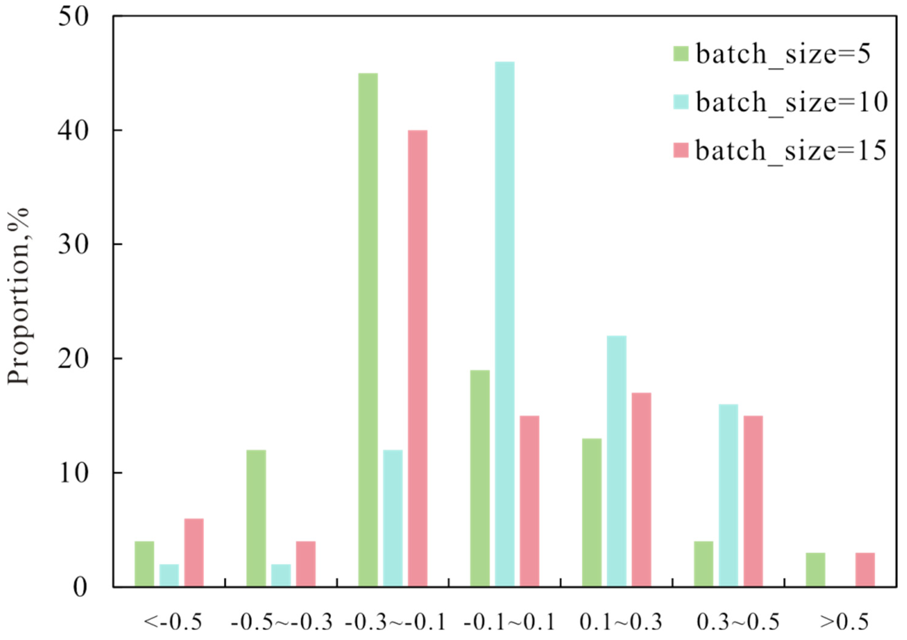
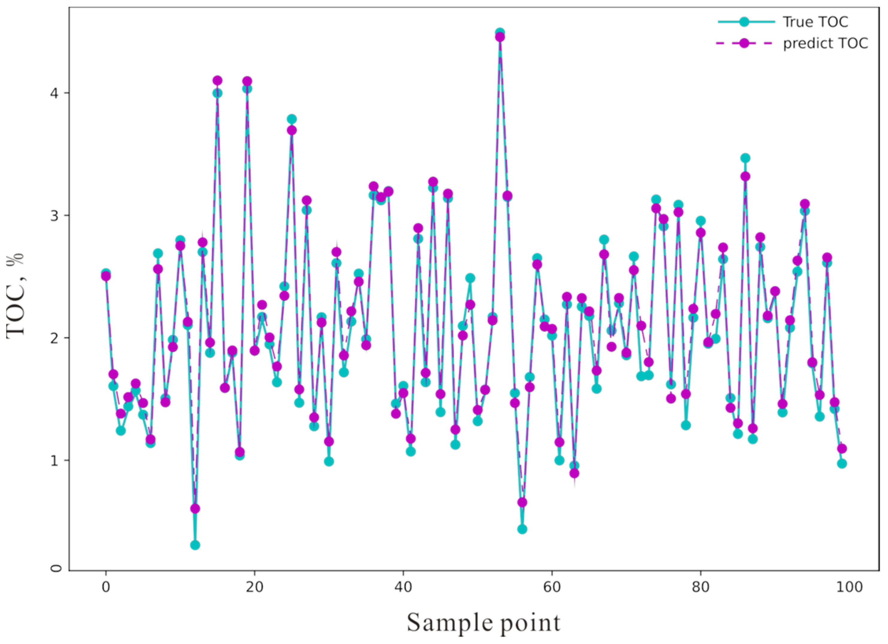
Before model training, it is important to mitigate prediction errors resulting from variations in logging parameters across different wells and layers. Additionally, the impact of outliers and extreme values should be eliminated. This paper adopts the z-score standardization processing method, which involves standardizing the feature vectors by their mean and standard deviation. This adjustment ensures that the feature vectors fall within a reasonable distribution range, leading to faster gradient drops during model training and ultimately resulting in a more effective trained model. The standardization expression is as follows:

$${\mathrm{y}}^{*}=\frac{y_i-\overline{y_i}}{s}$$

(4)

where $y_i$—input parameter; $\overline{y_i}$—mean value of this input parameter; s—standard deviation of this input parameter; $y^{*}$—data normalized for this input parameter.

3.5. Model Training

This paper presents logging data from the stratigraphy of the Lianggaoshan Formation in the Sichuan Basin, China. A total of 500 sets of data were collected for laboratory testing of TOC content. Compared to previous deep learning network models, the training sample size of 500 sets is relatively small. To make better use of this data for training, this paper employs the K-fold cross-validation method to determine the optimal hyperparameters of the TCN model. Cross-validation is primarily used in modeling applications. It involves taking most of the samples in a given modeling sample as training samples and using the remaining small samples for model validation. The K-fold cross-validation method divides the modeling sample into K equal parts, predicts each part in turn, and uses a few parts outside of its validation set for training. When all the samples have been traversed, it means that the model has been trained K times. Figure 7 presents the schematic diagram of the five-fold cross-validation. The 500 training samples are divided into five equal parts, each containing 100 sample points on average.

Using the mean square error as the evaluation index for the loss function, Figure 8a displays the change in the loss function curve after 100 training iterations. The model reaches the optimal gradient of the loss function during the 82nd training iteration, where the mean square error is at its minimum. However, the model exhibited overfitting when training was continued, so the number of training rounds was ultimately limited to 82 in this paper. Figure 8b illustrates the final training process of the model. The model has achieved convergence after 82 training rounds. After 82 rounds of iterative training, the Nadam optimizer is used to optimize the model, and the optimal combination of TCN model parameters is selected: the learning rate is 0.01, the number of hidden layers is 2, the number of neurons in each layer is 64, and the number of channels as well as other parameters are set as default parameters. Meanwhile, the L2 regularization technique is used to prevent overfitting, and the activation function uses the ReLU function to extract the eigenvector features to improve training efficiency and make the model more robust. During the training process, the author discovered that the sample batch size (number of data samples captured in a single training session) has a significant impact on the training results. Therefore, we conducted separate experiments on batch size, with a total of three groups of experiments. Due to the small sample size, we set the batch sizes to 5, 10, and 15, respectively, while keeping the other network parameters consistent. The training was carried out in this order. Finally, the error results for the three sets of experimental training are obtained. Figure 9 shows the histograms of the error distributions for the three sets of experiments. The horizontal axis represents the error distribution, and the vertical axis represents the percentage of the error distribution. It is evident that for a batch size of 10, the majority of errors fall within the range of −0.1 to 0.1, which represents 45% of the 100 validation sample sets. This suggests that the error rate is minimal. The error distribution shows the highest percentage between −0.3 and −0.1 for batch sizes of 5 and 15, which is approximately 40%. This suggests that the prediction results are generally smaller than the actual TOC. After conducting three experiments with different batch sizes, this paper concludes that the optimal batch size is 10. After determining the optimal combination of parameters, the model is set to train with the optimal parameters to obtain the optimal weights. Figure 10 displays the results of the optimal parameter TCN model predicting 100 samples in the validation set. The predicted TOC change trend is relatively consistent with the actual trend, except for a few instances where the predicted values are significantly higher or lower. This result confirms that the optimal parameters obtained from the training are correct. It also shows that the optimal parameter TCN model can better map the training set feature vectors and labels. Therefore, the trained weights were saved for the task of predicting the entire well section in the study area.

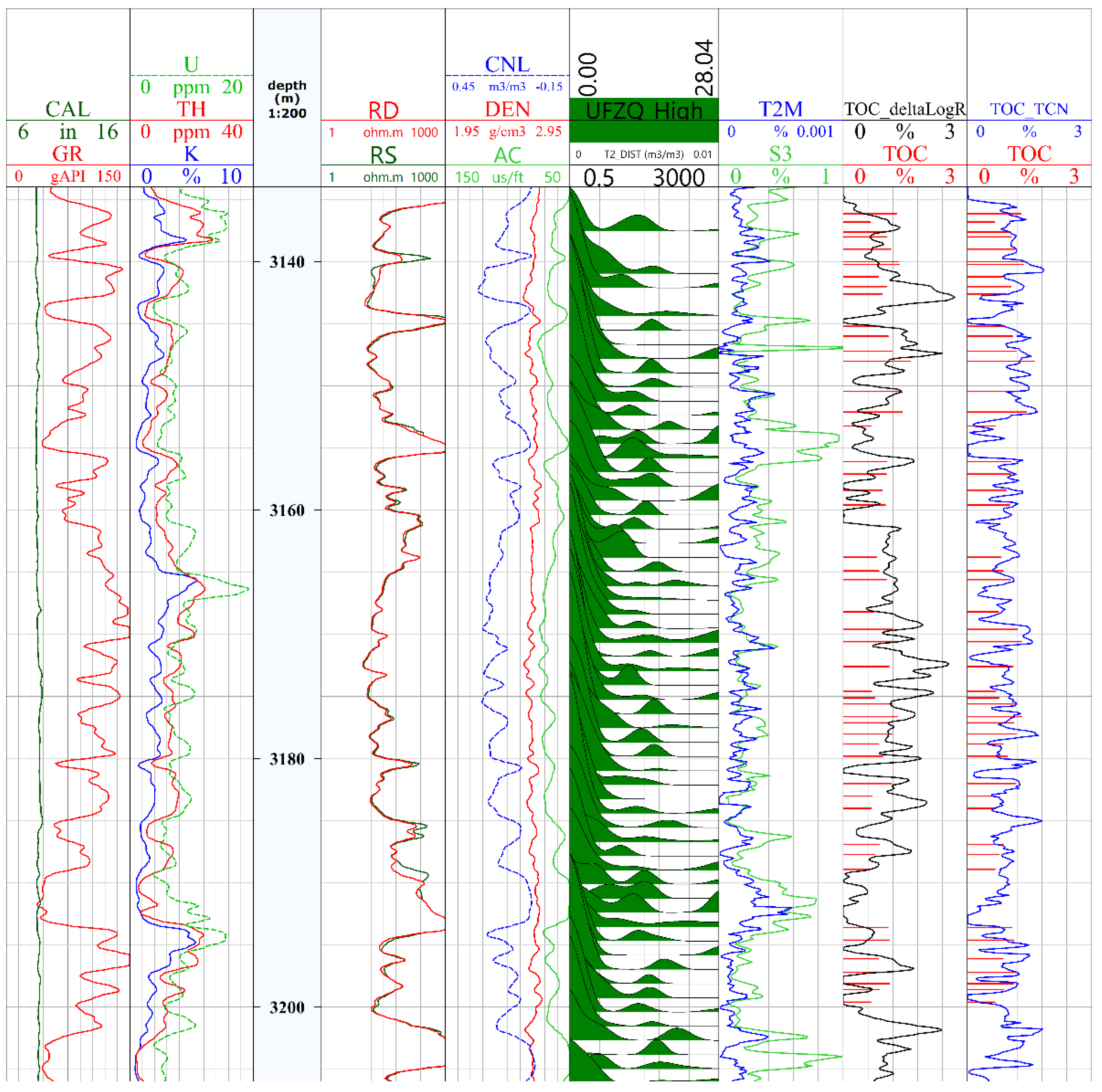
4. Methodological Applications

The saved weights were loaded into the TCN model framework to predict the total organic carbon content of a well section in the study block. At the same time, the well section was evaluated for total organic carbon content using the traditional ΔLogR method as well, as a way to compare the results. The ΔLogR method primarily uses the magnitude of the resistivity curve and the acoustic time difference curve, respectively, versus the baseline to calculate ΔLogR, and then uses ΔLogR and the maturity parameter (LOM) to establish a linear relationship with the TOC. Figure 11 illustrates the scatter plot between the TOC predicted by the two methods and the TOC from the core tests, and it is clear that the TCN model predictions are more closely aligned with the laboratory results, and that the TCN exhibits strong robustness both in the TOC intervals and in the relatively high TOC intervals. The traditional ΔLogR method is too sensitive to logging curves and strongly influenced by the baseline value of the stacked curves to effectively characterize the TOC content of shale. Figure 12 shows the results of TOC prediction for a well section in the study area, with lane 8 showing the TOC profile calculated by the ΔLogR model and lane 9 showing the TOC profile obtained from the TCN model prediction. The comparison indicates that the TCN model outperforms the LogR model in terms of prediction accuracy. The TCN model takes multiple logging parameters as inputs and is not affected by transfer errors caused by multiple parameters, which results in a strong fitting ability to the input parameters. Particularly in the depth section between 3165 and 3175 m, the logging response parameters underwent significant changes. However, the final predicted TOC curves remained stable, indicating the TCN model’s robustness against overfitting. Meanwhile, in the depth section where the changing of total organic carbon content is more blocky, the TCN model can accurately predict the change trend of TOC content in the longitudinal direction because of its strong feature extraction ability and time series processing ability.

Table 1. Error statistics of TOC prediction results.

Model	Absolute Error	Relative Error
ΔLogR	0.49	0.53
TCN	0.13	0.14

counts the error results of the two models when predicting TOC, and it can be seen that the TCN model reduces the absolute error from 0.49 to 0.13 and the relative error from 0.53 to 0.14 compared to the traditional model. In summary, the TCN prediction model has a higher prediction accuracy, and at the same time, it can still maintain good results in the depth section where the stratigraphy changes drastically, reflecting a good generalization ability, which is helpful for the evaluation of shale total organic carbon content.

5. Conclusions

The prediction of TOC content is an important part of the logging evaluation of hydrocarbon source rock quality. In this paper, conventional logging data, NMR logging data, and core experiment analysis data are combined. To eliminate the influence of multicollinearity, this paper uses the Pearson correlation coefficient, specifies the five parameters AC, DEN, U, S3, and T2m as feature vectors, and uses the core analysis TOC as label vectors. In this paper, a TCN network was established, a TOC logging evaluation framework was constructed, and an optimal TCN network model was constructed by using five-fold cross-validation to train 500 sets of data in the study area, determining the optimal number of training rounds to be 82 rounds and the optimal batch size to be 10. Finally, in this paper, the TOC prediction problem is viewed as a time series problem, and the feature vectors of a certain segment depth are used to predict the TOC content at a certain depth point. For the first time, the time series prediction model is applied to the task of TOC content prediction, and the prediction effect is better compared with the ΔLogR traditional model, the absolute error is reduced from 0.49 to 0.13, and the relative error is reduced from 0.53 to 0.14, which can provide a technical means for intelligent shale reservoir parameter prediction.

References

1. Bi, C. Study on Prediction Method of TOC Content Brittleness Index of Shale Reservoir. Ph.D. Thesis, China University of Geosciences (Beijing), Beijing, China, 2021. [Google Scholar]
2. Yuan, C.; Zhou, C.; Hu, S.; Chen, X.; Dou, Y. Summary on well logging evaluation method of total organic carbon content in formation. Prog. Geophys. 2014, 29, 2831–2837. [Google Scholar]
3. Zhu, L. An improved method for evaluating the TOC content of a shale formation using the dual-difference ΔlogR method. Mar. Pet. Geol. 2019, 102, 800–816. [Google Scholar] [CrossRef]
4. Huo, Q.; Zeng, H.-S.; Fu, L.; Ren, Z. The Advance of ΔlgR Method and Its Application in Songliao Basin. J. Jilin Univ. (Earth Sci. Ed.) 2011, 41, 586–591. [Google Scholar]
5. Passey, Q.R.; Creaney, S.; Kulla, J.B. A practical model for organic richness from porosity and resistivity logs. AAPG Bull. 1990, 74, 1777–1794. [Google Scholar]
6. Huang, S.; Liu, W.; Dai, H.; Wang, X.; Sun, L.; Liu, D. Log Evaluation on the TOC of Continental Source Rocks based on Variable Coefficient ΔlgR Model. Well Logging Technol. 2019, 43, 519–523. [Google Scholar]
7. Zhou, C.; Wang, L.; Su, S.; Xue, K.; Wang, Q. Research on organic carbon content logging evaluation method based on ΛLogR-GR method: Case study from study Mao-1 in Southeastern Sichuan Basin. Nat. Gas Geosci. 2023, 35, 542–552. [Google Scholar]
8. Jacobi, D.; Gladkikh, M.; Lecompte, B. Integrated petrophysical evaluation of shale gas reservoirs. In Proceedings of the Canadian International Petroleum Conference, SPE Gas Technology Symposium Joint Conference, Calgary, AB, Canada, 16–19 June 2008. [Google Scholar]
9. Lu, P.; Mao, X.; Zhang, F. Prediction of organic carbon content in Lunpola Basin by neural network method. Prog. Geophys. 2021, 36, 230–236. [Google Scholar]
10. Zhu, L.; Zhang, C.; Wei, Y.; Guo, C.; Zhou, X.; Chen, Y. The Method for TOC Content Evaluation in Shale Reservoirs Based on Improved Rain Forest Fuzzy Neural Network Model. Geol. J. China Univ. 2016, 22, 716–726. [Google Scholar]
11. Zhu, L.; Zhang, C.; Zhang, C.; Zhang, Z.; Zhou, X.; Liu, W.; Zhu, B. A new and reliable Dual model- and data-driven TOC prediction concept: A TOC logging evaluation method using multiple overlapping methods integrated with semi-supervised deep learning. J. Pet. Sci. Eng. 2020, 188, 106944. [Google Scholar] [CrossRef]
12. Yang, W.; Zhang, C.; Yang, M. Permeability logging evaluation of carbonate reservoirs in Oilfield H of Iraq in the Middle East based on long short-term memory recurrent neural network. Pet. Geol. Oilfield Dev. Daqing 2022, 41, 126–133. [Google Scholar]
13. Zhou, X.; Zhang, Z.; Zhu, L.; Zhang, C. A new method for high-precision fluid identification in bidirectional long short-term memory network. J. China Univ. Pet. (Ed. Nat. Sci.) 2021, 45, 69–76. [Google Scholar]
14. Lea, C.; Flynn, M.D.; Vidal, R.; Reiter, A.; Hager, G.D. Temporal Convolutional Networks for Action Segmentation and Detection. In Proceedings of the IEEE Conference on Computer Vision and Pattern Recognition (CVPR), Las Vegas, NV, USA, 27–30 June 2016. [Google Scholar]
15. Shekhamer, E.; Long, J.; Darrell, T. Fully convolutional networks for semantic segmentation. IEEE Trans. Pattern Anal. Mach. Intell. 2017, 39, 640–651. [Google Scholar] [CrossRef] [PubMed]
16. He, K.M.; Zhang, X.Y.; Ren, S.Q. Deep residual learning for image recognition. In Proceedings of the 2016 IEEE Conference on computer Vision and Pattern Recognition (CVPR), Las Vegas, NV, USA, 27–30 June 2016; pp. 770–778. [Google Scholar]
17. Bai, S.; Cheng, D.; Wan, J. Quantitative characterization of sandstone NMR T2 spectrum. Acta Pet. Sin. 2013, 34, 366–371. [Google Scholar]
18. Yang, W.; Zhang, C.; Shi, X.; Cui, Y.; Zhang, Z. Reconstruction of LWD-NMR T2 water spectrum and fluid recognition based on microscopic pore structure constraints. Geoenergy Sci. Eng. 2023, 221, 211386. [Google Scholar] [CrossRef]
Figure 1. Schematic diagram of the basic structure of TCN.
Processes 12 00610 g001
Figure 4. Schematic representation of the microscopic parameters of the NMR T2 map.
Processes 12 00610 g004
Figure 5. Thermogram of correlation between conventional logging profiles and core test TOC content.
Processes 12 00610 g005
Figure 6. Heat map of correlation between NMR logging parameters and tested TOC content.
Processes 12 00610 g006
Figure 7. Schematic diagram of five-fold cross-validation.
Processes 12 00610 g007
Figure 8. (a) Model loss function variation curve for 100 rounds of training; (b) model loss function variation curve for 82 rounds of training.
Processes 12 00610 g008
Figure 9. Distribution of prediction errors for different sample batch sizes.
Processes 12 00610 g009
Figure 10. Optimal-parameter-combination TCN model validation set prediction results.
Processes 12 00610 g010
Figure 11. Scatter plot of predicted TOC and real TOC.
Processes 12 00610 g011
Figure 12. Map of predicted results of a stratigraphic section in well X.
Processes 12 00610 g012