A Series Arc Fault Diagnosis Method Based on an Extreme Learning Machine Model

Abstract

In this study, we address the critical issue of accurately detecting series AC arc faults, which are often challenging to identify due to their small fault currents and can lead to devastating electrical fires. We propose an intelligent diagnosis method based on the extreme learning machine (ELM) model to enhance detection accuracy and real-time monitoring capabilities. Our approach involves collecting high-frequency current signals from 23 types of loads using a self-developed AC series arc fault data acquisition device. We then extract 14 features from both the time and frequency domains as candidates for arc fault diagnosis, employing a random forest to select the most significantly changed features. Finally, we design an ELM classifier for series arc fault diagnosis, achieving an identification accuracy of 99.00% ± 0.26%. Compared to existing series arc fault diagnosis methods, our ELM-based method demonstrates superior recognition performance. This study contributes to the field by providing a more accurate and efficient diagnostic tool for series AC arc faults, with broad implications for electrical safety and fire prevention.

1. Introduction

While electricity provides convenience for our daily lives, it also brings many safety risks. The household power consumption system is the most widely distributed load in the power system, and its safety and stability are closely related to the life and property of the people. According to the 2021 national fire rescue team receiving and handling police and fire situation report data released by the Fire Rescue Bureau of the Ministry of Emergency Management, there were 7,408,000 fires, 1987 deaths, 2225 injured people, and direct property losses of 6.75 billion yuan in 2021. Compared with 2020, the number of injuries and losses increased by 9.7%, 24.1%, and 28.4%, respectively, and the number of deaths decreased by 4.8% [1]. Electrical fires are still the main causes of major fire accidents, accounting for 28.4% of the total number of fire accidents in China. Nearly one-third of large fires are caused by electrical factors, the majority being electrical line faults, which account for nearly 80% of the total number of electrical fires [2].

As shown in Figure 1, there are three types of arc faults: series arc faults, parallel arc faults, and grounding arc faults. Parallel arc faults and grounding arc faults generate large currents that are easily identified by circuit breakers. When a series arc fault occurs, the current in the circuit is small, its characteristics change with different loads, and the detection difficulty is high. Such faults have become the main causes of fire, so to realize the accurate detection of series arc faults has important social significance and broad market prospects [3,4].

From the perspective of fault arc detection parameters and detection algorithms, most current arc fault detection methods at home and abroad include those based on mathematical modeling, those based on accompanying physical signals, and those based on electrical signals [5,6,7,8,9]. Since the arc fault current has nothing to do with the location of the arc, measuring the high-frequency current signal and voltage waveform of the bus bar has become the most common method to detect an arc fault. A digital signal processing method is used to extract the fault features, and the extracted features are used as the input of the classifier model to detect the arc fault [10,11,12].

In recent years, there has been a significant focus on the diagnosis of series AC arc faults in electrical systems, with particular emphasis on improving detection accuracy and real-time monitoring capabilities. Guo et al. used a five-layer wavelet transform to decompose the raw signal and established an electric arc fault detection model based on particle swarm optimization and grid search optimization [13]. Han et al. [14] presented a method for series arc fault detection based on category identification and artificial neural networks. A wavelet transform was conducted to extract time and frequency domain features as input to an artificial neural network, and thus establish a BP neural network optimized by three different loads. Li et al. exploited the energy entropy and sample entropy of intrinsic mode functions of variational mode decomposition by the raw signal, establishing an arc fault diagnosis model of the optimized limit learning machine based on a sparrow search algorithm [15]. Zhang et al. presented a method that enhances data and employs an adaptive asymmetric CNN for series AC arc fault diagnosis, highlighting the potential of asymmetric networks in improving diagnostic accuracy [16]. Wang et al. utilized a fully connected neural network to analyze hybrid time and frequency features for series AC arc fault diagnosis, underlining the effectiveness of neural networks in processing complex fault signatures [17]. In summary, the research on these issues provides technical insights into the identification of series arc faults while facing the following challenges:

(1)

Noise susceptibility: Many detection algorithms are sensitive to electrical noise and circuit disturbances, which can lead to misdetections or false alarms;

(2)

Model interpretability: Advanced neural network models often lack interpretability, making it difficult to understand the reasoning behind their predictions;

(3)

Complexity and real-time capability: Deep learning models, while effective, can be computationally intensive and may not meet the real-time requirements of some applications, e.g., circuit breakers.

Therefore, we propose a method based on an extreme learning machine (ELM) to detect series arc faults. ELMs have garnered significant attention for their applications in both classification and regression tasks. Characterized as a single hidden layer feedforward neural network, the ELM stands out due to its high accuracy and low complexity. It boasts rapid learning speeds and robust generalization capabilities, which have led to the extensive adoption of ELMs in data classification across diverse disciplines [18]. In this study, the ELM was selected to design the classifier for series arc fault detection. First, we built a series arc fault experimental system, carried out the arc fault diagnosis experiment under different working conditions, and collected the high-frequency current signal of the fault arc. Second, the eight time-domain features and six frequency-domain features of the fault current signal were extracted as arc fault features, and the extracted features were trained using random forest (RF). The design of the limit learning machine arc fault classifier to realize the fault arc diagnosis and its recognition performance were evaluated.

2. Experimental Data

The experimental data presented in this paper were collected using a fabricated low-voltage AC series arc fault data acquisition device suitable for the 220V power supply network. The experimental equipment is shown in Figure 2. Figure 2a shows the composition of the experimental equipment, which includes a power supply, arc generator, current acquisition module, and load. The arc generator connects the load and the current acquisition module, generating the arc when working. The current acquisition module generates the load current signal. The HC-08 Bluetooth module is connected to the LabVIEW2020 to collect the load current data, and the high-frequency current transformer connected to the current acquisition module is connected to the load fire wire to obtain the load working current. Figure 2b shows the structural diagram of the current collection module, which consists of an input power supply, a current conversion module, a high-frequency current sensor, and a low-frequency current sensor. The power supply is 220AC, and the core of the current conversion module is the Stm32F407 microcontroller of STMicroelectronics, which is responsible for signal acquisition and wireless transmission. The high-frequency current sensor has a high-frequency cutoff frequency of 10 KHz, and the low-frequency current sensor has a low-frequency cutoff frequency of 1 KHz. The high-frequency current is used for arc identification, and the low-frequency current is used to calculate the magnitude of the current in the circuit. The signal ADC is 12-bit, and the Bluetooth communication baud rate is 1,382,400 bps.

Common household low-voltage AC appliances were used as the experimental load, and the names of the electrical appliances, load types, and other information are shown in

Table 1. Load information.

Order Number	Load Name	Operate Mode	Load Type
1	Electric warm wind	cold air blast	Inductive type
		low-grade fever	Inductive resistance type
		ardent fever
2	hair drier	cold air I file	Inductive type
		cold wind II file	Inductive type
		hot air low temperature I file	Inductive resistance type
		hot air low temperature II file
		hot air high temperature I file
		hot air high temperature II file
3	electric screwdriver	await the opportune moment	Switch power type
		idling	Switch power supply type + inductance
4	teakettle	heat up water	Resistance type
5	jinbao electric screwdriver 1	await the opportune moment	Switch power type
		idling	Switch power supply type + inductance
6	jinbao electric screwdriver 2	await the opportune moment	Switch power type
		idling	Switch power supply type + inductance
7	double row of lights	lighting	Resistance type
8	desk lamp	natural light	Resistance type
		white light
		warm light
9	cloth lamp	lighting	Resistance type
10	bedlamp	low bright	Switch power supply type + resistance
		highlight
11	LED tape lights	lighting	Switch power supply type + resistance
12	Op LED light	lighting	Switch power supply type + resistance
13	bull lamp	lighting	Switch power supply type + resistance
14	halogen lamp	lighting	Resistance type
15	vacuum cleaner	low-end	Inductive type
		top grade
16	electrodrill	revolve	Switch power supply type + inductance
		hammer turn
17	cutting machine	idling	Switch power supply type + inductance
18	electric fan	1 file	Resistance type
		2 file
		3 file
19	microwave oven	Low fire	Inductive type
20	electromagnetic oven	120W	Inductive type
		1000W
		2100W
21	humidifier	low-end	Resistance type
		top grade
22	refrigerator	work	Inductive type
23	indicator	work	Switch power supply type + resistance

. There are 23 types of loads selected, including resistance (R), inductive (I), inductive resistance (RI), and switch power supply (SW). During the experiment, first, collect the current signal of the load and then collect the current signal of the arc generator in the arc pulling state.

For the 23 types of loads shown in Table 1, we collected experimental data from 43 gear positions under normal and arcing conditions, with 40 sets of data collected for the normal state of each gear position and 40 sets of data collected for the arcing state. Therefore, there are a total of 43 × 2 × 40 = 3440 sets of data. The signal sampling frequency is 35.7 kHz, and the length of each set of data is 120 ms.

The waveform of the high-frequency current signal collected is shown in Figure 3. In order to increase the data accuracy and the number of model training samples, five groups of tests were carried out in each type of test scheme.

3. Algorithm Principle

3.1. The Proposed Method Process

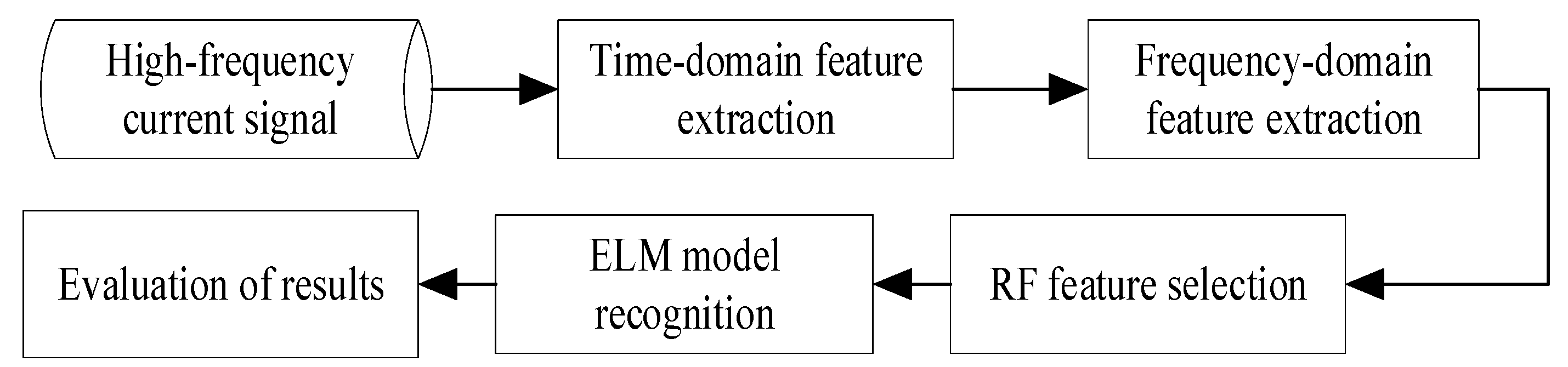
The AC arc fault identification process is shown in Figure 4. The high-frequency current signal is recorded by our developed device. Next, some time-domain and frequency-domain features are extracted as arc fault features, and the RF is employed in arc fault detection by evaluating whether these features have significantly changed. Moreover, the ELM classifier is trained and tested by the selected features. Finally, some indexes, e.g., kappa coefficient (KC), specificity, sensitivity, and accuracy, are engaged to evaluate the performance of the ELM model.

3.2. Feature Extraction

In order to ensure that the designed limit learning machine classifier can achieve high identification accuracy, it is necessary to extract the arc fault features that can truly reflect the arc characteristics as the input of the limit learning machine model, and the extracted fault arc features need to be able to effectively distinguish the normal working state and the arc fault state.

In this paper, we extract eight frequency-domain features and 6 time-domain features as inputs to the limit learning machine classifier. The extracted time-domain features include the standard deviation, effective value, peak factor, pulse factor, waveform factor, margin factor, cliff degree factor, and skewness factor. After normalizing the collected current signal, the high-frequency current signal is FFT-transformed to calculate the first five harmonics. The extracted frequency domain features include the mean spectrum, spectrum standard deviation, fundamental wave component ratio, relative fundamental wave component ratio, relative third harmonic component ratio, and relative fifth harmonic component ratio.

3.3. Feature Selection Based on Random Forests

In the domain of fault diagnosis, the application of random forests for feature selection is a pivotal technique. Random forests (RFs) operate by leveraging an ensemble of decision trees for both the training and prediction of samples. Their most notable strength lies in their capacity to gauge the significance of individual features. Consequently, feature selection can be tailored to various load types, allowing for the identification of the most suitable feature subset. Central to this process is the Gini impurity, a metric that quantifies the probability of misclassifying new instances of random variables.

$$I_{\mathrm{G}} (f)={\displaystyle \sum _1^m{f}_i (1-f_i)}={\displaystyle \sum _1^m{f}_i}-{\displaystyle \sum _1^m{f}_i^2}=1-{\displaystyle \sum _1^m{f}_i^2}$$

(1)

where, represents the proportion of a class of samples that belong to that class. Consider the case of arc fault detection, where the sample set is divided into two distinct categories: normal and fault. Consequently, we have m = 2. Within this framework, f₁ signifies the proportion of samples that are normal, while f₂ denotes the proportion of samples that are faulty.

$$\Delta I_G^n(f)=I_{G\text{-}NE}(f)-I_{G\text{-}E}(f)$$

(2)

The Gini impurity associated with a particular feature within a decision tree is computed. Analogously, the Gini impurity for the decision tree excluding this feature is also determined.

The difference between these two values quantifies the reduction in Gini impurity attributable to the feature in question within the decision tree. To assess the overall impact of the feature, the Gini impurity reduction is calculated across all decision trees, and the average reduction, termed the mean decrease in impurity (MDI), is then derived.

$$MDI={\displaystyle \frac{{\displaystyle \sum _1^N\Delta I_G^n (f)}}{N}}$$

(3)

The MDI serves as a quantitative metric for evaluating the influence of individual features on the random forest’s performance. A higher MDI value indicates a greater contribution of the feature to classification accuracy, thereby enhancing the stability of the random forest model.

3.4. Series Arc Fault Diagnosis Technology Based on the Limit Learning Machine

The extreme learning machine (ELM) is a three-layer feedforward neural network that contains only one hidden layer. In ELM, the hidden layer deviation and connection weights between each layer are both automatically generated, and the simple structure makes the ELM easy to build, gives it a faster learning speed than traditional neural networks, and allows it to use fewer computational resources.

The extreme learning machine is an effective and simple learning method. The random generation of the hidden nodes of the ELM improves its learning speed. Considering its advantages—its high learning efficiency, simple concept, and good generalization ability—the ELM is selected as the classifier model for arc fault diagnosis [19].

Order [x_i,t_i] (i ∈ 1, 2, …, N) represents N training samples. The ith training sample true label matrix, xi = [x_i1, x_i2, …, x_in]^T ∈ Rⁿ, is ti = [t_i1, t_i2, …, t_im]^T ∈ R^m. Define n as the count of neurons in the input layer, which corresponds to the number of features within each sample. Let m represent the number of neurons in the output layer, mirroring the number of classes present in the dataset. Furthermore, denote L as the number of neurons in the hidden layer. The matrix of input weights can be formulated as U = [u₁, u₂, …, u_L]^T ∈ R^L×n, where each ui = [u_i1, u_i2, …, u_in]^T ∈ Rⁿ, for i ∈ {1, 2, …, L}. The bias vector for the hidden layer is given by b = [b₁, b₂, …, b_L]^T ∈ R^L. The output of the ith training sample at the hidden layer is detailed in Equation (4).

$$h(xi)=g(Uxi+b)$$

(4)

Among these, g(.) for the activation function, and the ‘sigmoid’ function are employed in this study. The hidden layer output matrix, composed of all the training samples, is marked as H in Formula (5), and the dimension is n × L.

$$H=\left[\begin{array}{c}h(x_1)\\ \dots \\ h(x_N)\end{array}\right]=\left[\begin{array}{c}g(u_1{x}_1+b_1)\dots g(u_L{x}_1+b_L) \\ \dots \\ g(u_1{x}_N+b_1)\dots g(u_L{x}_N+b_L)\end{array}\right]$$

(5)

Consider β_ij as the synaptic weight connecting the hidden layer neuron Bi to the output neuron Oj. The matrix representing the output weights is presented in Equation (6).

$$\beta =\left[{\beta }_1,\dots ,{\beta }_m\right]=\left[\begin{array}{c}{\beta }_{11}\dots {\beta }_{1m}\\ \dots \\ {\beta }_{L1}\dots {\beta }_{Lm}\end{array}\right]\in R^{L\times m}$$

(6)

The optimization function of the ELM is shown in Formulas (7) and (8):

Minimality:

$${\displaystyle \frac{1}{2}}\Vert \beta {\Vert }^2+C{\displaystyle \frac{1}{2}}{\displaystyle \sum _{i=1}^N{‖\xi i‖}^2}$$

(7)

$$h(xi)\beta =t_i^T-{\xi }_i^T, i=1,2,\dots ,N$$

(8)

where ξi = [ξ_i1, ξ_i2, …, ξ_in]^T is the vector of the training error composition of sample x_i on the m output nodes.

The ELM algorithm was selected to design the classifier for series arc fault detection, using 1000 sets of data in the dataset as the training set and the 2 remaining 378 sets as the test set, normalized to the dataset. Using the MATLAB2023 neural network toolbox, we can establish the limit learning machine classifier in MATLAB and train the limit learning machine classifier model using the function ‘elmtrain(P,T,N,TF,TYPE)’. P is the feature in the training set that acts as the input to the model, T is the label in the output of the model in the training set, N is the number of neurons in the hidden layer, set to 30 by tail and test, TF is the category of the hidden layer activation function, select ‘tansig’ function, TYPE is the application type of ELM, and the value of 1 indicates the classification. The function ‘elmpredict(P,IW,B,LW,TF,TYPE)’ is used to conduct the arc fault diagnosis of the trained ELM model in the test set. P is the feature of the test set that acts as the model input, IW is the connection weight between the input layer and the hidden layer, B is the threshold of the hidden layer, and LW is the connection weight of the hidden layer and the output layer.

3.5. Classification Performance Evaluation Index of the Extreme Learning Machine Classifier

At present, the common classifier classification performance measures include R2, RMSE, MAE, VAF, a20-index [20], double-fault [21], kappa [22], margin measure [23], sensitivity, specificity, accuracy, and other [24]. For the purposes of this study, we identified a set of metrics to gauge the efficacy of the classifier based on the extreme learning machine (ELM). These metrics are employed to validate the classification precision of the developed ELM model. The chosen performance indicators include specificity (Sp), sensitivity (Se), accuracy (Ac), and the kappa coefficient (KC), which collectively serve to assess the classification capabilities of the ELM classifier.

In assessing the diagnostic results for arc fault states, specificity (Sp) quantifies the proportion of non-arc states correctly identified as such, also referred to as the true negative rate. A higher specificity value denotes greater accuracy in distinguishing non-arc states. The formula for calculating specificity is provided in Equation (9).

$$Sp={\displaystyle \frac{TN}{FP+TN}}\times 100\%$$

(9)

Sensitivity (Se), also termed the true positive rate, measures the proportion of actual arc states correctly identified out of the total number of arc states. A higher sensitivity indicates a more accurate detection of arc states by the model. The calculation for sensitivity is delineated in Equation (10), reflecting the model’s capacity to identify positive instances.

$$Se={\displaystyle \frac{TP}{TP+FN}}\times 100\%$$

(10)

Accuracy (Ac) quantifies the proportion of correctly classified samples, including both normal operating states and arc fault states, relative to the total sample size. A higher accuracy value signifies a greater rate of correct identification. The formula for determining accuracy is presented in Equation (11).

$$Ac={\displaystyle \frac{TP+TN}{TP+FP+FN+TN}}\times 100\%$$

(11)

In the context of classification outcomes, TP, FP, FN, and TN denote true positives, false positives, false negatives, and true negatives, respectively. Specifically, TP represents the count of instances correctly identified as normal states, FP indicates the number of arc states incorrectly classified as normal, FN is the count of normal states misclassified as arc states, and TN denotes the number of arc states accurately identified as such.

The kappa coefficient (KC) is employed to assess the agreement between predicted and actual classification outcomes, thereby evaluating the classification efficacy of the model. It quantifies the degree to which the model’s predictions align with the true classifications. The computation of the kappa coefficient is detailed in Equations (12)–(14).

$$KC={\displaystyle \frac{p_0-p_e}{1-p_e}}$$

(12)

$$p_0={\displaystyle \frac{{\displaystyle \sum _{t=1}^r{q}_{tt}}}{m}}$$

(13)

$$p_e={\displaystyle \frac{{\displaystyle \sum _{t=1}^r(q_{t+}\times q_{+t}})}{m^2}}$$

(14)

where $p_0$ is the ratio of the sum of diagonal elements of the entire elements and the confusion matrix $p_e$ is the ratio of the sum of the actual and the predicted number of samples, r is the number of rows of the confusion matrix, $q_{t+}$ is the sum of all elements in row t, and $q_{+t}$ is the sum of all elements in column t.

The value of KC is within [0, 1], and the closer the KC value of the classifier is to 1, the higher the classification accuracy of the classifier.

${KC}_t$ is the kappa coefficient corresponding to each classification result, and the calculation formula is shown in (15)–(18):

$$K{C}_t={\displaystyle \frac{P_{tt}-P_{t+}{P}_{+t}}{P_{+t}-P_{t+}{P}_{+t}}}$$

(15)

$$P_{tt}={\displaystyle \frac{q_{tt}}{m}}$$

(16)

$$P_{\mathrm{t}+}={\displaystyle \frac{q_{t+}}{m}}$$

(17)

$$P_{+t}={\displaystyle \frac{q_{+t}}{m}}$$

(18)

4. Results

In this study, we select the 14 arc fault features based on the feature importance ranking of random forest. The results of the feature selection are shown in Figure 5, and the standard deviation, waveform factor, cliff degree factor, and skewed degree factor of the high-frequency current are selected as the input of the arc fault diagnosis classifier of the ELM.

The 3440 sample states are predicted, with the corresponding labels set for different working states of the typical load data set; label 2 is the arc state and label 1 is the normal working state.

Furthermore, in order to compare our method with existing common methods, we designed probabilistic neural network (PNN) and back propagation neural network (BPNN) classifiers, and trained them using experimental data. The PNN consists of two layers in total. The first layer employs RBF (radial basis function) as the transfer function, and the second layer is a competitive layer that outputs the classification results. The transmission speed of the RBF is 0.02. The BPNN has a total of three layers, namely, the input layer, the hidden layer, and the output layer, with 20 neurons in the hidden layer. The transfer functions for the hidden layer and the output layer are ‘tansig’ and ‘purelin’, respectively.

The BPNN, PNN, and ELM were employed to detect AC arc faults. After feature normalization, 1000 sets of data from 3440 sets of data under different working conditions were randomly selected as the training set, and the rest were used as the test set for fault arc diagnosis. We verified that the training constants used across different models and algorithms were selected based on a grid search methodology, ensuring that they were optimal and fair for comparison. The initial weights for all neural network models were randomized using the same seed to maintain consistency. To further strengthen the fairness of the comparison, we implemented k-fold cross-validation for all models. This ensures that the models are evaluated on an equal number of data points and under similar conditions. The BPNN and feature extraction method of Wu et al. [25] were employed in this study for comparison. Meanwhile, the PNN-based method proposed by Jiang et al. was also used for comparison [26].

The classification performance was evaluated by four indicators: specificity (Sp), sensitivity (Se), accuracy (Ac), and kappa coefficient (KC). The results of selecting different classifiers are shown in

Table 2. Results of performance evaluation of different classifiers.

	TP	FP	FN	TN	$\mathit{S}\mathit{p}$ (%)	$\mathit{S}\mathit{e}$ (%)	$\mathit{A}\mathit{c}$ (%)	$\mathit{K}\mathit{C}$	${\mathit{K}\mathit{C}}_1$	${\mathit{K}\mathit{C}}_2$
BPNN	1872 ± 6	74 ± 2	0 ± 0	354 ± 5	82.71 ± 0.39	100 ± 0.00	96.78 ± 0.14	0.87 ± 0.02	0.80 ± 0.03	1.00 ± 0.00
PNN	1856 ± 12	157 ± 7	0 ± 0	287 ± 3	64.64 ± 0.21	100 ± 0.00	93.17 ± 0.63	0.75 ± 0.01	0.60 ± 0.02	1.00 ± 0.00
ELM	1855 ± 7	21 ± 4	1 ± 1	422 ± 9	95.05 ± 0.23	99.95 ± 0.02	99.00 ± 0.26	0.97 ± 0.02	0.94 ± 0.06	0.99 ± 0.01

. Based on the performance evaluation presented in Table 2, it is evident that the extreme learning machine (ELM) classifier outperforms both the backpropagation neural network (BPNN) and the probabilistic neural network (PNN) in the task of series arc fault diagnosis. The ELM classifier demonstrates superior performance metrics across the board, indicating its effectiveness in accurately identifying arc faults in low-voltage AC systems.

The ELM classifier achieves the highest specificity (Sp) of 95.05% ± 0.23%, which is a significant improvement over the PNN’s 64.64% ± 0.21% and the BPNN’s 82.71% ± 0.39%. Specificity is crucial, as it measures the classifier’s ability to correctly identify non-arc states, thereby reducing false alarms. The ELM’s high specificity suggests that it is less likely to misclassify normal operating states as faults.

In terms of sensitivity (Se), which is the true positive rate, the ELM again leads with a score of 99.95% ± 0.02%, compared to 100% for BPNN and 100% for PNN. This indicates that the ELM is nearly as effective as the BPNN in detecting actual arc states, with the PNN following closely behind.

Accuracy (Ac), which is the overall correct classification rate, shows the ELM with a slight edge at 99.00% ± 0.26%, slightly better than the BPNN’s 96.78% ± 0.14% and the PNN’s 93.17% ± 0.63%. This suggests that the ELM is the most reliable classifier among the three for general fault diagnosis tasks.

The kappa coefficient (KC), a measure of agreement between predicted and actual classifications, also favors the ELM, with a score of 0.97 ± 0.02, indicating a very high level of agreement. The BPNN and PNN have lower KC values of 0.87 ± 0.02 and 0.75 ± 0.01, respectively, which still indicate good agreement, but not as strong as with the ELM.

The ELM’s performance is further underscored by its lower standard deviations in true positives (TPs), false positives (FPs), and true negatives (TNs), suggesting more consistent results across different tests. The false negatives (FNs) are also lowest for the ELM, indicating fewer missed detections of arc faults.

Therefore, the ELM classifier not only meets but exceeds the performance standards set by the BPNN and PNN, making it a robust choice for series arc fault diagnosis. Its high specificity and sensitivity, along with its overall accuracy and strong agreement with actual classifications, make it a leading candidate for implementation in systems requiring precise fault detection. Future work could focus on optimizing the ELM’s parameters and exploring its real-time operation capabilities for practical applications in electrical safety.

5. Conclusions

In this paper, the collected high-frequency current signals are analyzed, and the 14 time-domain features and frequency-domain features are selected based on the importance of random forest, and the four features with the highest average accuracy and average Gini coefficient are selected as the input of the low-voltage AC series arc fault identification model. The ELM arc fault classifier extracts more features and can better represent the characteristics of the original high frequency current signal. The training time is fast, the training cost is low, and the identification accuracy can reach 99.00% ± 0.26%.

We are attempting to implement the trained model on an FPGA processor for the online recognition of AC series arc faults. By optimizing the parameters of the ELM network through optimization algorithms, we aim to achieve even better results. Our research not only provides a new method for arc fault diagnosis, but also, through comparison with existing methods, demonstrates the advantages of our approach in terms of accuracy and efficiency. We believe that these findings will have a positive impact on the field of electrical safety and will provide new directions for future research.