Linear Model Predictive Control of Olefin Metathesis Process

Abstract

The applicability of linear model predictive control to the 2-butene metathesis process is studied. Similarly to industrial practice, the model predictive controller is configured on a supervisory level, providing set points to basic process controllers. The development of the process model is based on open-loop identification from input–output data extracted from dynamic simulation performed in Aspen Plus Dynamics. The model predictive controller, designed using MATLAB tools, supervises a system consisting of two inputs (feed rate and reaction temperature) and two outputs (ethylene and propylene production rates). The performance of the model-based control strategy is assessed by Aspen Plus Dynamics-Simulink co-simulation and compared to regulatory control through several indexes (mean square error, integral square error, peak error, and integral absolute error). The model predictive controller outperforms the feedback controller. Considerations regarding the workflow for the implementation of model predictive control in an industrial environment are provided.

1. Introduction

The chemical industry is challenged by a dynamic and unpredictable market, requiring higher flexibility regarding the raw materials processed or the quantity and quality of finite products produced, with competitive prices. Most importantly, environmental regulations limit the flexibility of the producers by lowering the allowed carbon footprint and toxic gas emissions. The large increase in energy costs adds to the difficulty of being profitable and competitive in the current market, and many chemical plants have reduced their processing capacity or even decided to shut down. This fact is explained by the lack of investment in plant upgrades to achieve increased flexibility together with higher energy savings and lower environmental emissions. Thus, only highly integrated chemical plants which have invested resources in unit upgrades and advanced control strategies are able to remain sustainable by operating in an economical way. In this context, the implementation of advanced control strategies in chemical processes means greater production for the same equipment, improved product quality, reduction of waste and pollution, and reduced energy consumption [1].

Basic process control (also known as regulatory control) is implemented by means of single-input single-output (SISO) feedback controllers, (e.g., proportional-integrative-derivative controller, PID). The PID algorithm is generally applied to industrial units because of its simplicity and ease of implementation. Nevertheless, some processes are difficult to control with standard PID algorithms (e.g., large time constants, substantial time delays, inverse response, etc.) [2]. To handle these challenges, more advanced process control techniques are available, including adaptive control, fault-tolerant control, stochastic control, fuzzy control, and model predictive control (MPC) [3]. Extensive research interest has been directed towards MPC from both academic fields and industry. The MPC has been used in numerous industrial applications [3]. Manufacturing systems are often characterized by complex systems with time-delay or time-varying delay, actuator failures, nonlinearity, multi-inputs, and multi-outputs. In order to cope with these situations, many researchers contributed to the development of MPC schemes [4]. These include several types of MPC techniques, each with its own variations and adaptations. Some commonly recognized types of techniques are explicit MPC, constrained MPC, robust MPC, stochastic MPC, distributed MPC, nonlinear MPC, economic MPC, and adaptive MPC. There can be overlaps and combinations of different types of MPC techniques depending on specific applications. For more details, the reader is referred to [5,6] and the references cited there. However, the present work addresses the standard MPC. This technique has gained wide acceptance in industrial process applications, its popularity being given by the improved operation, productivity, and stable and safe operation of highly complex units dealing with constraints.

The performance of these advanced methods strongly depends on the quality of the model developed. Process identification represents an alternative to first-principle modeling [7]. Most of the proposed approaches are based on linear models derived from experimental data; however, the identification of linear models from input–output data for multivariable systems requires extra care [8].

Linear model-based predictive control (LMPC) techniques have been successfully implemented in industrial plants, being able to handle multi-input multi-output (MIMO) interacting systems, with constraints and variable interactions. Ref. [9] reports more than 4500 linear MPC applications—a survey conducted in mid-1999. The largest block of applications is in oil refining, which amounts to 67% of all classified applications. Nowadays, advancements in computational resources enable more demanding systems to be controlled that were not even imaginable before. This includes even industrial processes with time-varying delays, uncertainties, unknown disturbances, and actuator faults. Integrating fault-tolerant control in MPC has been investigated by [10]. In fact, Ref. [10] showed in an industrial case study that the proposed robust constrained model predictive fault-tolerant control method has better abilities of tracking and rejecting disturbances under admissible actuator faults. The industrial case study consisted of the liquid level of the tank system and the multi-input and multi-output glasshouse process.

Several recent developments in MPC theory have been also reported [11], mostly in the area of nonlinear MPC, neural networks (NN), and data-driven modeling. Research studies are reported on neural networks in MPC for controlling set point changes in polyethylene reactors or successive linearization of NN in MPC for temperature control in a bioreactor [11]. Machine learning can be used for the system model that the MPC uses in its optimization, or to approximate the solution space of an explicit MPC [11].

Despite all the above, LMPC has shown to be useful in controlling chemical processes in a limited operating region [12]. Moreover, only some degree of nonlinearity could be tolerated. The standard approach for handling strong nonlinearities in the LMPC framework is to sacrifice performance by detuning the controller [11]. These advanced control strategies are applied on a supervisory level to the basic process control, driving the feedback controllers’ set points to values that ensure that the required higher-level targets are met. This approach has the advantage that basic process control has a linearizing effect, the behavior of the controlled plant being simpler.

In the research literature, extensively noticed reviews have been published related to industrial applications of MPC [9,11] together with tuning methods guidelines for model predictive control [1,13]. Equally important is the use of standard benchmark approaches while researching new techniques in model predictive controlled systems. Refs. [14,15] designed standard benchmark distillation columns to be considered as testing environments considering a binary mixture feed.

Albeit these considerations, the majority of MPC case studies, linear or nonlinear, are implemented on a single piece of equipment (e.g., reactor, distillation column) and not on an entire unit. Case studies where MPC is implemented on a single piece of equipment (i.e., dividing wall column) are [16,17,18] and more recently [19].

Few case studies are available [20,21] where LMPC is implemented on a plant-wide control process, consisting of a series of equipment, reactor, furnace, heat exchangers, and distillation columns. In fact, Ref. [22] proposed a hydride model applicable where the plants can be decomposed in linear plants and highly nonlinear. Alternatively, Ref. [23] studied the implementation of LMPC on a vinyl chloride monomer process by dividing the complex unit into two separate sections and designing two MPCs for each section, followed by performance evaluation by comparison with the open-loop response.

It should be remarked that several case studies of MPC implementation use internal prediction models derived from first-principle models and not from step-response tests. Although such a method is more accurate because it represents all the states, the availability and complexity of deriving a process model are inherently limited and restrict the applicability to one equipment or unit section [19]. Therefore, there is a need for further investigation of the implementation of LMPC to plant-wide processes.

The 2-butene metathesis is a novel process to convert low-value by-products of fluid catalytic cracking (FCC) into more attractive products such as propylene and ethylene. This process is of industrial interest [24]. In a previous work [25], the design, optimization, and basic process control of the 2-butene metathesis process were investigated. The present work completes the endeavor by studying the applicability of MPC to the metathesis process. The main objective of the control system is to achieve changes in ethylene and propylene production rates, according to the market demand. Quick response to a dynamic market is of utmost importance for the industrial plant. Additionally, when economic optimization is employed, a reduced controllability of the unit is often expected. In this context, dynamic simulation is compulsory. The difficulty increases further when attempting plant-wide control of the entire unit.

This work proves that linear model predictive control of the 2-butene metathesis process [25] has a much better performance compared to the conventional process control. The methodology is similar to the industrial approach. More precisely, dynamic tests are used to generate the input–output data from the Aspen Plus Dynamics simulation. Then, a process model is developed by open-loop identification. Space-state model formulation and validation are performed in MATLAB. The model predictive controller is designed and implemented using Matlab/Simulink tools. The controller is tested by co-simulation in Aspen Dynamics and MATLAB/Simulink. The performance of the model predictive controller is compared with the open-loop response of the unit. Step changes of +/−10% are applied on the product flows, ethylene and propylene, respectively, by adjusting the set points of fresh feed rate and reactor inlet temperature controllers.

2. Materials and Methods

The design of the 2-butene metathesis process is described in an earlier paper [25], where Aspen Plus version 10 was used for steady-state simulation and evaluation. After equipment sizing, a flow-driven Aspen Plus Dynamics simulation model is obtained. This will be considered the “live” unit on which the LMPC will be tested. Firstly, the basic process control loops are implemented, tuned, and tested. Then, the LMPC problem is defined. The linear model needed for LMPC design is obtained by process identification using MATLAB, with data obtained from Aspen Plus Dynamics simulation. The actual LMPC is performed using MATLAB/Simulink facilities (MPC Design application). The LMPC is tested using Simulink-Aspen Plus Dynamics co-simulation, where the LMPC implemented in Simulink provides the setpoints of the relevant regulatory controllers implemented in Aspen Plus Dynamics. Finally, the performance of LMPC is compared to the conventional feedback control strategy. Note that Aspen Plus Dynamics (www.aspentech.com, accessed on 1 June 2023) is a standard simulation tool because it offers robust and comprehensive modeling capabilities. It seamlessly integrates with Aspen Plus, enabling analysis of both steady-state and dynamic behavior. The software supports advanced control system design and has gained wide industry acceptance. It has undergone validation and verification processes, ensuring its accuracy and reliability.

2.1. Process Design and Control

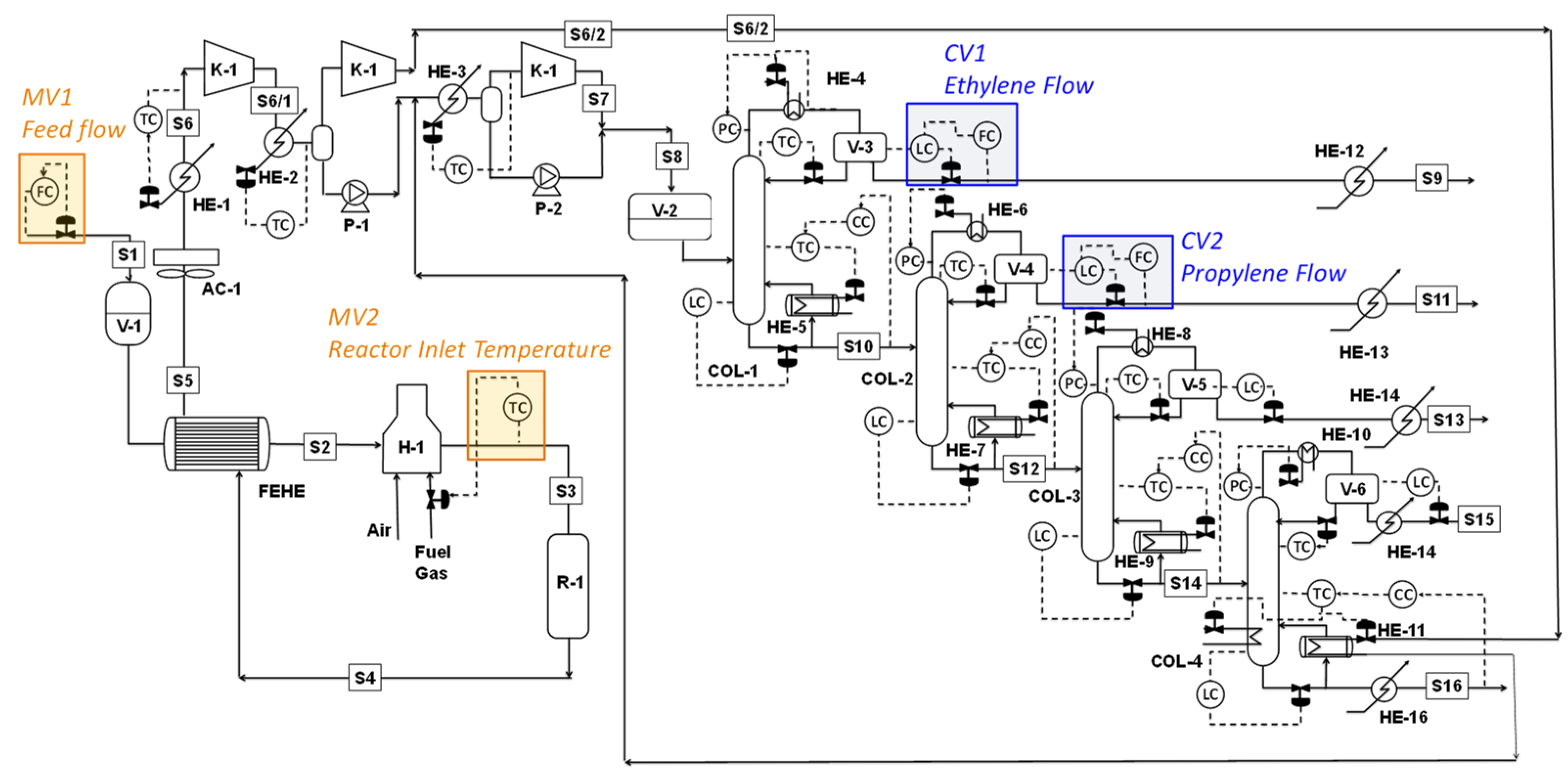
Figure 1 presents the flowsheet of the 2-butene metathesis process [25]. The fresh feed is a mixture of 2-butene (reactant) and n-butane (inert) in a 70:30 mol% ratio. The unit is designed to process 5.7 t/h of fresh feed coming from the fluid catalytic cracking unit. The plant includes a preheating/heating section where the feed is preheated by the feed-effluent exchanger (FEHE) and by the heater (H-1). The reactor inlet temperature is adjusted by the furnace duty via a temperature controller. The reaction takes place in an adiabatic tubular reactor with a tungsten oxide catalyst supported on silica. The reactor, with a diameter of D = 3 m and a length of L = 9 m, operates at P = 1.0 bar and T = 550 °C. The residence time is 34 s. The reactor effluent preheats the fresh feed in the FEHE and then is further cooled in an air cooler (AC-1) and water cooler (HE-1) prior to entering the separation section. The reactor outlet mixture temperature is controlled by the HE-1 cooler upstream of the compression section to ensure an acceptable temperature (circa 50 °C) at the inlet of the K-1 compressor. The heat generated by compression is recovered in the reboiler (HE-11) of the last distillation column. A train of four distillation columns recovers the products, in order of decreasing volatilities: ethylene, propylene, butane–butene (C4) mixture, pentene, and hexene.

Each distillation column in the separation section has pressure and level loops for inventory control. The pressure is controlled by the condenser duty, and the liquid hold-ups are maintained by the level controllers. This approach is suitable for small reflux and boil-up ratios [26]. For each distillation column, indirect composition control is used to regulate the distillate product specification. This control is achieved through a temperature controller placed on the sensitive tray, which adjusts the reflux rate [27].

To ensure high purity in the distillate flows and prevent any light product carryover in the bottom flow, a combination of cascade control using composition control (XC) and temperature control (TC) is implemented. This control strategy follows industrial practices, where the samples are periodically taken and analyzed. Thus, we consider that the composition controller experiences a 10 min sampling period and a 10 min dead time. Particularly, the HE-11 reboiler duty from the pentene distillation column receives a constant heat duty from the compression work generated to increase the pressure of the reactor effluent, with any remaining heat supplied by low-pressure steam.

The model predictive control is applied on a supervisory level, acting directly on the set points of the feedback control loops (manipulated variables) in order to achieve the product flow targets (controlled variables) set by the user. The LMPC system is composed of two manipulated variables, the setpoints of the fresh feed controller (MV1) and of the reactor inlet temperature controller (MV2), and two controlled variables, ethylene and propylene flows. Thus, there is a two-layer structure for LMPC implementation. The first layer consists of regulatory decentralized PI/P loops that stabilize the main process variables. The second (supervisory) layer is the LMPC controller, which adjusts the set points of conventional regulatory loops. Figure 1 illustrates the plantwide control of the 2-butene olefin metathesis, showcasing the input–output variables in a 2 × 2 configuration.

2.2. Controller Tuning

The algorithms used for the feedback controllers are proportional (P) and proportional-integral (PI). All column sumps level controllers are P-type controllers (large value of the reset time Ti) with a gain of 1%/%, where the process variable (PV) and controller output (OP) ranges are set to twice the nominal value.

For temperature, pressure, and the other level controllers, the reset time was set to an estimated value of the process time constant [28]. The gains (Kc) were set by trial and error.

The composition controllers, which must deal with the dead time and sampling of the composition measurement, are tuned by conducting a relay-feedback test and applying the Tyreus–Luyben tuning rule. The resulting tuning parameters and the corresponding controller action are presented in

Table 1. Regulatory controllers tuning parameters and ranges.

Controller	PV, Value and Range	OP, Value and Range	Kc (%/%)	Ti (min)	Controller Action
Heater
TC	Temperature = 550 °C	Duty = 0.42 MMkcal/h	2	4	Reverse
	540 … 560 °C	0.1 … 0.6 MMkcal/h
COL-1
PC	Pressure = 32 bar	Condenser duty = −0.07 MMkcal/h	25	5	Reverse
	30 … 35 bar	−0.14 … 0 MMkcal/h
LC	Reflux drum level = 1.967 m	Distillate rate = 270 kg/h	1	60	Direct
	1.5 … 2.4 m	0 … 750 kg/h
TC	Stage 7 temp. = −1.21 °C	Reflux rate = 1009 kg/h	15	5	Direct
	−6 … 6 °C	500 … 3000 kg/h
LC	Sump drum level = 1.037 m	Bottoms product rate = 5401 kg/h	1	60	Direct
	0 … 2.075 m	0 … 10,798 kg/h
TC	Stage 23 temperature = 113.4 °C 0 … 226.1 °C	Reboiler duty = 0.365 MMkcal/h 0 … 0.729 MMkcal/h	5	30	Reverse
CC	Online analyzer = 0.8 wt% (C2)	Temperature = 113. 4 °C	0.07	145	Direct
	0 … 0.15% wt%	0 … 226.8 °C
COL-2
PC	Pressure = 17 bar	Cond. duty = −0.41 MMkcal/h	20	12	Reverse
	15 … 19 bar	−0.53 … −0.35 MMkcal/h
LC	Reflux drum level = 2.55 m	Distillate rate = 1043 kg/h	1	10	Direct
	2.25 … 3 m	0 … 3100 kg/h
TC	Stage 3 temp. = 42.9 °C	Reflux rate = 4731 kg/h	5	10	Direct
	40 … 45 °C	2000 … 7500 kg/h
LC	Sump drum level = 0.94 m	Bottoms product rate = 4357 kg/h	1	60	Direct
	0 … 1.88 m	0 … 8705 kg/h
TC	Stage 34 temp. = 115.2 °C	Reboiler duty = 0.304 MMkcal/h	1	30	Reverse
	105 … 125 °C	0.15 … 0.6 MMkcal/h
CC	Online analyzer = 0.3 wt% (C3)	Temperature = 115.2 °C	0.065	198	Direct
	0 … 0.15% wt%	0 … 150 °C
COL-3
PC	Pressure = 3.9 bar	Cond. duty = −0.47 MMkcal/h	20	12	Reverse
	3.5 … 4.5 bar	−0.93 … 0 MMkcal/h
LC	Reflux drum level = 3.75 m	Distillate rate = 2372 kg/h	1	15	Direct
	3 … 4 m	0 … 4729 kg/h
TC	Stage 3 temp. = 42.1 °C	Reflux rate = 3180 kg/h	3	10	Direct
	37 … 47 °C	500 … 5000 kg/h
LC	Sump drum level = 0.68 m	Bottoms product rate = 1984 kg/h	1	60	Direct
	0 … 1.36 m	0 … 3975 kg/h
TC	Stage 28 temperature = 88.8 °C 75…95 °C	Reboiler duty = 0.304 MMkcal/h 0 … 0.7 MMkcal/h	1	20	Reverse
CC	Online analyzer = 0.12 wt% (2-Butene)	Temperature = 88.8 °C	0.04	105	Direct
	0.05 … 0.3% wt%	0 … 177 °C
COL-4
PC	Pressure = 1.15 bar	Condenser duty = −0.25 MMkcal/h	20	12	Reverse
	1 … 1.5 bar	−0.5 … 0 MMkcal/hr
LC	Reflux drum level = 4.175 m	Distillate rate = 1380 kg/h	1	5	Direct
	3 … 5 m	0 … 2760 kg/h
LC	Sump level = 0.575 m	Bottoms product rate = 605 kg/h	1	60	Direct
	0 … 1.15 m	0 … 1215 kg/h
TC	Stage 26 temperature = 72 °C 0 … 144 °C	Reboiler duty = 0.2 MMkcal/h 0 … 0.412 MMkcal/h	1	30	Reverse
CC	Online analyzer = 0.99 wt% (C5)	Temperature = 72 °C	0.05	170	Direct
	0.5 … 1.12% wt%	0 … 142 °C

.

2.3. Process Model Identification

In industrial applications, step tests are typically executed on the operating unit to identify a valid process model required for designing the model predictive controller. Herein, the Aspen Plus Dynamics simulation model acts as the “live” unit to extract the necessary process data for designing a 2 × 2 LMPC using MATLAB/Simulink. In this study, a doublet step signal is used for input–output data generation. The doublet test is two bump tests performed in rapid succession and in opposite directions (e.g., +/−10%). For each of the two input variables (feed flow set point and reactor inlet temperature set point), a doublet test of +/−10% amplitude is executed. In these tests, the perturbations are applied for a total duration of 30 h with data received at regular intervals of 0.1 h, which is the sampling time of the model. Thus, 300 points of data were generated to develop the models.

The test starts in a steady-state condition, which is maintained for 10 h. After 10 h, the feed flow controller set point is increased by +10% for a duration of 10 h. The control system is able to bring the plant to a new steady state. The production (ethylene and propylene flow) increases by approximately 8.1% and 5.5%, respectively. The next step test is performed at t = 20 h, corresponding to −20% from the current value, or −10% from the nominal steady. The opposite effect (production decrease) is observed. The control system brings the unit to a new steady state, where the ethylene and propylene flows decrease by approximately −5.9% and −8.4%. A final step, at t = 30 h, is performed to bring the control system to the initial conditions. The feed flow is increased by +10%. The production flow rates return to their initial values.

The same strategy is applied to the reactor inlet temperature controller set point. Starting from the nominal steady state, at t = 10 h, the temperature controller set point is increased by +5 °C for a duration of 10 h. A new steady state is reached, where the ethylene and propylene flows increase by 2.5% and 0.9%, respectively. At t = 20 h, the next step test is performed, which corresponds to a decrease of −10 °C from the current value or −5 °C from the nominal steady state. As a result of the test, the effect is opposite to the previous step, where both production flows decrease. After 10 h, the ethylene and propylene flows decrease by approximately −2.5% and −0.9%, respectively. A final step is performed at t = 30 h to bring the control system back to the initial conditions. In this final step, the reactor inlet temperature is increased by +5 °C. At t = 40 h, the production flow rates return to their initial values.

These variables are referred to as manipulated variables (MV). The outputs (controlled variables, CV) are ethylene and propylene flow rates, which are production targets set and controlled by the user through the LMPC. The list of manipulated and controlled variables for the supervisory level is shown in

Table 2. Input/output variables of the LMPC controller.

Input/Output	Nominal Value	Minimum	Maximum	Dimensionless Nominal Value	Type
Feed flow/[kmol/h]	100	75	125	50%	Manipulated variable (MV1)
Reactor inlet temperature/[°C]	550	450	650	50%	Manipulated variable (MV2)
Ethylene flow/[kmol/h]	9.6	4.8	14.4	50%	Controlled variable (CV1)
Propylene flow/[kmol/h]	24.5	16.1	33.5	50%	Controlled variable (CV2)

.

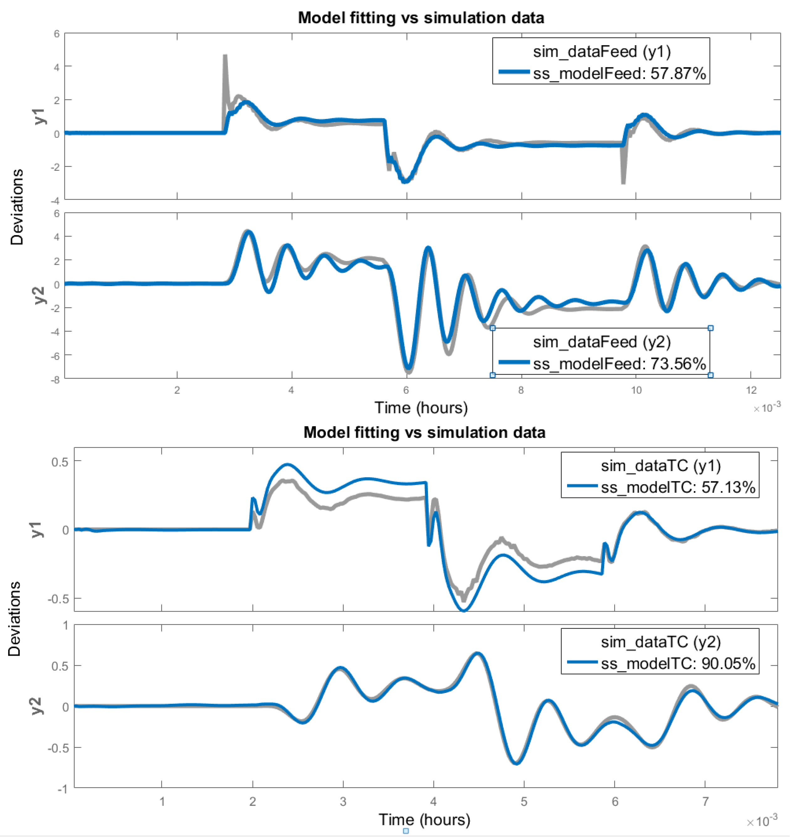
In a doublet test performed on one input, the responses of the two outputs are recorded, and a linear state space model is obtained from the input–output simulation data (ssest MATLAB function). The state–space models corresponding to the two inputs are then concatenated into a single final state–space model. The identified model has an order of 24. The system matrices A, B and C are provided in Appendix A. The models are expressed in deviations from the nominal values in order to simplify the complexity of the process model and consequently the model-based controller. The stability of the model is verified by checking the eigenvalues of the system matrix. Figure 2 displays the results from the identified model and simulation data. The results show a good agreement between the model estimates (e.g., ss_modelFeed and ss_modelTC) and the process simulation data output (e.g., sim_dataFeed and sim_dataTC). As with any model, the linear state–space representation is an approximation of the real process. However, the controller designed using this model should work despite the modeling inaccuracy.

2.4. MPC Controller Design and Tuning

LMPC is an optimization-based control approach that utilizes a linear process model to predict and optimize future process responses. At each sampling time, the model is updated based on new measurements and variables estimated using a Kalman filter considering the disturbances and measurement noise. The open-loop optimal manipulated variable moves are computed over a finite prediction horizon based on a specified cost function. These calculated manipulated variables are then implemented for the subsequent prediction horizon. The prediction horizon is typically shifted by one sampling time into the future, and the previous steps are repeated. The optimization problem for prediction is solved based on a linear time-invariant model. Nowadays, state–space models are commonly used for representing the linear time-invariant models in MPC applications.

The LMPC algorithm can be described by the following optimization problem:

$$\underset{\Delta u\left(k\right)...\Delta u(k+m-1)}{min}{\sum }_{i=1}^p\left|\right|{\Gamma }_i^y\left(\right[y(k+1)\left|k\right)-r(k+1)]{\left|\right|}^2+{\sum }_{i=1}^m\left|\right|{\Gamma }_i^u(\left[\Delta u\right(k+l-1){\left|\right|}^2$$

(1)

$$\dot{x}(k+1)=Ax\left(k\right)+Bu\left(k\right)$$

(2)

$$y\left(k\right)=Cx\left(k\right)$$

(3)

$$\Delta u=\left\{\Delta u\right|\Delta {umax}_{min}\}$$

(4)

where ${\Gamma }_i^y$ and ${\Gamma }_i^u$ are weighting factors of each component of input (u) and prediction output (y), respectively. The matrices A, B, and C are the state–space matrices of the linear model around a nominal operating point. For the given reference set point (r), the LMPC uses the model to predict the future behavior of the process output (y) and calculates the future control moves (Δu), which minimizes the control error (r − y). The number of prediction horizon (p) and control horizon (m) points, respectively, determines the prediction of y and Δu. Recommended values for the prediction and control horizon are provided in [1]. For the prediction horizon, values between 10 and 30 are suggested. Higher values result in less aggressive control actions and slower response but require more computational effort. Lower values can lead to instability and more aggressive control actions. For the control horizon, values between 1 and 4, or approximately 1/3 of the prediction horizon, are recommended. These values ensure good control performance with reduced computational effort and improved robustness.

In this work, the prediction horizon is set to p = 10, while the control horizon is set to m = 2. The output weight is set to the nominal value for each variable, indicating equal importance for all output variables. Note that, although the control action Δu is calculated for m future steps, only one control action is actually implemented, the optimization being repeated at each sampling time.

In this study, the MPC controller ensures that the production flows of ethylene and propylene meet the user-defined targets. This is achieved by adjusting the set points of the conventional control loops, the feed flow set point (MV1), and the reactor inlet temperature set point (MV2). This strategy enables the control problem to be addressed globally, taking into account the interactions between the variables to optimize the overall system performance [1]. An alternative approach to address the control problem in the system could be subsystem partitioning. This involves dividing the unit into distinct sections, such as the reaction section and the separation section. Each section would then be treated as a separate entity, and a dedicated model predictive controller (MPC) can be designed for each section [10].

2.5. Model Predictive Control Implementation

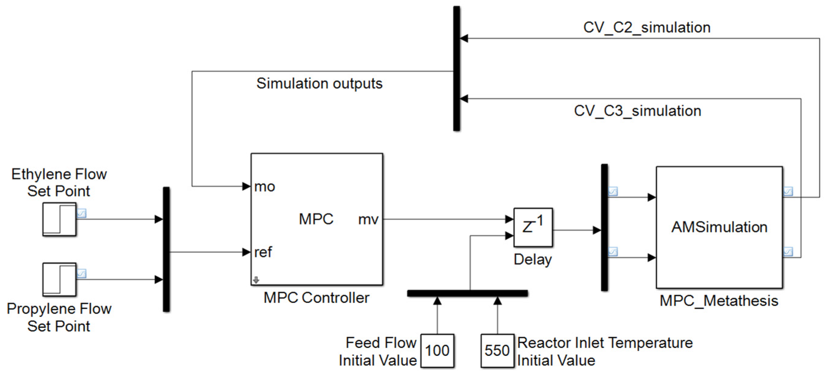
MATLAB environment is used to enable the connection between the dynamic simulation in Aspen Plus Dynamics and the model-based controller configured in MATLAB/Simulink. To establish the connection between the two software platforms, MATLAB/Simulink employs an ActiveX automation server to interact with process simulators. The Simulink environment provides a convenient interface for integrating the controller and the dynamic simulation. It allows for the exchange of data and control signals between MATLAB/Simulink and Aspen Dynamics. Note that proper selection of the MATLAB version and Aspen Plus Dynamics software is essential to ensure communication without compatibility issues between the two platforms. In this study, MATLAB version R2015b (32 bits) and Aspen Plus Dynamics version 10 (also 32 bits) are selected. The Mathworks Matlab MPC toolbox ^® was successfully used in this work. The LMPC is then implemented in Simulink, which drives the Aspen Plus Dynamics model (Figure 3).

3. Results and Discussion

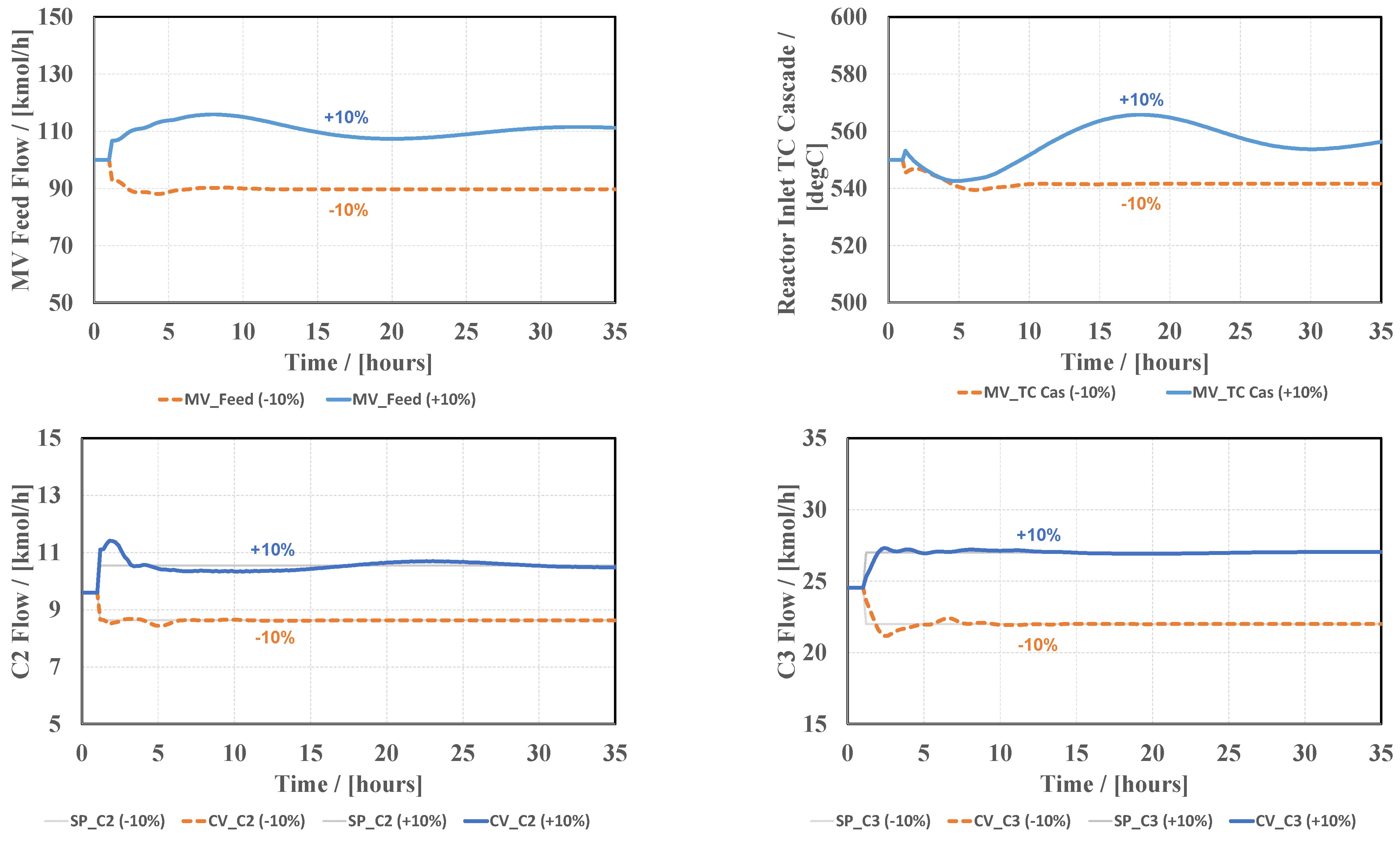
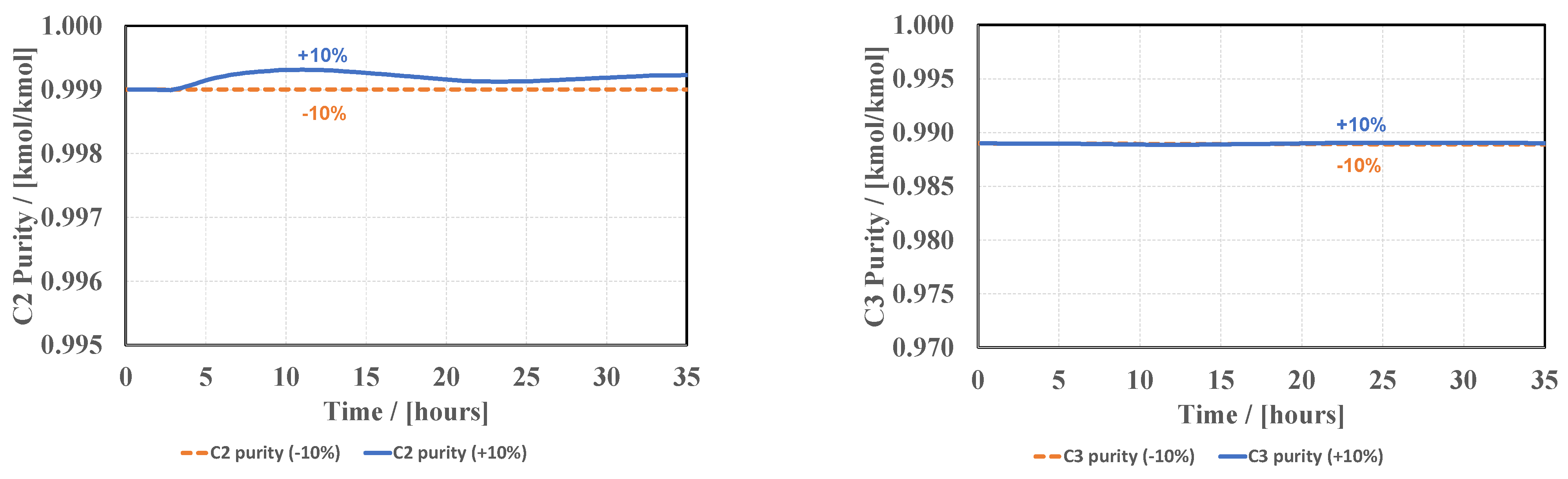
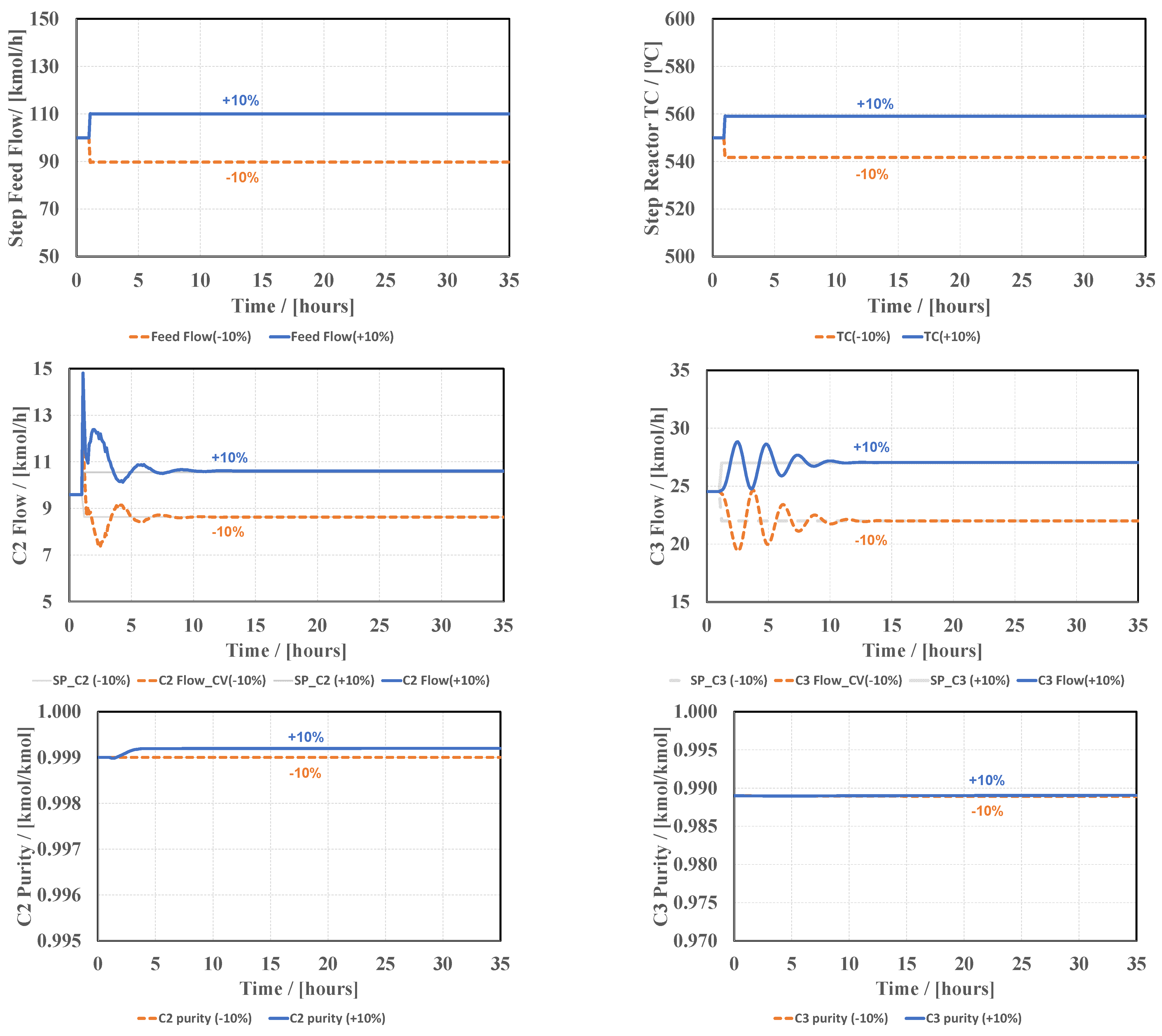
The control performance of the LMPC controller is evaluated through tests of step changes applied on the setpoints of the controlled variables. The tests are conducted after 1 h of steady-state operation. Two sets of data are generated, for a step change of +10% (continuous solid blue line) simultaneously applied to both controlled variables (e.g., ethylene and propylene flow) and −10% (dashed orange line) applied to the same controlled variables. These tests give the dynamics of the controlled and manipulated variables under closed-loop conditions. Note that the values of the manipulated variables at the new steady state could be implemented as steps in order to achieve the same final change of the controlled variables, but in an open-loop fashion.

The LMPC controller demonstrates stable and rapid attainment of the target production rates within a reasonable duration of less than 5 h (Figure 4). The overshoot of the flow set points is minimal. The constraints on the manipulated variables were not active. Some oscillations in the feed rate and reactor inlet temperature are observed. Specifically, for a +10% step change in production flows, the model drives the reactor inlet temperature set point in the opposite direction. However, after a few hours, the LMPC corrects this manipulated variable and aligns it in the correct direction, resulting in the attainment of the desired targets for both controlled variables. Accurate control of product purities is achieved, for both ethylene (C2) and propylene (C3) products. Overall, the LMPC effectively manages to reach the target production rates, with minimal overshoot and proper adjustment of manipulated variables over time.

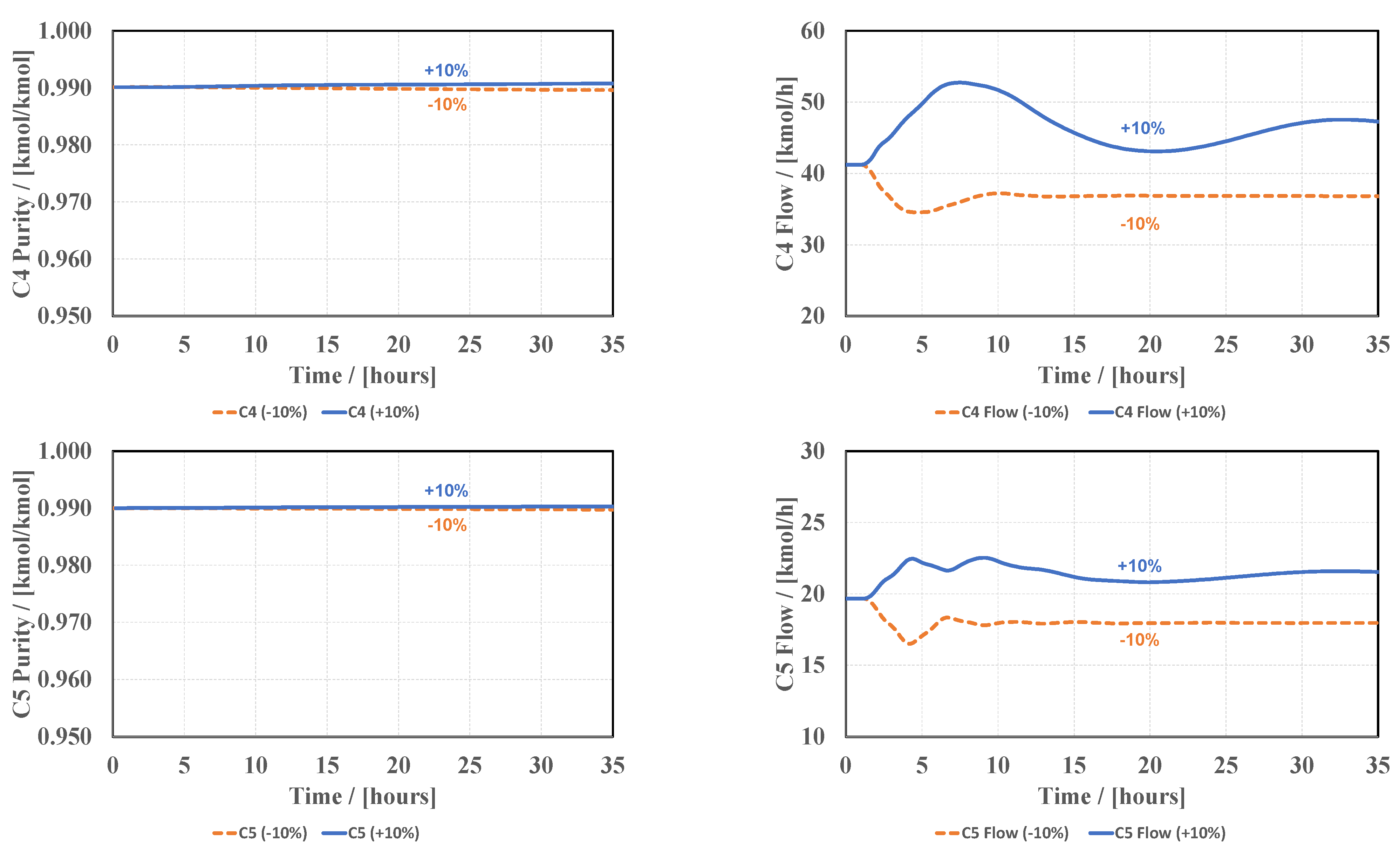
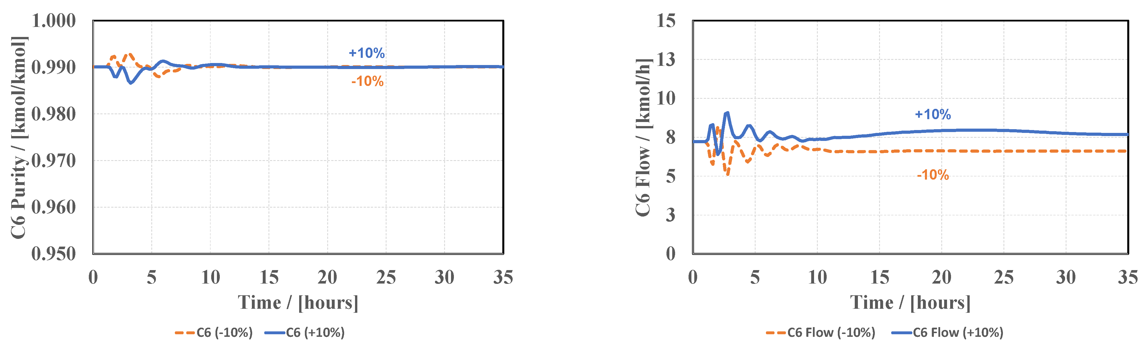
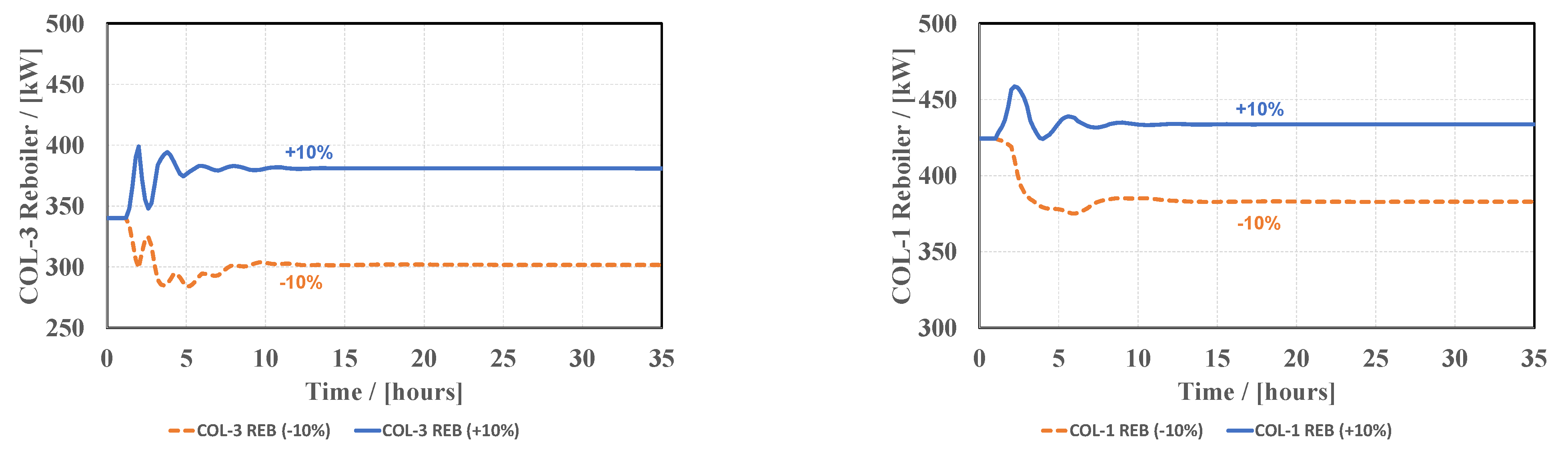
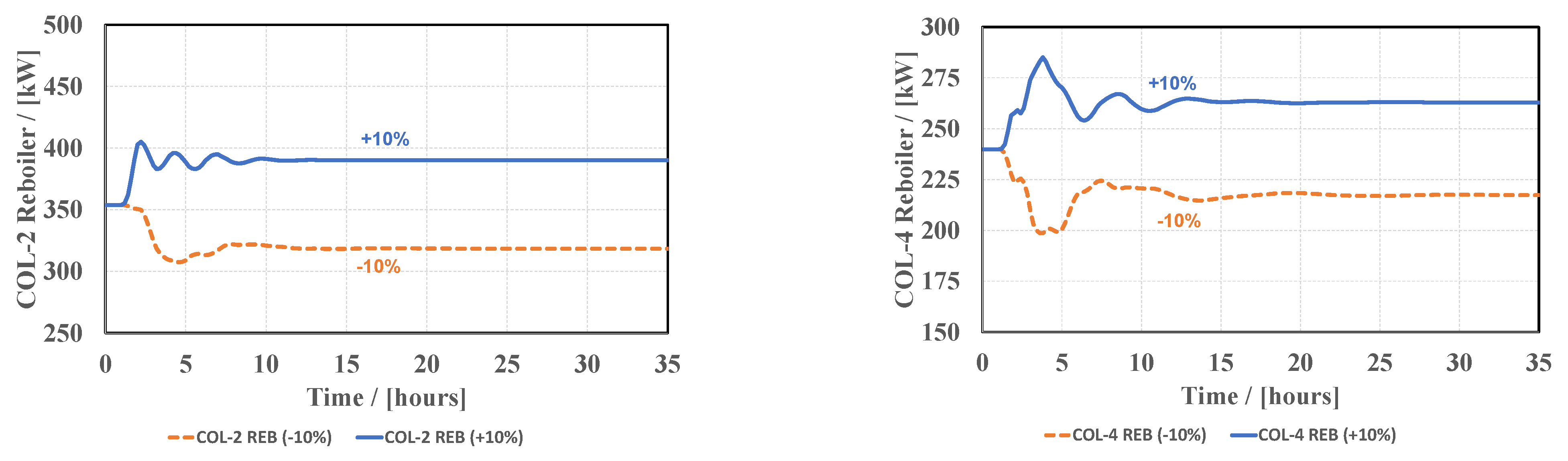
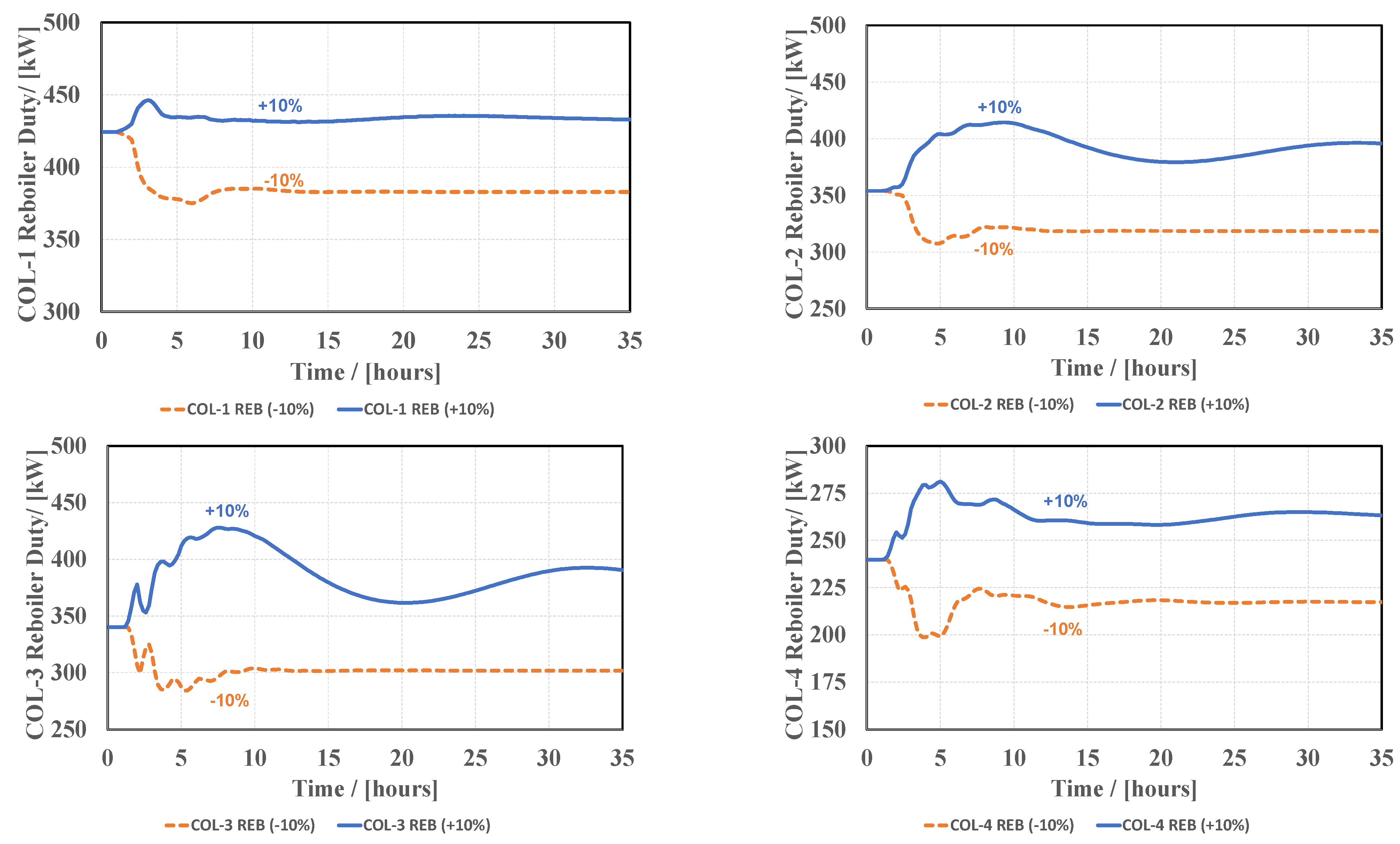
Figure 5 depicts the remaining product flows (butane and butene (C4), pentene (C5), and hexane (C6)) together with their corresponding purities. Figure 6 shows the columns’ reboiler duties. The model predictive controller indirectly affects these variables as any changes made to the manipulated variables have a corresponding influence on these outputs. However, the feedback control mechanism effectively adjusts these variables within acceptable limits.

Notably, the response to the −10% step change (represented by the orange dashed line) is faster compared to the +10% step change. This indicates that it is easier to decrease the production rate.

The performance of the LMPC is compared with the open-loop response using the dynamic simulation data. In the open-loop test, the manipulated variables (feed flow set point and reactor inlet temperature set point) are modified by applying a step such that the output variables (C2 flow and C3 flow) change by +/−10% from their steady-state values (as in the LMPC tests). In this way, the two control strategies could be compared by means of performance indexes such as integral square error (ISE), mean square error (MSE), integral absolute error (IAE), peak error (PE), or overshoot. Results are presented in Figure 7 and Figure 8.

In Figure 7 and Figure 8, the open-loop responses demonstrate reasonable control with some oscillations until reaching the production flow targets after approximately 15 h, followed by a steady-state regime. The ethylene flow exhibits an overshoot of approximately 50% compared to the set point value; however, the feedback controllers efficiently adjust and swiftly reduce the error. Throughout these tests, the feedback controllers effectively maintain the product purities of ethylene and propylene at their respective set points for both control strategies. Albeit the nonlinearity of the 2-butene olefin metathesis unit, the results show that the linear model predictive controller outperforms the open-loop response.

To characterize system performance and identify the most effective control structure, several performance indexes are considered. The mean square error loss (MSE) is utilized to illustrate the performance and control response for the same step change of +/−10% in production flow over a period of 30 h. The MSE represents the sum of squared differences between predicted and actual output values, divided by the number of tested hours.

Additionally, the integral square error (ISE) is employed as another measure to evaluate system performance, calculated by integrating the square of the control error over the same period (by applying the trapezoidal rule, with a fixed 0.2 h step). In industrial practice, the control performance is often assessed based on the maximum deviation of the controlled variables, referred to as peak error (PE). However, while PE identifies the maximum deviation, it does not provide information about fluctuations or the ability to achieve the set point. Therefore, the integral absolute error (IAE) is commonly used to evaluate control response and accuracy. The IAE calculates the sum of areas above and below the set point, equally penalizing errors regardless of direction.

The results presented in

Table 3. Index performances of control strategies.

		Controlled Variable 1: Ethylene Flow (y1)				Controlled Variable 2: Propylene Flow (y2)
Method	U.M	MPC	Open Loop	MPC	Open Loop	MPC	Open Loop	MPC	Open Loop
		−10%	−10%	+10%	+10%	−10%	−10%	+10%	+10%
ISE	(kmol/h)2 × h	0.05	3.16	1.34	6.19	1.7	15.8	1.3	10.6
MSE	(kmol/h)2/h	0.01	1.05	0.22	2.06	0.3	5.3	0.2	3.5
IAE	(kmol/h) × h	0.50	5.63	4.80	9.35	2.8	20.8	3.3	16.2
PE	kmol/h	0.20	3.57	0.86	4.26	1.6	2.7	1.7	2.4

consistently indicate that the LMPC exhibits significantly better performance compared to open-loop responses, demonstrating its superior control capabilities.

Challenges, Recommendations, and Opportunities

The performance of the model predictive controller (MPC) is highly dependent on the quality of the process model. The implementation of an LMPC typically involves obtaining a linear model through system identification directly applied to the industrial plant. This is the most common method. However, when dynamic simulation of the process is available, system identification offers a significant advantage by obtaining models based on input–output simulation data. In this context, it is essential that the dynamic simulation accurately reproduces the dynamics of the industrial process. The MPC can be set up offline and applied to either a virtual (for initial testing) or an industrial unit (some adjustments might be required). This approach stands out for its simplicity and practicality in diverse industrial applications.

Alternatively, the linear model can be obtained by linearization of the dynamic simulation model. This approach works well when a simple process (such as stirred reactor, vapor–liquid separator, or binary distillation with ideal mixtures) is considered. If the dynamic simulation model is a faithful representation of the real plant, the LMPC controller designed in this way outperforms an LMPC designed based on an identified process model.

However, when dealing with complex and nonlinear processes, linearization of the dynamic simulation model might not work. In our experience, the linear model is often unstable and, despite time-consuming efforts for model reduction and scaling, useless for the design of the LMPC. This is the rationale behind the predominant utilization of LMPC on individual equipment or sections of the plant, and not plant wide. From the authors’ experience, working with variables expressed as scaled deviations from the steady-state values (instead of absolute values) significantly improves the performance of the designed controller. Irrespective of the method employed, significant time and expertise are devoted to model development and validation. Finally, a post-implementation review of the industrial unit and continuous follow-up of the linear models during unit operation by experienced specialists are compulsory. Changes in process, such as catalyst change-out, unit revamps or modernization, heat integration, etc., require re-validation of the process model.

From the industrial experience of one of the authors, the MPC is widely accepted as a necessary profitability solution for many applications. However, the current market dynamics impede sustainable MPC performance. Thus, the resources of experts, needed to monitor and maintain MPC, are becoming limited. The commissioning of MPC might not be an issue where, typically, an expert user employs the model identification. However, the responsibility for maintenance and monitoring of MPC is often placed on individuals who may not have expertise in the field. This includes re-identifying models. For this reason, a common practice is to employ a first-order plus dead time model (FOPDT), which does not ensure an optimal process model. Another approach is adaptive MPC by automated closed-loop testing. Multiple industrial applications have successfully been applied [29]. Future work should include efforts to enhance operator interaction with MPC through user-friendly interfaces, while also implementing effective performance monitoring and maintenance strategies despite limited resources.

4. Conclusions

This study demonstrates that the 2-butene olefin metathesis process can be controlled by a linear 2 × 2 model predictive controller. The dynamic simulation of the process, specifically the reaction–separation flowsheet, served as the basis for the “operating” unit. The flow rates of ethylene and propylene, the main products of the process, were the controlled variables. The set points of the fresh feed flow and the reactor inlet temperature controllers were the manipulated variables. Doublet tests were performed on the Aspen Plus Dynamics simulation of the plant to collect process data for model identification. A linear state–space model was obtained using MATLAB’s state–space estimation. The accuracy of the identified model was validated by comparing it against the dynamic simulation. MATLAB was utilized for the configuration and tuning of the LMPC following recommended guidelines for setting the prediction and control horizons.

To assess the performance of the LMPC, two sets of tests were conducted, involving simultaneous changes in production flows (+/−10%). The LMPC effectively manipulates the feed and reactor inlet temperature set points to achieve the new production rates. The performance of the MPC was compared with the open-loop response from the dynamic simulation using various performance indexes such as ISE, MSE, IAE, PE, and overshoot.

The results demonstrated that the LMPC outperformed the open-loop response in both tests, showcasing better performance for +/−10% production flow rate changes. The LMPC consistently exhibited much lower errors (by a factor of 10) compared to the open-loop response. This outcome reveals the benefit of model-based control attaining new production rates much faster than conventional process control.

While alternative methods such as Aspen Dynamics linearization and model reduction exist for developing linear process models, the applicability of this technique in industrial applications is very limited due to nonlinear behavior, large size, and potential instability of the Aspen Dynamics models.

In summary, this study demonstrates the applicability of a linear MPC controller on the 2-butene olefin metathesis process. The MPC is configured on a supervisory level, providing set points to conventional controllers. The findings contribute to the understanding of advanced control strategies for complex processes and emphasize the importance of model quality, selection, and proper tuning in achieving superior control performance.