Equipment Disassembly and Maintenance in an Uncertain Environment Based on a Peafowl Optimization Algorithm

Abstract

Disassembly sequence planning (DSP) is a key approach for optimizing various industrial equipment-maintenance processes. Finding fast and effective DSP solutions plays an important role in improving maintenance efficiency and quality. However, when disassembling industrial equipment, there are many uncertainties that can have a detrimental impact on the disassembly and subsequent maintenance work. Therefore, this paper proposes a multi-objective DSP problem in an uncertain environment that addresses the uncertainties in the disassembly process through stochastic planning, with the objectives of minimizing disassembly time and enhancing responsiveness to priority maintenance components. Due to the complexity of the problem, an improved peafowl optimization algorithm (IPOA) is proposed for efficient problem-solving. The algorithm is specifically designed and incorporates four customized optimization mechanisms: peafowls’ courtship behavior, the adaptive behavior of female peafowls in proximity, the adaptive search behavior of peafowl chicks, and interactive behavior among male peafowls. These mechanisms enable effective search for optimal or near-optimal solutions. Through comparisons with a real-world industrial case and other advanced algorithms, the superiority of the IPOA in solving DSP problems is demonstrated. This research contributes to improving maintenance efficiency and quality, bringing positive impacts to industrial equipment maintenance.

1. Introduction

In today’s industrial domain, the paramount importance of ensuring the safety, stability, and efficient operation of equipment cannot be overstated [1]. To attain this objective, equipment maintenance, by replacing or repairing defective, damaged, or worn-out components to ensure uninterrupted equipment functionality, assumes a pivotal role [2]. In the context of equipment maintenance, the meticulous arrangement of the disassembly sequence holds critical significance. Disassembly sequence planning (DSP) denotes the systematic disassembly operations executed in accordance with predetermined steps and procedures [3]. A well-structured disassembly sequence yields numerous advantages. Firstly, it ensures the timely completion of maintenance tasks. Time constraints often accompany equipment maintenance due to the adverse repercussions of protracted downtime, namely reduced production efficiency and financial losses [3]. Employing an optimal disassembly sequence enables the efficient and methodical dismantling of parts, thereby enhancing the speed and efficacy of maintenance activities and facilitating the punctual accomplishment of tasks. Secondly, the acquisition of an optimal or near-optimal disassembly sequence is highly advantageous for the judicious allocation of manpower and resources [4]. If the disassembly sequence is rationally arranged, human resources can be allocated effectively, mitigating redundancy or repetition and maximizing workforce efficiency. Furthermore, a well-considered disassembly sequence optimizes the utilization of material resources, curtails component losses and waste, and ultimately reduces maintenance costs [5].

Indeed, the disassembly process in equipment maintenance is subject to uncertainties arising from various factors such as the maintenance history, usage conditions, and extent of equipment damage [6]. These uncertainties can significantly impact the complexity and difficulty of the disassembly process, thereby rendering the determination of an optimal disassembly sequence more challenging [7]. Consequently, the study of DSP within the context of uncertain environments pertaining to industrial equipment maintenance holds immense practical value.

Conducting relevant research in this domain enables the exploration and development of algorithms and methodologies for identifying the optimal disassembly sequence for different equipment types [8,9,10]. Such endeavors provide practical tools and guidance for the industrial sector, empowering companies to optimize their equipment-maintenance processes [11]. By enhancing maintenance efficiency and quality while concurrently reducing costs and risks, these research outcomes offer tangible benefits [12].

The primary motivation behind this research lies in addressing the aforementioned challenges and uncertainties associated with equipment disassembly [13]. By striving to advance the field of DSP in the face of uncertain environments, the research endeavors to contribute valuable insights and practical solutions that can be directly applied in industrial settings [14]. Ultimately, the objective is to assist organizations in achieving optimal equipment maintenance outcomes, bolstering operational efficiency, and minimizing associated risks and expenses.

To address the aforementioned objectives, a multi-objective mathematical model was developed for disassembling industrial equipment in an uncertain environment with the aim of minimizing disassembly time while improving responsiveness to priority maintenance components. Recognizing the NP-hard nature of the DSP problem, an IPOA was specifically designed to tackle it. The IPOA involved redefining the optimization operators of the POA and utilizing a stochastic simulation method to address the inherent uncertainties within the model. This novel approach offers fresh insights into enhancing the efficiency of industrial equipment maintenance through DSP.

The remaining sections of this paper are structured as follows: Section 2 provides a comprehensive review of DSP problems, offering a thorough understanding of the existing literature and research in this area. Section 3 outlines the modeling approach adopted in this study, presenting the construction of the proposed mathematical model. Section 4 introduces IPOA, the customized algorithm developed to solve the DSP problem. Section 5 validates the effectiveness of the proposed method and algorithm through a real-world industrial case study, illustrating the superior performance of IPOA in comparison to other advanced algorithms. Finally, the paper concludes by discussing the findings and limitations and suggesting potential avenues for future research in this domain.

2. Literature Review

Since its inception, DSP has garnered considerable attention among scholars. They have developed various graph theory models associated with DSP, including AND–OR graphs, disassembly mixed graphs, and disassembly trees [15]. These models have been tackled using both exact solvers and heuristic algorithms for problem resolution [16].

However, DSP has been proven to be an NP-hard problem, signifying that its computation time grows exponentially with task size. Exact solvers and heuristic algorithms struggle to meet the solution requirements [17]. Consequently, researchers have gradually shifted from using exact solvers to employing metaheuristic algorithms for solving DSP problems. For instance, Yu et al. enhanced the whale optimization algorithm and applied it to their energy-constrained DSP problem [18]. Zhang et al. proposed an improved social engineering optimizer for solving their constructed DSP model [19]. Wu et al. introduced a simplified gravitational search algorithm to optimize DSP for hydroelectric-equipment maintenance [20]. Zhan et al. conducted research on DSP for recycling used energy vehicle batteries, aiming to minimize energy consumption and the hazard index. They designed an improved northern goshawk optimization algorithm (NGO) for this purpose [21]. Mahmoudi et al. studied a selective DSP problem within the context of building selections, focusing on decomposition sequence time, cost, and environmental impact. They designed a non-dominated sorting genetic algorithm (NSGA-II) to optimize these objectives [22]. Sun et al. developed an improved multi-objective evolutionary algorithm based on a multiple-neighborhood search strategy to solve their proposed multi-objective asynchronous parallel selective DSP [23]. The objective was to minimize disassembly time while maximizing disassembly profit. Chen et al. proposed an optimization algorithm based on Q-learning to optimize the DSP problem of discarded smartphones [24]. Ji et al. improved the immune algorithm to find the optimal or near-optimal disassembly sequence [25]. Kheder et al. customized and enhanced the genetic algorithm, considering variations in component volume, tool change, and disassembly direction in their research [26].

It is important to note that there are inherent uncertainties in the DSP process that have been considered and analyzed by researchers. For example, Fu et al. addressed this issue by using a hybrid algorithm that combines chance-constrained programming and a multi-objective multiverse optimization algorithm [27]. Their objective was to simultaneously maximize energy consumption and minimize disassembly profit while accounting for the uncertainty of operational failures in the dismantling process. Liang et al. presented a stochastic DSP problem, taking into account noise pollution and energy consumption, and they also utilized the chance-constrained approach to solve the model [28]. Tian et al. proposed a stochastic DSP problem by considering uncertain component quality and different disassembly operation costs, which they solved using a modified artificial bee colony algorithm [29]. Kim et al. focused on the DSP problem with stochastic operation time and proposed a solution algorithm based on the sample mean approximation, aiming to minimize the cost [30]. Additionally, they investigated and analyzed the stochastic multiproduct DSP problem in another study [31]. Yeh et al. used a simplified swarm algorithm to handle a DSP problem with randomized operation times [32].

Furthermore, disassembly problems originate from assembly problems. Therefore, considering uncertainty in assembly problems can provide insights into DSP problems. Erel et al. proposed a beam-search-based method for the U-line stochastic assembly line balancing problem, which minimizes the total expected cost consisting of total labor cost and total expected unfinished cost [33]. Mosadegh et al. developed a hyper-heuristic simulated annealing algorithm to solve for processing time as a random variable in a multi-station assembly line, with the objective of minimizing the weighted sum of the expected total workload and idleness [34]. Sakiani et al. studied a two-stage assembly system with randomized delivery times and devised an extended genetic algorithm to solve it [35]. Moreover, Fu et al. performed a stochastic disassembly–processing–reassembly analysis of used products using a fruit fly optimization algorithm [36].

Based on the aforementioned literature review, it is evident that significant progress has been made in DSP research. However, there are still some limitations.

Firstly, there is a lack of research on DSP issues related to equipment maintenance in uncertain environments, which is a key factor in practice. In addition, the expected value model obtained in uncertain DSP problems has rarely been applied, and it has the advantages of greater flexibility and the ability to effectively subtract the complexity of the model. Lastly, the successful development of several optimization algorithms such as the peafowl optimization algorithm, which has exhibited high performance and demonstrated excellence in other problem domains, has not yet been applied to DSP problems. According to the “No Free Lunch” theorem [37] in optimization theory, no single optimization algorithm can universally and optimally solve all problems. On average, the performance of all algorithms is the same across all possible problems. In other words, any algorithm’s advantage on certain problems must be balanced by its disadvantage on others, leading to the absence of a universally superior algorithm. This theorem encourages researchers to explore and utilize specific optimization algorithms tailored for particular problems or problem classes, aiming to achieve more effective solutions. Hence, it is necessary to explore the application of the POA in DSP problems.

Based on the analysis above, this study makes the following contributions:

(1)

The present study undertakes an investigation into the DSP problem within the context of uncertain conditions. A DSP problem model is formulated based on the characteristics of equipment maintenance, with the objective of minimizing disassembly time and enhancing the response speed of priority maintenance parts.

(2)

To address the aforementioned objectives, an efficient metaheuristic algorithm named IPOA is proposed. Specifically tailored search operators suitable for DSP problems are designed within the framework of IPOA, and its superiority is empirically substantiated through comprehensive comparisons with other existing algorithms.

(3)

The efficacy of the constructed DSP problem model and the designed IPOA algorithm is substantiated through an empirical analysis of a real-world industrial case. The analysis demonstrates the superior performance and practical applicability of the model and algorithm in addressing DSP challenges encountered in industrial settings.

3. Proposed Problem

Here, we first describe the modeling approach we used (Section 3.1), after which we construct our multi-objective mathematical model (Section 3.2).

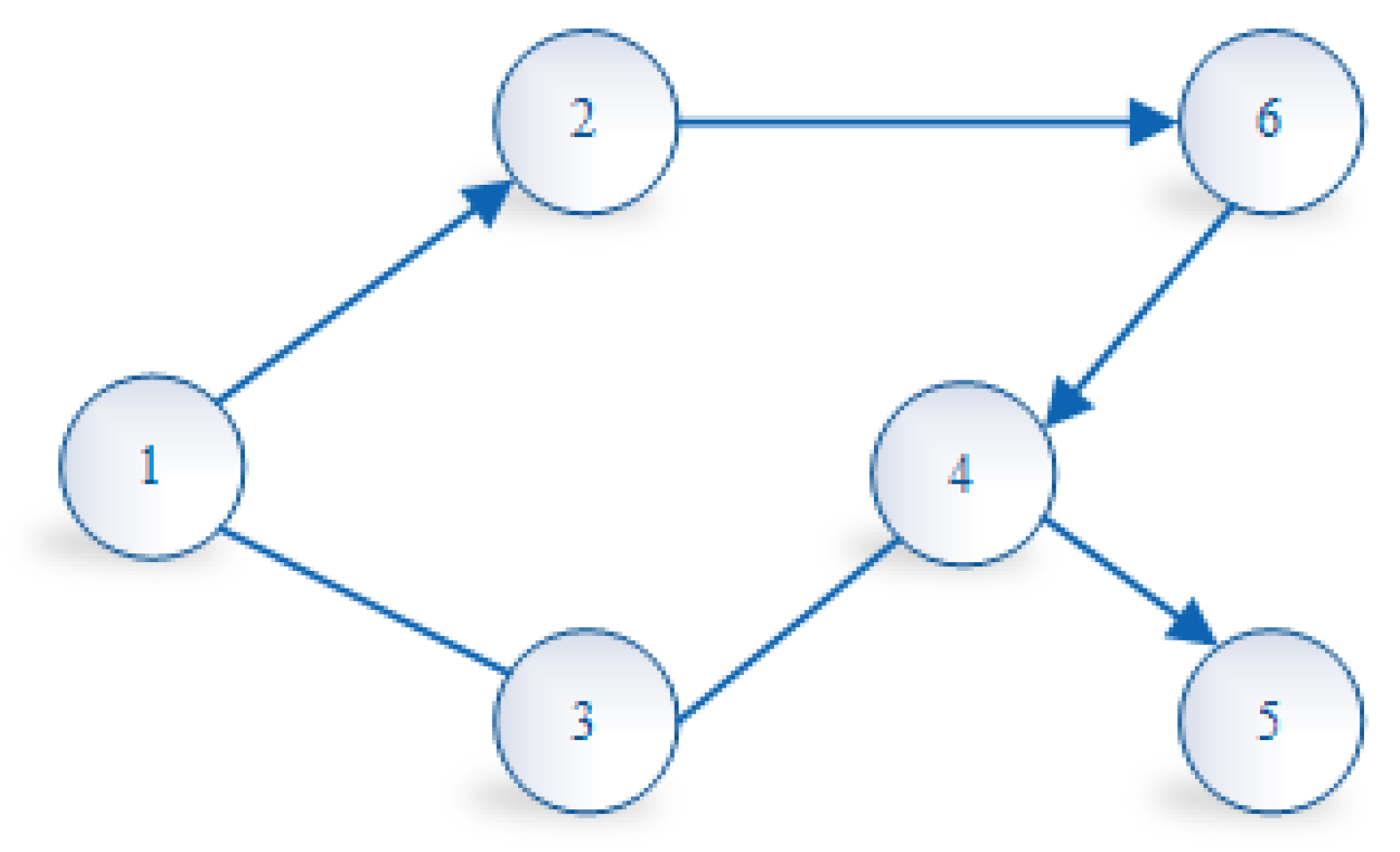
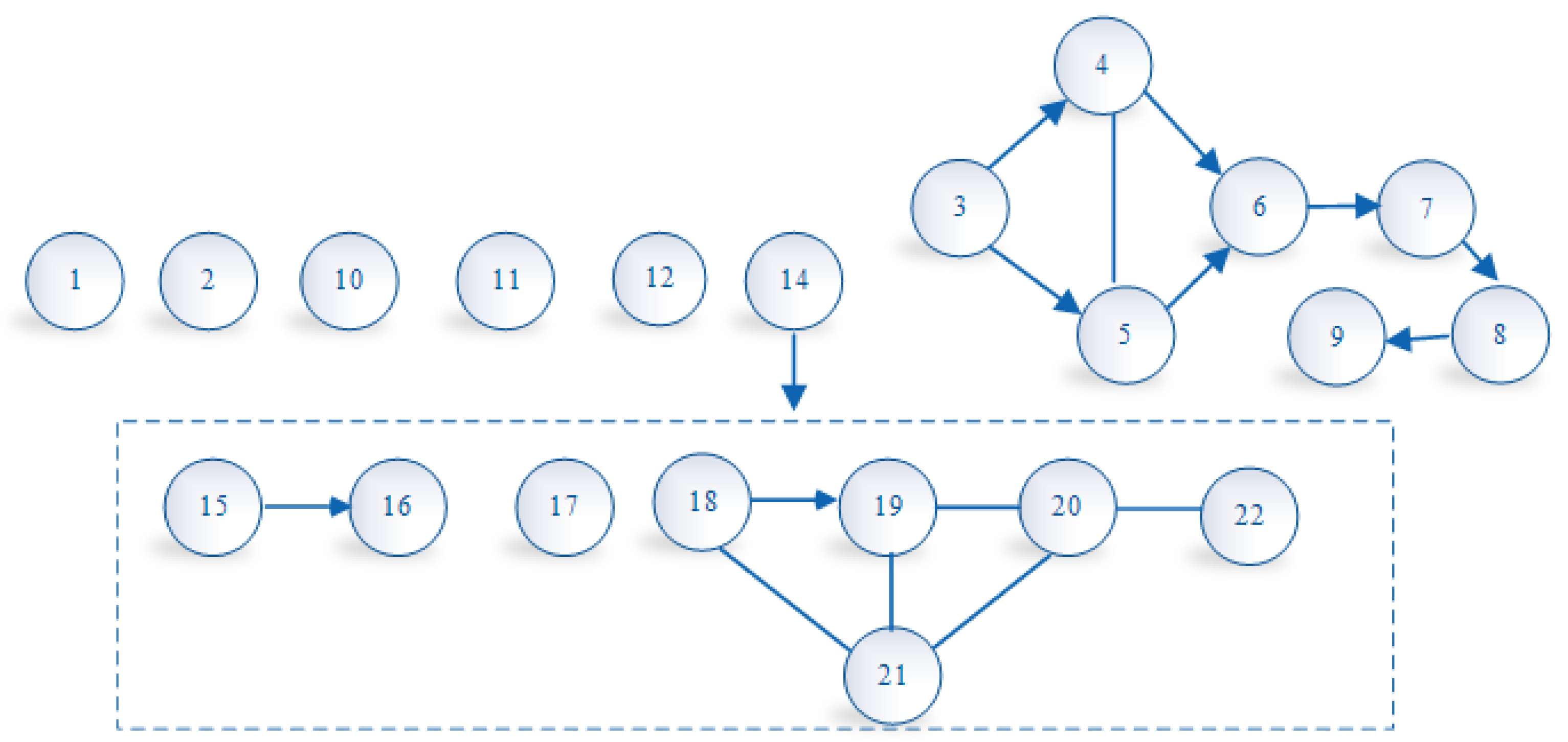
3.1. Disassembly Mixed Graph

Before proceeding with the construction of our multi-objective mathematical model, it is imperative to select an appropriate modeling approach. Among various methods available, the disassembly mixed graph stands out due to its concise, intuitive, and effective nature [21]. Its widespread application in the field further supports its suitability [21]. Hence, this paper adopts the disassembly mixed graph as the chosen modeling method. Figure 1 illustrates an example of a fundamental disassembly mixed graph for reference.

In the disassembly mixed graph, two types of relationships are present: a priority constraint relationship and a direct contact relationship. The priority constraint relationship is represented by a directed edge, indicating that one component must be disassembled before another. On the other hand, the direct contact relationship is represented by an undirected edge, denoting that the components that are in direct contact with each other.

To facilitate the representation, we can use matrices P and C to capture these relationships. In matrix P, each element P_ij is assigned a value of 1 if component i has a priority constraint relationship with component j. For example, if component 1 must be disassembled before component 2, then P₁₂ = 1. In matrix C, each element C_ij is set to 1 if component i has a direct contact relationship with component j. For instance, if components 1 and 3 have a direct contact relationship, then C₁₃ = 1.

By employing this modeling transformation, the relationships between components can be clearly demonstrated, providing a solid foundation for our subsequent research endeavors.

3.2. Proposed Model

In our constructed multi-objective model, we focus on minimizing the disassembly time and enhancing the response speed of priority maintenance components as two vital optimization objectives. This approach aims to effectively address the dual challenges faced by the maintenance team and achieve a balanced outcome.

The primary objective is to minimize the disassembly time. By reducing the time required for disassembly, we can expedite the commencement of the maintenance process and promptly restore the normal operation of the equipment. This, in turn, helps to minimize downtime, improve production efficiency and yield, and reduce production losses resulting from equipment failures. Additionally, shorter disassembly time can also minimize additional losses incurred by components and equipment during the maintenance process, leading to cost savings.

The secondary objective is to enhance the response speed of priority maintenance components. This objective entails that the maintenance team swiftly addresses the maintenance requirements of critical components of the equipment, thus effectively improving the quality of maintenance performed.

By concurrently optimizing the disassembly time and the response speed of priority maintenance components, our proposed model aims to strike a balance between these two objectives, enabling the maintenance team to achieve optimal outcomes in their operations.

The notations for the proposed optimization model are as follows:

Indices:
m:	Index of disassembly component number, m = 1, 2, …, M
Parameters:
M:	Total number of disassembly components
tm	Stochastic disassembly time required for component m (obeying uniform distribution)
gm	Difficulty of removing component m
tt	Stochastic time required to change tool (obeying uniform distribution)
td	Stochastic time required to change direction (obeying uniform distribution)
Im	Position of component m in the disassembly sequence
yn	Number of direction changes in the disassembly sequence
zn	Number of tool changes in the disassembly sequence
Decision variables:
hm	If component m has priority, hm = 1; otherwise, hm = 0.

$$Min F=\left[f1,f2\right]$$

(1)

$$f1,=E\left({\displaystyle \sum }_{m=1}^M\left(1+g_m\right)t_m+t_t{z}_n+t_d{y}_n\right)$$

(2)

$$f2={\displaystyle \sum }_{m=1}^M{I}_m{h}_m$$

(3)

$${\displaystyle \sum }_{j=1}^M{c}_{jm}\le 1$$

(4)

$${\displaystyle \sum }_{j=1}^M{p}_{jm}=0$$

(5)

$$h_m=\left\{0,1\right\}$$

(6)

Equation (1) represents the objective function to be optimized in our model, which encompasses both the minimization of disassembly time and the enhancement of response speed for priority maintenance components. Components requiring priority maintenance should be disassembled as early as possible; thus, they are represented as a minimization objective in the model. Equation (2) represents the minimization of disassembly time. The difficulty coefficients of disassembly for different components are considered, taking into account factors such as the number of direction switches and tool switches during the disassembly process. Additionally, the variable E is introduced to represent the expected objective-function value. Equation (3) represents the enhancement of response speed for priority maintenance components, with an emphasis on the early disassembly of these components. The objective is to ensure that priority components are disassembled at the earliest opportunity. Equations (4) and (5) are prerequisites for component m to be disassembled; i.e., the component must have at most one direct contact task (Equation (4)) and no prioritized tasks (Equation (5)). Equation (6) introduces a binary variable in our model, which serves as a decision variable for component disassembly.

These equations collectively form the mathematical foundation of our model, enabling us to effectively optimize the disassembly time and enhance the response speed of priority maintenance components.

4. Proposed Solution Method

POA, proposed by Wang et al. in 2021 [38], simulates the courtship, foraging, and chasing behaviors of peafowls. Interested readers can refer to the relevant literature for a comprehensive understanding of the basic concept of POA [38]. POA has demonstrated excellent performance in multiple test functions and engineering problems [38], highlighting its potential for solving DSP problems. According to the No Free Lunch Theorem [37], the continuous exploration, improvement, and application of new algorithms are necessary [29]. However, until this study, POA has not been applied in the field of DSP. Therefore, in this section, we introduce the novel multi-objective handling method and the method of peafowls’ role assignment that we utilize (Section 4.1). We further customize the courtship behavior of peafowls (Section 4.2), the adaptive behavior of female peafowls in proximity (Section 4.3), the adaptive search behavior of peafowl chicks (Section 4.4), the interactive behavior among male peafowls (Section 4.5), and the handling of uncertainty in our proposed model (Section 4.6). Finally, we provide an overall algorithm framework for the IPOA (Section 4.7).

4.1. Multi-objective Handling

When dealing with multi-objective optimization problems, there are multiple decision variables and multiple objective functions that need to be optimized. Two commonly used methods for assessing solution quality and selecting appropriate solutions are Pareto dominance and crowding distance calculation.

(1)

Pareto dominance [21,39]:

• For two given solutions, solution A and solution B, solution A dominates solution B if it is at least as good as solution B in all objective functions and better than solution B in at least one objective function.
• Dominating solution B indicates that solution A achieves better performance in multiple objective functions, regardless of whether the objective functions are to be maximized or minimized.
• The Pareto optimal solution set consists of solutions that are not dominated by any other solution in the entire solution space.

By utilizing Pareto dominance, we can identify a set of non-dominated solutions, providing a range of feasible optimization choices with trade-off relationships among the objective functions.

(2)

Crowding distance calculation [21,39]:

• Crowding distance calculation evaluates the density of solutions to select appropriate solutions in the Pareto optimal solution set.
• By assessing the distribution of solutions in the objective space, crowding distance calculation measures the density of solutions around a particular solution.
• A higher crowding distance of a solution indicates that it is more scattered in the objective space, thereby implying better diversity.

Selecting solutions with higher crowding distance helps maintain diversity in the population, prevents solutions from being trapped in local optima, and promotes global search capability.

In multi-objective optimization algorithms, Pareto dominance is often employed to filter the Pareto optimal solution set [40,41], while crowding distance calculation is utilized to select solutions with better diversity. Pareto dominance determines solution quality and identifies the Pareto-optimal solution set, while crowding distance calculation assists in selecting solutions that exhibit superior diversity to support global search capability and the optimization selection process.

In the IPOA, we adopt the aforementioned strategies. We divide the peafowls based on crowding distance, assigning the top five individuals as male peafowls, the subsequent 30% as female peafowls, and the remainder as peafowl chicks. This classification provides a more comprehensive search capability for the subsequent optimization process of IPOA. It is important to note that depending on the algorithm’s requirements, individuals’ roles will be reassigned after each iteration to ensure an effective and dynamic optimization process.

4.2. Peafowls Courtship Behavior

During the mating season, when a peafowl discovers a food source, it engages in a courtship behavior aimed at attracting the attention of female peafowls and increasing the likelihood of mating. This courtship behavior can be categorized into three main stages: tail display, rotation, and feather flapping. For the purposes of our algorithm, we primarily focus on the rotating behavior, which involves both stationary rotation and rotation around the food source.

The probability of a peafowl engaging in rotation around the food source increases as its fitness improves and the radius decreases. Conversely, if the fitness is lower, the peafowl rotates in place with a larger radius. In the current stage of the algorithm, we employ a strategy that involves optimizing the repositioning of n points in a randomly selected order, as depicted in Figure 2.

This courtship behavior is incorporated into our algorithm to enhance the exploration and exploitation capabilities of the peafowls, leading to improved optimization performance.

Inspired by the traditional POA, the positions of n are changed as the male peafowls in the population are sorted. According to Equation (7),

$$n=Cv\left(u+1\right)$$

(7)

where Cv is a parameter ranging from 1 to M/6, m represents the total number of disassembly tasks, and u represents the ranking of the male peafowls in the population (starting from 1 and increasing). If n is a decimal in certain situations, it is rounded using the rounding method.

Under this mechanism, the higher the fitness value of a male peafowl, the greater the probability that it will rotate around the food source. Additionally, the radius of rotation becomes smaller, indicating a tendency to escape local optima.

4.3. Adaptive Behavior of Female Peafowls in Proximity

Under the current mechanism, each female peafowl randomly selects a male peafowl to approach during the optimization process. We adopt the method shown in Figure 3. Firstly, we randomly select a segment from the male peafowls. This selected segment is then directly included in the new individual. The remaining individuals in the female peafowl population are then sequentially added to the new individual.

It is important to note that we set a limit on the number of segments selected from the female peafowl population, ensuring it does not exceed two-thirds of the total individuals. By doing so, we guarantee complete interaction between all female and male peafowls.

4.4. Adaptive Search Behavior of Peafowl Chicks

In this step, peafowl chicks perform a self-search to obtain better solutions. We achieve this by implementing a wave-like sorting method, where the peafowl chick selects E points for self-search in a small–small–large pattern. This process is illustrated in Figure 4.

During the initial iteration, we assign a value to E that is relatively large but does not exceed the total number of components. Subsequently, the value of E decreases with a probability set in advance, but it never drops below 2. This is represented by Equation (8).

$$E_e=E_{e-1}-E_{e-1}*p_m$$

(8)

where E_e represents the current number of iterations of E, E_e−1 represents the number of E in the previous iteration, and P_m represents the set decay probability, which is within the range of (0.01, 0.02). If E_e is calculated as a decimal, we also round it using the rounding method for point selection.

4.5. Interactive Behavior among Male Peafowls

In this step, the first male peafowl with the best food source is considered the leader. The next 2–4 male peafowls gradually move towards the first male peafowl. We use the procedure illustrated in Figure 5 for male peafowl interaction, which involves randomly selecting a segment from the first male peafowl and selecting a segment from the male peafowl that needs to be optimized and then merging them.

4.6. Handling Uncertainty Method

To effectively handle the random variables in our model, we employ stochastic simulation methods. Stochastic simulation is a probabilistic and random-based approach that leverages randomly generated numbers to replicate the uncertainties observed in real-world problems [42,43]. This approach involves conducting a large number of repeated experiments using random samples to derive statistical results, thereby inferring the overall behavior. Stochastic simulation finds applicability in diverse problem domains, including financial risk assessment, physical simulations, and optimization problems.

In our methodology, we set the number of stochastic simulations, denoted as T, and iterate the solution T times. We calculate the average value of the objective function across these T iterations. This average value provides an approximate estimation of the objective function under uncertain conditions for the current solution. According to the law of large numbers, performing multiple stochastic simulations and calculating the average value can reduce the effect of randomness and improve the accuracy of the estimate. Consequently, the average value serves as a reliable evaluation metric under uncertainty.

It is important to emphasize that we employ this method in subsequent calculations of the objective function value.

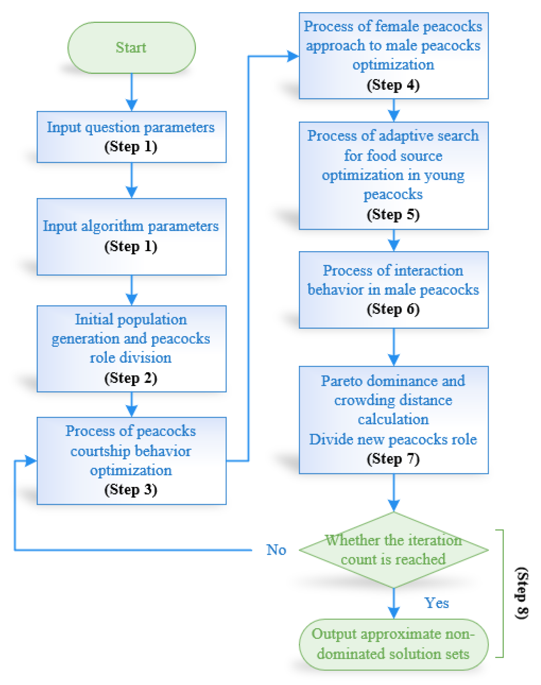
4.7. Algorithm Framework

In this section, we present the comprehensive framework of IPOA, integrating the core concepts discussed earlier. The algorithm consists of the following steps:

Step 1: Input algorithm parameters, including population size (Nsize), maximum iteration count (Maxit), number of stochastic simulations (T), Cv, and P_m.

Step 2: Calculate the objective function values for the initial population and perform the division of roles among the peafowls.

Step 3: Execute the optimization process for peafowls’ courtship behavior.

Step 4: Execute the optimization process for female peafowls.

Step 5: Execute the optimization process for peafowl chicks.

Step 6: Execute the interaction behavior process for male peafowls.

Step 7: After the optimization process in steps 3–6, we obtain optimized male peacocks, female peacocks, and peafowl chicks. Then, we merge them and perform Pareto dominance and crowding distance calculations on the optimized peacock population. Through these calculations, we sort the optimized peacock population and reassign roles to the peacocks.

Step 8: Check if the maximum iteration count has been reached. If it has, terminate the algorithm and output the approximate non-dominated solutions obtained by IPOA. If not, return to Step 3.

Finally, Figure 6 presents the overall flowchart of the algorithm, providing a visual representation of the algorithm’s sequence of steps and interactions.

5. Case Study

In this section, we present a case study focusing on a specific induced draft fan to demonstrate the effectiveness of our developed model and algorithm. We begin by calibrating the parameters of IPOA, which is a crucial step in solving problems using metaheuristic algorithms (Section 5.1). Subsequently, we solve the case, perform an analysis (Section 5.2), and compare the results with other advanced algorithms using multiple classic multi-objective evaluation metrics to showcase the effectiveness of IPOA (Section 5.3).

5.1. IPOA Parameter Calibration

As discussed in Section 4, IPOA consists of six parameters: Cv, Pm, Nsize, Maxit, Ee(1), and T. Based on a thorough analysis of the literature and preliminary experiments [7,11], we set the value of T to 1000. For the remaining parameters, we employ the Taguchi experimental method for calibration [44]. This method involves designing orthogonal arrays for conducting experiments and collecting and analyzing data to determine the optimal combination of operational parameters [45,46]. The Taguchi experimental method enables us to achieve favorable outcomes while utilizing computational resources efficiently, making it a widely adopted approach for parameter calibration. By employing the Taguchi experimental method, we can identify the best parameter combination within the given levels, ensuring effective results for IPOA.

Based on the literature analysis and preliminary experiments [1,3,5,8,12,38], we assigned four levels to each parameter in the IPOA, as presented in

Table 1. IPOA parameters and their reference values.

Parameters	Level 1	Level 2	Level 3	Level 4
Ee(1)	8	10	12	13
Nsize	30	40	50	60
Maxit	50	60	80	100
Cv	1	2	3	4
Pm	0.015	0.016	0.017	0.018

. These papers provide effective solutions to the disassembly problem and have been tested on a variety of problems using POA, and we initially determined the parameter ranges based on these papers and pre-experiments. Subsequently, we conducted further experiments to categorize the parameter ranges into different tiers and perform the subsequent parameter-calibration process. This approach allows for a comprehensive exploration of the parameter space and the assessment of the impact of different parameter settings on the experimental results.

According to the recommended Taguchi experimental method, we used the L16 orthogonal array for analysis. In addition, we used the Relative Percent Difference (RPD) to measure the performance of each parameter combination in each experiment. The calculation formula for RPD is shown in Equation (9). The experimental results are presented in

Table 2. Taguchi experiment RPD results.

Number: No.	Ee(1)	Nsize	Maxit	Cv	Pm	RPD
1	1	1	1	1	1	0.10661497
2	1	2	2	2	2	0.06577628
3	1	3	3	3	3	0.06812353
4	1	4	4	4	4	0.1340011
5	2	1	2	3	4	0.11658152
6	2	2	1	4	3	0.07820504
7	2	3	4	1	2	0.05479105
8	2	4	3	2	1	0
9	3	1	3	4	2	0.13238644
10	3	2	4	3	1	0.15900161
11	3	3	1	2	4	0.14063142
12	3	4	2	1	3	0.12227785
13	4	1	4	2	3	0.08530638
14	4	2	3	1	4	0.10210334
15	4	3	2	4	1	0.05515432
16	4	4	1	3	2	0.10953662

.

$$RPD=\frac{Al{g}_{Sol}-Mi{n}_{Sol}}{Mi{n}_{Sol}}$$

(9)

where $Mi{n}_{Sol}$ is the minimum value from the algorithm in all the experiments and $Al{g}_{Sol}$ is the value from the algorithm in each experiment.

Following the calculation of RPD for each parameter combination, we derived the average RPD for each factor level in its corresponding experimental combination. A smaller RPD value signifies better performance. The comprehensive experimental results are presented in

Table 3. Taguchi experiment results.

	Ee(1)	Nsize	Maxit	Cv	Pm
Level 1	0.093628970	0.110222328	0.108747013	0.096446803	0.080192725
Level 2	0.062394403	0.101271568	0.089947493	0.072928520	0.090622598
Level 3	0.138574330	0.079675080	0.075653328	0.113310820	0.088478200
Level 4	0.088025165	0.091453893	0.108275035	0.099936725	0.123329345

(Best value in bold).

5.2. Results and Analyses

After the parameter-calibration process, we determined the following parameter values: Ee(1) = 10, Nsize = 50, Maxit = 80, Cv = 2, tt = U (2,3), td = U (1,2) and Pm = 0.015. The other problem parameters are listed in

Table 4. Case study information.

Order	Name	Direction	Tool	Disassembly Time/s	Priority	Difficulty
1	Shell	+z	1	U (8,11)	0	0.2
2	Coupling	+z	1	U (5,7)	1	0.1
3	Duct expansion joint	+z	3	U (4,6)	0	0.15
4	Duct bolts	+z	3	U (2,3)	0	0
5	Duct Screws	−y	4	U (2,3)	0	0
6	Blower	+y	1	U (7,9)	1	0.3
7	Inlet vane guide device core	+z	2	U (15,16)	1	0.15
8	Intermediate connecting shaft short shaft tube	−y	1	U (11,13)	1	0.25
9	Impeller pressure plate bolts	−y	3	U (3,5)	0	0.1
10	Impeller	+y	4	U (7,8)	1	0.2
11	Bearing	−x	1	U (11,12)	1	0.2
12	Adjustable inlet guide vane	−x	1	U (10,13)	0	0.1
13	Outlet guide vane	−x	3	U (24,26)	0	0.2
14	Oil tank	−z	3	U (7,9)	1	0.3
15	Lube oil pump	+z	3	U (10,11)	1	0.15
16	Circulating cooling pump	+y	1	U (11,13)	0	0.15
17	Oil tank level meter	+y	2	U (5,6)	0	0
18	Oil tank thermometer	+y	2	U (8,9)	1	0
19	Lube oil line	+z	1	U (5,6)	0	0
20	Control oil line	+z	2	U (5,6)	0	0
21	Lubrication oil pressure gauge	+x	2	U (8,9)	1	0
22	Control oil pressure gauge	+x	1	U (9,12)	0	0

. In Table 4, we use x, y, and z to represent directions and numbers to represent tools. The disassembly mixed graph is illustrated in Figure 7.

The results of IPOA after one run are shown in

Table 5. Non-dominated solution sets obtained by IPOA.

Order	Schemes	f1	f2
1	3,22,11,12,13,14,10,18,5,19,21,15,4,20,6,16,17,1,7,8,9	233.54	114
2	10,14,11,15,3,5,18,2,19,4,12,6,7,8,22,17,13,16,9,1,21,20	247.36	85
3	2,11,14,10,3,1,18,19,15,5,21,4,6,22,12,7,8,17,9,16,13,20	258.86	83
4	11,10,14,2,15,3,22,13,18,4,5,1,16,6,12,19,7,20,21,8,9,17	233.65	94
5	14,22,10,1,2,11,13,12,3,4,18,15,19,5,17,20,21,16,6,7,8,9	232.26	115
6	2,22,11,12,1,13,14,10,18,17,3,19,20,21,5,4,15,16,6,7,8,9	230.33	119
7	14,2,11,22,18,15,3,10,4,12,19,5,6,1,7,16,8,9,13,21,20,17	247.00	90
8	22,14,10,3,15,11,18,2,16,19,4,5,6,21,17,7,20,8,9,1,12,13	245.14	92
9	2,10,11,3,14,15,13,5,18,4,12,6,7,8,22,17,16,19,1,21,20,9	251.12	85
10	10,2,11,14,17,15,3,1,16,18,19,21,20,4,5,6,7,13,22,12,8,9	245.52	92

.

Based on the results presented in Table 5, it is evident that there exists a trade-off relationship between the two objective functions. As f₁ decreases, f₂ exhibits a significant increase. This requires decision-makers to make trade-offs based on their priorities. For instance, if the objective is to minimize f₁, Solution 6 can be chosen. Conversely, if minimizing f₂ is the goal, Solution 9 is the preferred option. Solutions 1, 5, and 6 offer a relatively balanced trade-off between the two objectives. The availability of these ten solutions provides decision-makers with a wide range of options in an uncertain environment, thereby reducing decision costs and addressing uncertainties in the decomposition process. This ultimately enhances the effectiveness of equipment maintenance.

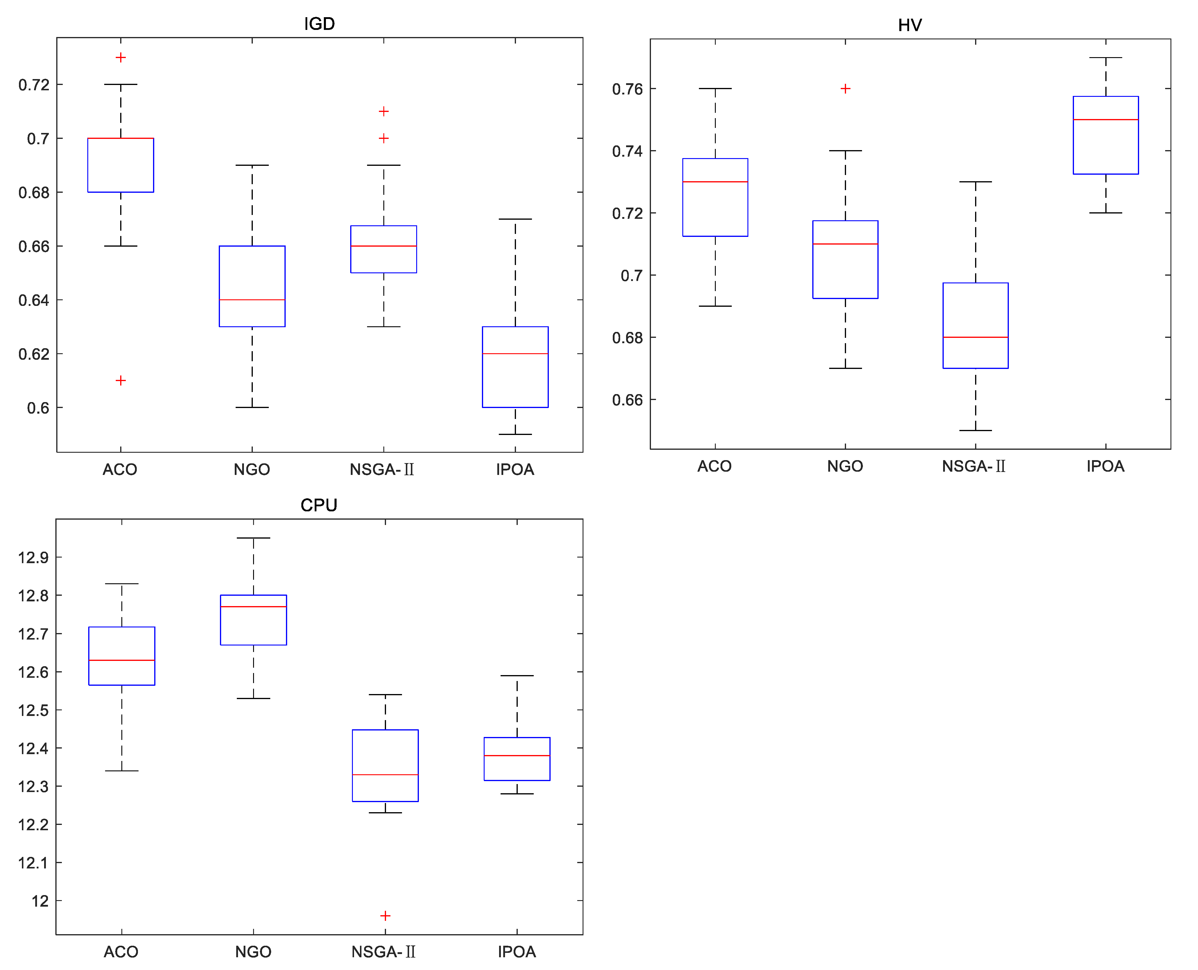
5.3. Comparison with Other Advanced Algorithms

To validate the effectiveness of IPOA, we compared its performance with other advanced algorithms, namely ant colony optimization algorithm (ACO) [47], NGO [21], and improved NSGA-II [48], which have been recently developed and customized for the decomposition problem, exhibiting promising performance. The comprehensive performance of these algorithms was evaluated using three classic multi-objective metrics: Inverted Generational Distance (IGD), Hypervolume (HV), and CPU time.

IGD measures the average distance between the solution set generated by the algorithm and the true Pareto front. A smaller IGD value indicates that the algorithm’s solution set is closer to the true Pareto front.

HV quantifies the size of the hypervolume occupied by the solution set generated by the algorithm. A larger HV value indicates that the algorithm’s solution set is closer to the true Pareto front in the objective space and exhibits a better distribution.

CPU time represents the total computation time required by the algorithm. A shorter CPU time generally indicates a faster execution speed of the algorithm.

To ensure fairness, we utilized the Taguchi method to determine the optimal parameters for each algorithm. We adopted the same encoding method and stochastic simulation strategy for all algorithms. To save computational resources, we set the number of stochastic simulations to 1 and used the data used in the first algorithm run for subsequent algorithm runs. Considering the inherent randomness of metaheuristic algorithms, each algorithm was executed fifteen times, and the average results are presented in

Table 6. Algorithms comparison results.

Algorithms	IGD	HV	CPU/s
ACO	0.69	0.73	12.63
NGO	0.64	0.71	12.75
NSGA-II	0.66	0.68	12.33
IPOA	0.62	0.75	12.39

. The statistical analysis results are displayed in Figure 8.

Based on the data from Table 6 and Figure 8, IPOA shows high performance in the HV and IGD metrics. Despite having a medium CPU time compared with other algorithms, the advantageous performance of IPOA in other evaluative metrics can offset this shortcoming. In addition, while NSGA-II records the shortest CPU time of the group, IPOA stands superior in terms of the quality metric results. The box-plot lengths in the statistical data highlight IPOA’s stability across the mentioned metrics. In conclusion, the evidence substantiates IPOA’s efficacy as an algorithm for addressing DSP problems.

6. Conclusions and Future Work

DSP is a critical technique employed to optimize the maintenance process of industrial equipment. By effectively planning the disassembly sequence, maintenance efficiency can be enhanced, downtime can be minimized [21], and equipment performance and reliability can be maintained for future operations.

In practical industrial environments, equipment disassembly often encounters various challenges and uncertainties, such as part dependencies, complex equipment structures, and resource constraints [49]. These factors contribute to the complexity and difficulty of DSP, necessitating comprehensive considerations to devise the optimal disassembly plan.

To address these challenges, this paper proposes a stochastic optimization-based DSP problem and presents an IPOA specifically designed for DSP problems. IPOA integrates several novel mechanisms to identify optimal or near-optimal disassembly sequences. Through flexible adjustments and collaborations, IPOA effectively searches for solution sequences that fulfill maintenance requirements.

The application of this improved DSP solution has yielded positive results in practical scenarios. It not only enhances the efficiency of maintenance and the quality of equipment but also reduces production downtime, maximizes resource utilization, and ensures selected disassembly sequences conform to workflow and safety standards.

As technology advances and research progresses, DSP will continue to evolve, offering more innovative solutions for industrial equipment maintenance. The study presented in this paper contributes to addressing challenges in industrial equipment maintenance processes, ultimately improving overall production efficiency and equipment reliability.

While this paper has made significant contributions to DSP problems in uncertain environments, there are still numerous avenues for future exploration. For instance, incorporating additional objective functions in the modeling process [50], developing more uncertainty-solving methods, and extending the research presented here to other disassembly problems [51], such as disassembly-line balancing and robot-disassembly-sequence planning, represent crucial directions for future investigation [52]. Finally, for future research on our IPOA, efforts could be focused on enhancing the efficiency and simplicity of the operators while also making well-considered decisions about the number of stochastic simulations to effectively conserve computational resources.

References

1. Tian, G.; Zhang, C.; Fathollahi-Fard, A.M.; Li, Z.; Zhang, C.; Jiang, Z. An enhanced social engineering optimizer for solving an energy-efficient disassembly line balancing problem based on bucket brigades and cloud theory. IEEE Trans. Ind. Inform. 2022, 19, 7148–7159. [Google Scholar] [CrossRef]
2. Agrawal, S.; Tiwari, M.K. A collaborative ant colony algorithm to stochastic mixed-model U-shaped disassembly line balancing and sequencing problem. Int. J. Prod. Res. 2008, 46, 1405–1429. [Google Scholar] [CrossRef]
3. Tian, G.; Ren, Y.; Feng, Y.; Zhou, M.; Zhang, H.; Tan, J. Modeling and planning for dual-objective selective disassembly using AND/OR graph and discrete artificial bee colony. IEEE Trans. Ind. Inform. 2018, 15, 2456–2468. [Google Scholar] [CrossRef]
4. Aghajani, M.; Ghodsi, R.; Javadi, B. Balancing of robotic mixed-model two-sided assembly line with robot setup times. Int. J. Adv. Manuf. Technol. 2014, 74, 1005–1016. [Google Scholar] [CrossRef]
5. Bentaha, M.L.; Dolgui, A.; Battaia, O.; Riggs, R.J.; Hu, J. Profit-oriented partial disassembly line design: Dealing with hazardous parts and task processing times uncertainty. Int. J. Prod. Res. 2018, 56, 7220–7242. [Google Scholar] [CrossRef]
6. Cui, X.S.; Guo, X.W.; Zhou, M.C.; Wang, J.; Qin, S.; Qi, L. Discrete whale optimization algorithm for disassembly line balancing with carbon emission constraint. IEEE Robot. Autom. Lett. 2023, 8, 3055–3061. [Google Scholar] [CrossRef]
7. Fu, Y.; Tian, G.; Fathollahi-Fard, A.M.; Ahmadi, A.; Zhang, C. Stochastic multi-objective modelling and optimization of an energy-conscious distributed permutation flow shop scheduling problem with the total tardiness constraint. J. Clean. Prod. 2019, 226, 515–525. [Google Scholar] [CrossRef]
8. Guo, X.; Zhou, M.; Abusorrah, A.; Alsokhiry, F.; Sedraoui, K. Disassembly sequence planning: A survey. IEEE/CAA J. Autom. Sin. 2020, 8, 1308–1324. [Google Scholar] [CrossRef]
9. Hui, W.; Dong, X.; Guanghong, D. A genetic algorithm for product disassembly sequence planning. Neurocomputing 2008, 71, 2720–2726. [Google Scholar] [CrossRef]
10. Deb, K.; Pratap, A.; Agarwal, S.; Meyarivan, T. A fast and elitist multiobjective genetic algorithm: NSGA-II. IEEE Trans. Evol. Comput. 2002, 6, 182–197. [Google Scholar] [CrossRef]
11. Ehteram, M.; Salih, S.Q.; Yaseen, Z.M. Efficiency evaluation of reverse osmosis desalination plant using hybridized multilayer perceptron with particle swarm optimization. Environ. Sci. Pollut. Res. 2020, 27, 15278–15291. [Google Scholar] [CrossRef] [PubMed]
12. Fang, Y.L.; Ming, H.; Li, M.Q.; Liu, Q.; Pham, D.T. Multi-objective evolutionary simulated annealing optimisation for mixed-model multi-robotic disassembly line balancing with interval processing time. Int. J. Prod. Res. 2020, 58, 846–862. [Google Scholar] [CrossRef]
13. Guo, X.W.; Liu, S.X.; Zhou, M.C.; Tian, G. Disassembly sequence optimization for large-scale products with multiresource constraints using scatter search and petri nets. IEEE Trans. Cybern. 2016, 46, 2435–2446. [Google Scholar] [CrossRef] [PubMed]
14. Gao, Y.C.; Wang, Q.R.; Feng, Y.X.; Zheng, H.; Zheng, B.; Tan, J. An energy-saving optimization method of dynamic scheduling for disassembly line. Energies 2018, 11, 1261. [Google Scholar] [CrossRef]
15. Zhou, Z.; Liu, J.; Pham, D.T.; Xu, W.; Ramirez, F.J.; Ji, C.; Liu, Q. Disassembly sequence planning: Recent developments and future trends. Proc. Inst. Mech. Eng. Part B J. Eng. Manuf. 2019, 233, 1450–1471. [Google Scholar] [CrossRef]
16. Tian, G.; Zhou, M.; Chu, J. A chance constrained programming approach to determine the optimal disassembly sequence. IEEE Trans. Autom. Sci. Eng. 2013, 10, 1004–1013. [Google Scholar] [CrossRef]
17. Goksoy Kalaycilar, E.; Batun, S.; Azizoğlu, M. A stochastic programming approach for the disassembly line balancing with hazardous task failures. Int. J. Prod. Res. 2022, 60, 3237–3262. [Google Scholar] [CrossRef]
18. Yu, D.; Zhang, X.; Tian, G.; Jiang, Z.; Liu, Z.; Qiang, T.; Zhan, C. Disassembly Sequence Planning for Green Remanufacturing Using an Improved Whale Optimisation Algorithm. Processes 2022, 10, 1998. [Google Scholar] [CrossRef]
19. Zhang, C.; Fathollahi-Fard, A.M.; Li, J.; Tian, G.; Zhang, T. Disassembly sequence planning for intelligent manufacturing using social engineering optimizer. Symmetry 2021, 13, 663. [Google Scholar] [CrossRef]
20. Wu, P.; Wang, H.; Li, B.; Fu, W.; Ren, J.; He, Q. Disassembly sequence planning and application using simplified discrete gravitational search algorithm for equipment maintenance in hydropower station. Expert Syst. Appl. 2022, 208, 118046. [Google Scholar] [CrossRef]
21. Zhan, C.; Zhang, X.; Tian, G.; Pham, D.T.; Ivanov, M.; Aleksandrov, A.; Fu, C.; Zhang, J.; Wu, Z. Environment-oriented disassembly planning for end-of-life vehicle batteries based on an improved northern goshawk optimisation algorithm. Environ. Sci. Pollut. Res. 2023, 30, 47956–47971. [Google Scholar] [CrossRef]
22. Mahmoudi Motahar, M.; Hosseini Nourzad, S.H. A hybrid method for optimizing selective disassembly sequence planning in adaptive reuse of buildings. Eng. Constr. Archit. Manag. 2022, 29, 307–332. [Google Scholar] [CrossRef]
23. Sun, X.; Guo, S.; Guo, J.; Du, B.; Tang, H. An improved multi-objective evolutionary algorithm for multiple-target asynchronous parallel selective disassembly sequence planning. Proc. Inst. Mech. Eng. Part B J. Eng. Manuf. 2022, 237, 1553–1569. [Google Scholar] [CrossRef]
24. Chen, Z.; Li, L.; Zhao, F.; Sutherland, J.W.; Yin, F. Disassembly sequence planning for target parts of end-of-life smartphones using Q-learning algorithm. Procedia CIRP 2023, 116, 684–689. [Google Scholar] [CrossRef]
25. Ji, J.; Wang, Y. Selective disassembly sequence optimization based on the improved immune algorithm. Robot. Intell. Autom. 2023, 43, 96–108. [Google Scholar] [CrossRef]
26. Kheder, M.; Trigui, M.; Aifaoui, N. Disassembly sequence planning based on a genetic algorithm. Proc. Inst. Mech. Eng. Part C J. Mech. Eng. Sci. 2015, 229, 2281–2290. [Google Scholar] [CrossRef]
27. Fu, Y.; Zhou, M.; Guo, X.; Qi, L.; Sedraoui, K. Multiverse optimization algorithm for stochastic biobjective disassembly sequence planning subject to operation failures. IEEE Trans. Syst. Man Cybern. Syst. 2021, 52, 1041–1051. [Google Scholar] [CrossRef]
28. Liang, P.; Fu, Y.; Ni, S.; Zheng, B. Modeling and optimization for noise-aversion and energy-awareness disassembly sequence planning problems in reverse supply chain. Environ. Sci. Pollut. Res. 2021, 15, 748–760. [Google Scholar] [CrossRef]
29. Tian, G.; Zhou, M.; Li, P. Disassembly sequence planning considering fuzzy component quality and varying operational cost. IEEE Trans. Autom. Sci. Eng. 2017, 15, 748–760. [Google Scholar] [CrossRef]
30. Kim, H.W.; Park, C.; Lee, D.H. Selective disassembly sequencing with random operation times in parallel disassembly environment. Int. J. Prod. Res. 2018, 56, 7243–7257. [Google Scholar] [CrossRef]
31. Liang, P.; Fu, Y.; Guo, X.; Qi, L. Stochastic multi-product disassembly sequence planning. In Proceedings of the 2021 IEEE 17th International Conference on Automation Science and Engineering (CASE), Lyon, France, 23–27 August 2021; pp. 1201–1206. [Google Scholar]
32. Yeh, W.C.; Lin, C.M.; Wei, S.C. Disassembly sequencing problems with stochasticprocessing time using simplified swarm optimization. Int. J. Innov. Manag. Technol. 2012, 3, 226. [Google Scholar]
33. Erel, E.; Sabuncuoglu, I.; Sekerci, H. Stochastic assembly line balancing using beam search. Int. J. Prod. Res. 2005, 43, 1411–1426. [Google Scholar] [CrossRef]
34. Mosadegh, H.; Ghomi, S.F.; Süer, G.A. Stochastic mixed-model assembly line sequencing problem: Mathematical modeling and Q-learning based simulated annealing hyper-heuristics. Eur. J. Oper. Res. 2020, 282, 530–544. [Google Scholar] [CrossRef]
35. Sakiani, R.; Ghomi, S.F.; Zandieh, M. Multi-objective supply planning for two-level assembly systems with stochastic lead times. Comput. Oper. Res. 2012, 39, 1325–1332. [Google Scholar] [CrossRef]
36. Fu, Y.; Zhou, M.; Guo, X.; Qi, L. Stochastic multi-objective integrated disassembly-reprocessing-reassembly scheduling via fruit fly optimization algorithm. J. Clean. Prod. 2021, 278, 123364. [Google Scholar] [CrossRef]
37. Wolpert, D.H.; Macready, W.G. No free lunch theorems for optimization. IEEE Trans. Evol. Comput. 1997, 1, 67–82. [Google Scholar] [CrossRef]
38. Wang, J.; Yang, B.; Chen, Y.; Zeng, K.; Zhang, H.; Shu, H.; Chen, Y. Novel phasianidae inspired peafowl (Pavo muticus/cristatus) optimization algorithm: Design, evaluation, and SOFC models parameter estimation. Sustain. Energy Technol. Assess. 2022, 50, 101825. [Google Scholar] [CrossRef]
39. Fathollahi-Fard, A.M.; Woodward, L.; Akhrif, O. Sustainable distributed permutation flow-shop scheduling model based on a triple bottom line concept. J. Ind. Inf. Integr. 2021, 24, 100233. [Google Scholar] [CrossRef]
40. Chen, J.C.; Chen, Y.Y.; Chen, T.L.; Yang, Y.C. An adaptive genetic algorithm-based and AND/OR graph approach for the disassembly line balancing problem. Eng. Optim. 2022, 54, 1583–1599. [Google Scholar] [CrossRef]
41. Fathollahi-Fard, A.M.; Hajiaghaei-Keshteli, M.; Tavakkoli-Moghaddam, R. The social engineering optimizer (SEO). Eng. Appl. Artif. Intell. 2018, 72, 267–293. [Google Scholar] [CrossRef]
42. Guo, X.; Zhang, Z.; Qi, L.; Liu, S.; Tang, Y.; Zhao, Z. Stochastic hybrid discrete grey wolf optimizer for multi-objective disassembly sequencing and line balancing planning in disassembling multiple products. IEEE Trans. Autom. Sci. Eng. 2021, 19, 1744–1756. [Google Scholar] [CrossRef]
43. Tian, G.; Liu, Y.; Tian, Q.; Chu, J. Evaluation model and algorithm of product disassembly process with stochastic feature. Clean Technol. Environ. Policy 2012, 14, 345–356. [Google Scholar] [CrossRef]
44. Fathollahi-Fard, A.M.; Ahmadi, A.; Karimi, B. Sustainable and Robust Home Healthcare Logistics: A Response to the COVID-19 Pandemic. Symmetry 2022, 14, 193. [Google Scholar] [CrossRef]
45. Bernal, E.; Lagunes, M.L.; Castillo, O.; Soria, J.; Valdez, F. Optimization of type-2 fuzzy logic controller design using the GSO and FA algorithms. Int. J. Fuzzy Syst. 2021, 23, 42–57. [Google Scholar] [CrossRef]
46. Fathollahi-Fard, A.M.; Tian, G.; Ke, H.; Fu, Y.; Wong, K.Y. Efficient Multi-objective Metaheuristic Algorithm for Sustainable Harvest Planning Problem. Comput. Oper. Res. 2023, 158, 106304. [Google Scholar] [CrossRef]
47. Xing, Y.; Wu, D.; Qu, L. Parallel disassembly sequence planning using improved ant colony algorithm. Int. J. Adv. Manuf. Technol. 2021, 113, 2327–2342. [Google Scholar] [CrossRef]
48. Ren, Y.; Zhang, C.; Zhao, F.; Xiao, H.; Tian, G. An asynchronous parallel disassembly planning based on genetic algorithm. Eur. J. Oper. Res. 2018, 269, 647–660. [Google Scholar] [CrossRef]
49. Tian, G.; Zhang, X.; Fathollahi-Fard, A.M.; Jiang, Z.; Zhang, C.; Yuan, G.; Pham, D.T. Hybrid evolutionary algorithm for stochastic multiobjective disassembly line balancing problem in remanufacturing. Environ. Sci. Pollut. Res. 2023, 1–16. [Google Scholar] [CrossRef]
50. Tian, G.; Zhang, L.; Fathollahi-Fard, A.M.; Kang, Q.; Li, Z.; Wong, K.Y. Addressing a collaborative maintenance planning using multiple operators by a multi-objective Metaheuristic algorithm. IEEE Trans. Autom. Sci. Eng. 2023. [Google Scholar] [CrossRef]
51. Wang, W.; Tian, G.; Zhang, H.; Li, Z.; Zhang, L. A hybrid genetic algorithm with multiple decoding methods for energy-aware remanufacturing system scheduling problem. Robot. Comput.-Integr. Manuf. 2023, 81, 102509. [Google Scholar] [CrossRef]
52. Xu, K.; Fan, Y.; Zhu, C.; Tian, G.; Hu, L. Multiple Spatiotemporal Broad Learning for Real-Time Temperature Estimation of Lithium-Ion Batteries. Ind. Eng. Chem. Res. 2023, 62, 6251–6261. [Google Scholar] [CrossRef]
Figure 1. Disassembled mixed graph.
Processes 11 02462 g001
Figure 2. Peafowl courtship behavior.
Processes 11 02462 g002
Figure 3. Adaptive behavior of female peafowls in proximity.
Processes 11 02462 g003
Figure 4. Adaptive search behavior of peafowl chick.
Processes 11 02462 g004
Figure 5. Interactive behavior among male peafowls.
Processes 11 02462 g005
Figure 6. IPOA general framework.
Processes 11 02462 g006
Figure 7. Disassembly mixed graph information.
Processes 11 02462 g007
Figure 8. Algorithms comparison results boxplot (+ represents outliers).
Processes 11 02462 g008