Remote Monitoring the Parameters of Interest in the ¹⁸O Isotope Separation Technological Process

Abstract

This manuscript presents the remote monitoring of the main parameters in the ¹⁸O isotope separation technological process. It proposes to monitor the operation of the five cracking reactors in the isotope production system, respectively, the temperature in the preheating furnaces, the converter reactors and the cracking reactors. In addition, it performs the monitoring of the two separation columns from the separation cascade structure, respectively, the concentrations of the produced ¹⁸O isotope and the input nitric oxides flows. Even if the production process is continuously monitored by teams of operators, the professionals who designed the technical process and those who can monitor it remotely have the possibility to intervene with the view of making the necessary adjustments. Based on the processing of experimental data, which was gathered from the actual plant, the proposed original model of the separation cascade functioning was developed. The process computer from the monitoring system structure runs the proposed mathematical model in parallel with the real plant and estimates several signal values, which are essential to be known by the operators in order to make the appropriate decisions regarding the plant operation. The separation process associated with the final separation column from the separation cascade structure is modeled as a fractional-order process with variable and adjustable differentiation order, which represents another original aspect. Neural networks have been employed in order to implement the proposed mathematical model. The accuracy, validity and efficiency in the operation of the proposed mathematical model is demonstrated through the simulation results presented in the final part of the manuscript.

1. Introduction

To identify remote monitoring and control solutions in many domains so as to minimize the losses in the industrial sector [1].

The importance of stable isotopes in recent years has increased substantially [2,3,4,5,6]. As marker elements, these isotopes have proven to be a very advantageous tool in a number of fields, such as chemistry, biology, medicine, agriculture, archaeology and others [2,3,4,5].

In this regard, a productive pilot plant for isotope exchange between nitrogen oxides and nitric acid solution and water has been built at INCDTIM Cluj-Napoca. The ¹⁸O isotope plant uses NO and NO₂ residuals from the ¹⁵N nitrogen isotope plant; the method is by isotope exchange reactions [7,8].

In order to make decisions that will not affect the separation process, the ¹⁸O separation productive installation must be supervised from a distance due to its response time and time constant of hundreds of hours [8]. The professionals who designed the technical process and who may monitor it remotely have the possibility to intervene to make the necessary adjustments [9,10,11,12,13,14].

This manuscript aims to approach the aspect mentioned above, i.e., remote monitoring of isotopic exchange processes with applications to the separation of the heavy isotope of oxygen ¹⁸O through isotopic exchange reaction between nitrogen oxides and nitric acid and water solution, on a productive pilot plant at INCDTIM Cluj-Napoca [15,16]. In addition, the study aims to suggest a mathematical model that describes the operation of the separation plant. By using this model along with simulation, important information can be provided to the operators of the separation cascade.

The diagram of a process monitoring interface was elaborated, and the physical accomplishment of an experimental board for the implementation of an interface aimed at “reading” these parameters and transmitting them to the computer used in the monitoring process [17,18,19].

A process monitoring program runs on the aforementioned device. Based on the values of the parameters, it can send E-Mails, SMS, and notification to the approved staff, emphasizing the modification of parameters during the operation of the productive installation. On the other hand, with the help of this program, knowledgeable personnel can interrogate the value of the respective parameters. A database includes users’ rights [19] and the name, phone number, e-mail, and contact address of all approved users from the system and options with rights in the system.

The modeling of ¹⁸O isotope separation processes has been approached in several articles from technical literature, but they propose linearized models which are valid only near particular working points [20]. Some other articles approach solutions for controlling the produced isotope concentration, which is also based on linearized models [21,22].

This study proposes an original method for the non-linear modeling of the separation process behavior, considering the fact that the technological process associated with the final separation column from the separation cascade structure is a fractional-order one [23]. With the view of efficiently implementing the process’s nonlinearities, artificial intelligence methods [24,25] are applied based on using neural networks [26].

The system’s identification techniques are classified into three categories: analytical identification, experimental identification and hybrid identification (in this case, the mathematical model structure is obtained by using analytical identification and the model’s structure parameters are identified using analytical identification).

The analytical identification is based on determining the systems of equations that governs the operation of the system, respectively, on the mathematical processing of the system’s equations in order to obtain a direct mathematical dependency between the input and the output signal. The main advantages of the analytical mathematical models are their high accuracy and validity due to the fact that they result directly from the system’s properties. Additionally, the main disadvantage of them is the fact that in the majority of cases, they have a high order, and they have to be simplified in order to be used in practice (partially losing the advantage of their high accuracy). Examples of several analytical models and of methods for their determination are presented in [27]. However, the technical literature is poor regarding the information in the domain of the analytical modeling of separation processes.

The experimental identification techniques of mathematical models are applied based on processing the experimental data obtained from the real processes. Their main advantages are the high validity (due to the fact that the result is based on real measurements) and the fact that, in general, they are obtained using more simple methods than in the case of analytical identification (from the mathematical perspective). Their main disadvantage is the fact that the corresponding experiments have to be organized (an aspect that introduces a lot of technological problems and additional costs), and they are not always technologically possible to be organized.

Examples of experimental identification methods applicable for modeling the linear processes, such as the tangent method, the Cohen–Coon method, the Strejc method, the method of successive logarithms or the decomposition method into simple elements, are presented in [28,29,30]. These methods generate continuous mathematical models. Additionally, methods for identifying the parametric mathematical models, such as the method of least squares, the instrumental variable method or the generalized method of least squares, are presented in [31,32]. However, they are limited regarding their application in the case of the nonlinear processes as the considered separation process. Methods for the identification of nonlinear systems, such as the state-dependent-parameter (SDP) estimation, are presented in [33,34].

However, in this manuscript, an alternative hybrid procedure of identification is applied. The proposed mathematical model structure is determined analytically, and also, some quantities as the separation function. In the same context, for obtaining the structure parameters of the proposed mathematical model, experimental identification is applied due to the availability of several types of experimental data (the process step type response and the experimentally determined dynamics of some important functions, such as the heights of equivalent theoretical plates). Additionally, in order to implement the proposed mathematical model nonlinearities and its fractional-order component, artificial intelligence (AI) techniques based on neural networks are used.

Modern approaches for nonlinear system identification have been proposed recently: nonlinear differential equations [35], Nonlinear Autoregressive Moving Average with Exogenous Inputs NARMAX models [36,37], neural networks [38,39], spline adaptive filters [40], deep state-space models parametric identification methods like hybrid synchronization, parameter fitting [41], etc.

Extended spatiotemporal equations, such as partial differential equations, coupled map lattices, or coupled ordinary differential equations, are used to model a variety of natural physical phenomena. Differential equations draw the attention of scientists and engineers because it is possible to create precise white-box models, which frequently have a well-established physical explanation. The concept of phase space, also known as “state space,” is crucial for understanding both discrete and continuous dynamical systems. It is an abstract mathematical construction with important applications in statistical mechanics to represent the time evolution of a dynamical system in geometric shape. This space has as many dimensions as the number of variables needed to define the instantaneous state of the system.

There has been an increasing demand in complex industries to develop reliable condition-monitoring techniques to monitor real-time system status and promote advanced optimization algorithms and resilient control methods to ensure the desired control and operation performance [42]. Recently, artificial intelligence, data-driven techniques, cyber-physical systems, and cloud and cognitive computation have further stimulated research and applications of monitoring, optimization, and control techniques [43].

There is a growing demand for temperature control of thermal processing systems. In [44], a novel slow-mode-based control approach was presented for multipoint temperature control systems, where the temperature differences and the transient responses can be regulated, ensuring the outputs of the fast modes follow that of the slow mode.

The first chapter represents an introduction to the topic discussed throughout the work.

In the second chapter, entitled “The modeling of the ¹⁸O isotope production process”, the mathematical modeling of the separation cascade behavior is made. Experimental data and the applied modeling procedures are also presented. Furthermore, the section highlights the main interconnections between the different subsystems from the proposed mathematical model structure.

The first part of the third chapter, entitled “Method of Implementing Remote Process Monitoring” focuses on several preliminaries regarding the usual management of a technological process with the help of the computer. The chapter continues with the presentation of modifications necessary for enabling the remote monitoring of the system [45]. The second part of this chapter refers to the specific solutions found for monitoring some “key” parameters in the functioning of the system for obtaining ¹⁸O isotopes by isotopic exchange reactions. Six logical parameters (ON/OFF) and six numerical parameters (temperatures) are illustrated [46,47,48,49]. The monitoring of temperatures in all the equipment operations from the separation cascade is very important in order to maintain the elementary separation factor of the ¹⁸O isotope (α) constant and to analyze its possible deviations near its nominal value.

Starting from their values, a specialist who has a good understanding of the process can figure out whether the operation proceeds normally or whether there are some anomalies that might lead to the compromise of the final result, along with a waste of raw materials and resources [50].

The fourth chapter, entitled “Results”, presents the obtained system, the interface for monitoring and the software for monitoring. For testing and simulating variations in the monitored parameters in the process, a panel with potentiometers and switches was made. The length of the cables was simulated with networks of resistors and capacitors. The power supply of the devices through these long wires was also tested. Additionally, the simulation results obtained by the simulation of the suggested mathematical model, which describes the separation cascade operation, are presented. Some interesting interpretations of these results are given.

The last chapter, “Conclusions and further developments”, presents both the outcomes of the research and suggests possibilities for developing this topic in the future.

From the mathematical perspective, the following theoretical goals are set for the current research:

• The determination of the structure of the original mathematical model, which describes the behavior of the approached separation cascade, considering that this process is a strong nonlinear fractional-order one.
• The determination of the analytical equations of the parameters associated with the separation cascade is usable for the model parametrization (for example, the separation functions or the steady-state values of the ¹⁸O isotope concentration at the top of the two separation columns from the separation cascade structure).
• The proposing of an original method for the simulation of the proposed fractional-order model in the context when the main disturbance which can occur in the process is the variation of the fractional differentiation order (associated with the fractional-order component of the model).
• Defining the structure of the neural networks used as AI techniques for having the possibility to simulate the proposed mathematical model (the neural networks are necessary to implement the nonlinear and the fractional-order components of the proposed mathematical model).
• The implementation of the proposed mathematical model functional diagram in which are highlighted the interconnections between the different components of the model.

The simulation of the proposed mathematical model is obtained in different relevant scenarios both in the case when the main disturbance occurs and when it does not occur in the system; an interesting aspect is represented by the simulation of the effect of the fractional differentiation order variation (associated to the fractional-order component of the proposed mathematical model).

2. The modeling of the ¹⁸O Isotope Production Process

2.1. Technological Description of the ¹⁸O Isotope Separation Cascade

The main elements of the considered ¹⁸O isotope separation cascade are presented in Figure 1.

Two separation columns are part of the framework of the separation cascade (the first separation column is marked as SC1, and the second separation column is marked as SC2. The height of SC1 is equal to that of SC2, more exactly h = 1000 cm. The supply of SC1 is made at its base with nitric oxides (NO, NO₂) (their concentration is equal to the natural abundance (Z₀ = 0.204%) of the ¹⁸O isotope) using the P1 pump, which circulates the F₁ flow. Additionally, the supply of SC2 with nitric oxides (having the concentration of the ¹⁸O isotope higher than its natural abundance and being obtained from the top of SC1) is made at its base. In this case, the P2 pump is used, which circulates the F₂ flow. The two input flows can be modified by variating the electrical supply of the two pumps (P1 and P2). The reflux systems (SC1RS and SC2RS) of the two separation columns make possible the correct operation of the separation cascade. The equipment from the structure of the reflux systems includes absorbers, arc-cracking reactors, and catalytic reactors. The supply flows with hydrogen (necessary for the production of the nitric acid solutions) of the two reflux systems, F_H1 and F_H2.

SC1 and SC2 are supplied at their tops with nitric acid solutions (the corresponding flows being F_NA1 and F_NA2). Inside the separation’s columns, the nitric oxides and the nitric acid circulate in counter-current, in a context where the contact between the two substances occurs. The contact makes possible the enrichment of the ¹⁸O isotope. The two separation columns’ usage of oblique parallel lines indicates that they include steel packing, which is used for a more efficient contact between the two mentioned substances that circulate in counter-current. The excesses of the hydrogen and nitrogen generated by the two reflux systems are evacuated with F_E1 and F_E2 flows. F_W is the waste flow (under the form of nitric acid solution) evacuated from the SC1 base.

The nitric oxides flow at the output from the two separation columns tops are F_NO1 and F_NO2. In this context, F_NO is the nitric oxide flow circulated from SC1 to SC2 (consequently, SC2 is supplied by SC1; more exactly, SC2 enriches the ¹⁸O isotope already enriched by SC1). Additionally, F_NA is the nitric acid flow circulated from SC2 to SC1, the same quantity of ¹⁸O isotope being returned from SC2 in SC1.

The product is extracted (in the production regime) from the tops of the two separation columns under the form of nitric acids, having an increased concentration of ¹⁸O isotope compared to its natural abundance. In the production regime, the two flows of the extracted product are F_P1 and F_P2. The second usually separation cascade operation regime is named total reflux regime (in this regime, the ¹⁸O isotope is enriched without extracting product, more exactly F_P1 = F_P2 = 0 L/h).

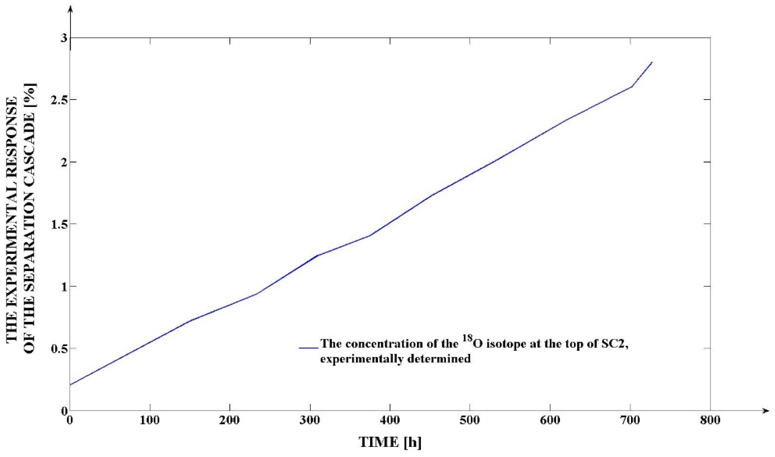
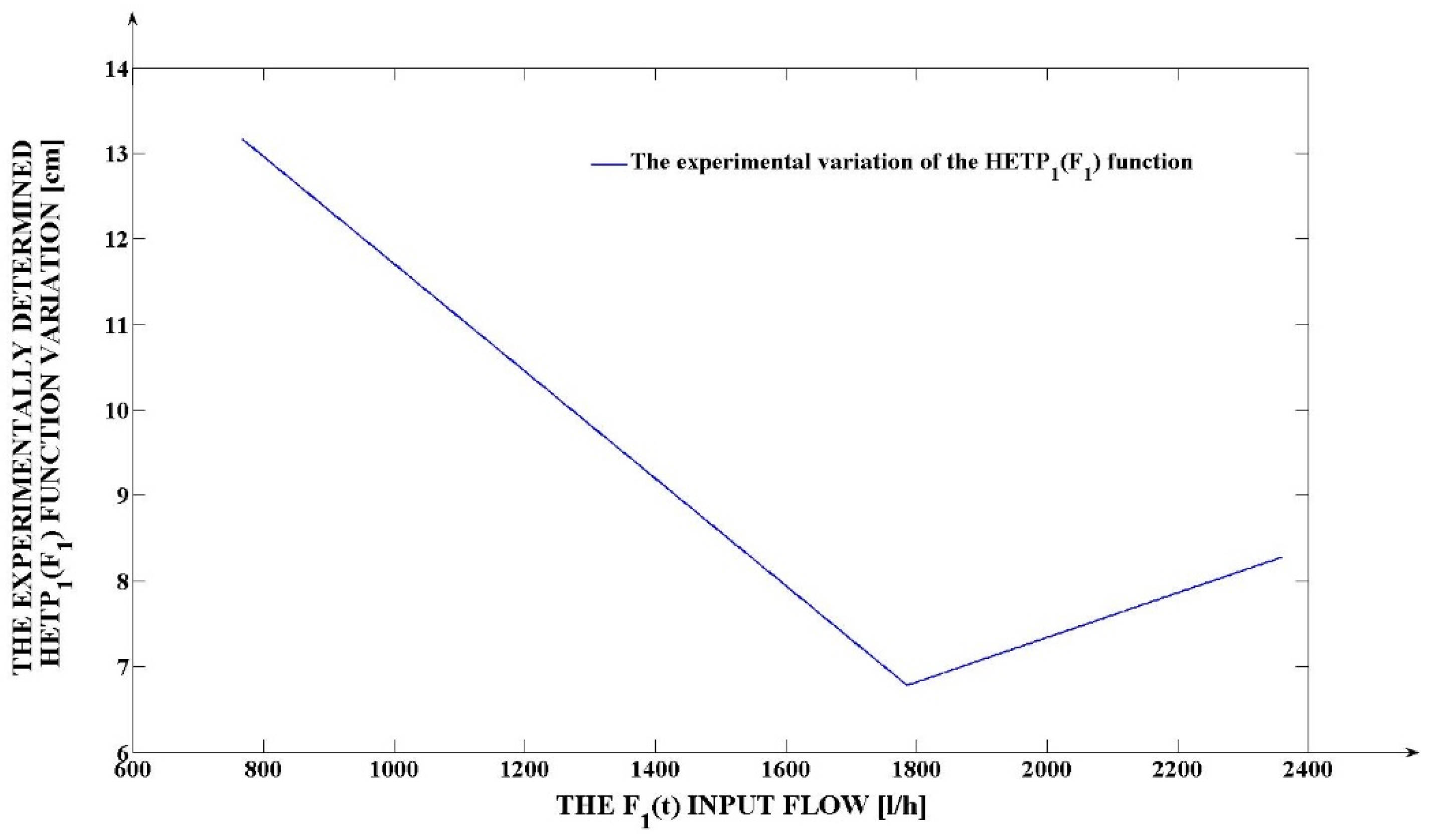
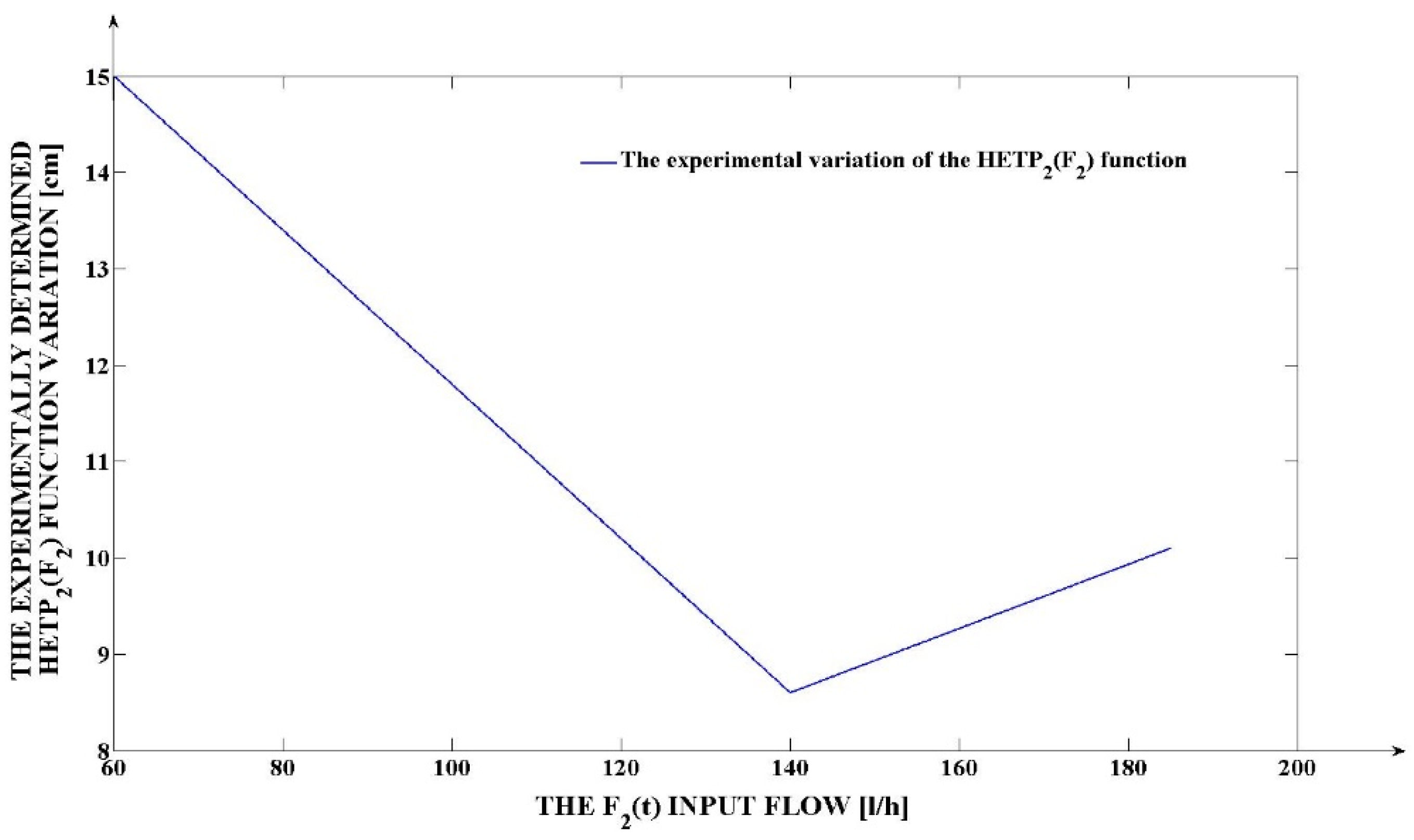
2.2. Experimental Results

The experimental data are obtained from the real separation cascade by making measurements both in the experimental regime and in the production regime. This manuscript approaches only the experimental results corresponding to the separation cascade operation in the total reflux regime. In this context, the modeling of the separation process is made for the case when the product is not extracted from the two separation columns (instead, it is only enriched).

The experimental open-loop step response of the separation cascade (and implicitly of SC2) is presented in Figure 2 for F₁ = 880 L/h and F₂ = 80 L/h (signals of step types).

The experiment was interrupted after 730 h due to a failure; the ¹⁸O isotope concentration did not reach the steady state value. However, the obtained response dynamics are relevant for the identification of the proposed mathematical model and for determining its structure parameters. As it was previously highlighted, the main output signal of the separation cascade is the same as the output signal from SC2 (¹⁸O isotope concentration at the top of SC2). The ¹⁸O isotope concentration at the SC1 top is a secondary output signal (it is not necessary to use the experimental response of SC1 for identifying the separation cascade mathematical model; the obtained ¹⁸O isotope concentration at the SC2 output is the effect of the entire plant operation (including SC1), of SC2). The sensor used for the ¹⁸O isotope concentration measurement is the mass spectrometer.

The second types of experimental results obtained from the separation cascade are the dynamics of the HETP (Height of Equivalent Theoretical Plate) functions, which are very important for the separation cascade modeling. The values of these functions are obtained by applying different values of the two input flows at the input of each separation column (SC1 and SC2). These experiments were made individually for each column (without being included in the separation cascade). For each input flow, using the measured, steady-state values of the ¹⁸O isotope concentrations at the top of each column, the associated HETP function values are computed based on the direct mathematical dependency between them. The experimental results are given in

Table 1. HETP experimental results.

No.	F1 [L/h]	HETP1 (F1) [cm]	F2 [L/h]	HETP2 (F2) [cm]
1	766.9	13.1	60.1	14.9
2	926.3	12.1	72.6	13.9
3	1085.7	11.1	85.1	12.9
4	1245.2	10.1	97.6	11.9
5	1404.6	9.1	110.1	10.9
6	1564.1	8.1	122.6	9.9
7	1642.2	7.6	128.7	9.5
8	1723.5	7.1	135.1	8.9
9	1785.7	6.7	140	8.6
10	1882.9	7	147.6	8.8
11	2042.4	7.4	160.1	9.2
12	2201.8	7.8	172.6	9.6
13	2359.7	8.2	185	10.1

.

In Figure 3 and Figure 4, the HETP₁(F₁) and HETP₂(F₂) functions are graphically represented. Figure 3 and Figure 4 show that the two HETP functions are nonlinear (they are linear on different domains, but they are not linear on the entire definition domain). From the elementary separation isotopes theory, it is known that the concentration of the produced ¹⁸O isotope has higher values when the associated HETP(F) has lower values; respectively, it has lower values when the corresponding HETP(F) has higher values. Consequently, for the minimum values of the graphs presented in Figure 3 and Figure 4, the highest values of the ¹⁸O isotope concentrations are obtained (at the tops of the two separation columns).

2.3. The Proposed Mathematical Model

The steady-state value of the ¹⁸O isotope concentration at the SC2 output (top) is given by the following equation [51,52,53,54,55,56,57,58]:

$${\mathrm{Z}}_{2\mathrm{s}\mathrm{t}}\left(\mathrm{t}\right)={\mathrm{Z}}_0·{{\mathsf{\alpha }}^{\frac{\mathrm{h}}{{\mathrm{H}\mathrm{E}\mathrm{T}\mathrm{P}}_1\left({\mathrm{F}}_1\right)}}·\mathsf{\alpha }}^{\frac{\mathrm{h}}{{\mathrm{H}\mathrm{E}\mathrm{T}\mathrm{P}}_2\left({\mathrm{F}}_2\right)}}$$

(1)

where α = 1.018 [-] is the elementary separation factor of the ¹⁸O isotope, Z₀ = 0.204% (its significance is explained previously in this section of the manuscript), the second factor of the right member shows the separation of SC1, and the third factor of the right member shows the separation of SC2. Additionally, (1) it can be rewritten under the form:

$${\mathrm{Z}}_{2\mathrm{s}\mathrm{t}}\left(\mathrm{t}\right)={\mathrm{Z}}_0·{{\mathsf{\alpha }}^{\frac{\mathrm{h}}{{\mathrm{H}\mathrm{E}\mathrm{T}\mathrm{P}}_1\left({\mathrm{F}}_1\right)}}·\mathsf{\alpha }}^{\frac{\mathrm{h}}{{\mathrm{H}\mathrm{E}\mathrm{T}\mathrm{P}}_2\left({\mathrm{F}}_2\right)}}={\mathrm{Z}}_0·{\mathsf{\alpha }}^{\frac{\mathrm{h}}{\frac{{\mathrm{H}\mathrm{E}\mathrm{T}\mathrm{P}}_1\left({\mathrm{F}}_1\right)·{\mathrm{H}\mathrm{E}\mathrm{T}\mathrm{P}}_2\left({\mathrm{F}}_2\right)}{{\mathrm{H}\mathrm{E}\mathrm{T}\mathrm{P}}_1\left({\mathrm{F}}_1\right)+{\mathrm{H}\mathrm{E}\mathrm{T}\mathrm{P}}_2\left({\mathrm{F}}_2\right)}}}$$

(2)

in which the following notation is made:

$${\mathrm{H}\mathrm{E}\mathrm{T}\mathrm{P}}_{\mathrm{e}}\left({\mathrm{F}}_1,{\mathrm{F}}_2\right)=\frac{{\mathrm{H}\mathrm{E}\mathrm{T}\mathrm{P}}_1\left({\mathrm{F}}_1\right)·{\mathrm{H}\mathrm{E}\mathrm{T}\mathrm{P}}_2\left({\mathrm{F}}_2\right)}{{\mathrm{H}\mathrm{E}\mathrm{T}\mathrm{P}}_1\left({\mathrm{F}}_1\right)+{\mathrm{H}\mathrm{E}\mathrm{T}\mathrm{P}}_2\left({\mathrm{F}}_2\right)}$$

(3)

The ${\mathrm{H}\mathrm{E}\mathrm{T}\mathrm{P}}_{\mathrm{e}}\left({\mathrm{F}}_1,{\mathrm{F}}_2\right)$ function represents the equivalent Height of Equivalent Theoretical Plate of the separation cascade.

An important problem for the plant operators is to obtain a certain imposed steady state value for the ¹⁸O isotope concentration at the SC2 output in the separation cascade open loop operation. The main difficulty, in this case, is the fact that the operators have to know exactly the values of the F₁(t) and F₂(t) input flows which have to be applied at the separation cascade input in order to obtain the imposed ¹⁸O isotope concentration at its output. A possible solution is to impose a certain value for the F₁(t) and to compute the appropriate value of F₂(t), which can be used for solving the mentioned problem. It is preferred to impose the F₁(t) flow due to the fact that (according to Table 1, respectively to Figure 3 and Figure 4) it has much higher values than F₂(t) (the limits of the F₁(t) variation domain are more than ten times bigger than the limits of the F₂(t) variation domain). In this context, by limiting the value of F₁(t), important energy consumption savings can be obtained. It is important to mention that analyzing the dynamics of the graphs from Figure 3 and Figure 4, in the case of each separation column and for a consistent domain of values, the same HETP(F) value can be obtained by applying two different flow values. If a certain F₁(t) value is imposed, then the corresponding HETP value will be constant, and the notation C = HETP₁(F_1imp) can be made, where C is the HETP₁ value if the imposed nitric oxides flow F_1imp is applied at the SC1 input. Considering, also, the imposed steady-state value of the ¹⁸O concentration at the SC2 output Z_stimp, the HETP₂(F₂) function can be determined from (2). Consequently, it results in that:

$${\mathrm{H}\mathrm{E}\mathrm{T}\mathrm{P}}_2\left({\mathrm{F}}_2\right)=\frac{\mathrm{h}·\mathrm{C}}{\mathrm{C}·\left[{\mathrm{l}\mathrm{o}\mathrm{g}}_{\mathsf{\alpha }}\left(\frac{{\mathrm{Z}}_{\mathrm{s}\mathrm{t}\mathrm{i}\mathrm{m}\mathrm{p}}}{{\mathrm{Z}}_0}\right)\right]-\mathrm{h}}$$

(4)

from which the appropriate value of F₂(t), in order to obtain Z_stimp, results:

$${\mathrm{F}}_2={\mathrm{H}\mathrm{E}\mathrm{T}\mathrm{P}}_2^{-1}\left(\frac{\mathrm{h}·\mathrm{C}}{\mathrm{C}·\left[{\mathrm{l}\mathrm{o}\mathrm{g}}_{\mathsf{\alpha }}\left(\frac{{\mathrm{Z}}_{\mathrm{s}\mathrm{t}\mathrm{i}\mathrm{m}\mathrm{p}}}{{\mathrm{Z}}_0}\right)\right]-\mathrm{h}}\right)$$

(5)

The steady-state value of the ¹⁸O isotope concentration at the SC1 output (top) is notated with ${\mathrm{Z}}_{1\mathrm{s}\mathrm{t}}\left(\mathrm{t}\right)$ and it can be computed as the product between the first two factors of the right member of (1). For two separation columns, the ¹⁸O isotope concentration increase over the natural abundance Z₀, resulting as:

$${\mathrm{Z}}_{1\mathrm{O}\mathrm{s}\mathrm{t}}\left(\mathrm{t}\right)={{\mathrm{Z}}_{1\mathrm{s}\mathrm{t}}\left(\mathrm{t}\right)-\mathrm{Z}}_0$$

(6)

Respectively, as:

$${\mathrm{Z}}_{2\mathrm{O}\mathrm{s}\mathrm{t}}\left(\mathrm{t}\right)={{\mathrm{Z}}_{2\mathrm{s}\mathrm{t}}\left(\mathrm{t}\right)-\mathrm{Z}}_0$$

(7)

Using these quantities, the proposed mathematical model which describes the separation cascade operation can be written under the form of the following four equations:

$${\mathrm{T}}_1·\frac{\mathrm{d}\left({\mathrm{Z}}_{10}\left(\mathrm{t}\right)\right)}{\mathrm{d}\mathrm{t}}+{\mathrm{Z}}_{10}\left(\mathrm{t}\right)={\mathrm{Z}}_{10\mathrm{s}\mathrm{t}}\left(\mathrm{t}\right)$$

(8)

$${\mathrm{Z}}_1\left(\mathrm{t}\right)={{\mathrm{Z}}_{1\mathrm{O}}\left(\mathrm{t}\right)+\mathrm{Z}}_0$$

(9)

$${\mathrm{T}}_2·D_t^{\beta }\left({\mathrm{Z}}_{20}\left(\mathrm{t}\right)\right)+{\mathrm{Z}}_{20}\left(\mathrm{t}\right)={\mathrm{K}}_{\mathrm{I}}{·\mathrm{Z}}_{20\mathrm{s}\mathrm{t}}\left(\mathrm{t}\right)$$

(10)

$${\mathrm{Z}}_2\left(\mathrm{t}\right)={{\mathrm{Z}}_{2\mathrm{O}}\left(\mathrm{t}\right)+\mathrm{Z}}_0$$

(11)

In this system of equations, Z₁₀(t) and Z₂₀(t) are the instantaneous ¹⁸O isotope concentrations over Z₀ value. Additionally, Z₁(t) and Z₂(t) are the instantaneous values of the ¹⁸O isotope concentrations at the tops of SC1 and SC2, more exactly, the output signals from the separation cascade. At the same time, T₁ and T₂ are the time constants of the two separation columns. In (10), K_I represents the proportionality constant used for the initial compensation of the output signal steady state value due to the usage of the fractional-order model for modeling the behavior of the separation process associated with SC2. In the previous system of equations, two of them are differential Equations (8) and (10), respectively, and two of them are algebraic Equations (9) and (11). In (10), the $D_t^{\beta }\left({\mathrm{Z}}_{20}\left(\mathrm{t}\right)\right)$ notation signifies the fractional-order derivative of β order (in this case, β $\in ℝ$ and 0.5 < β < 1), in relation to time, of the Z₂₀(t) signal. Consequently, the separation process associated with SC2 is a fractional-order one (it has a fractional-order behavior).

The structure parameters of the proposed mathematical model (T₁, T₂ and β) are determined iteratively. Firstly, an enough large variation domain is defined for each of the three-structure parameters. Secondly, the advanced step at each iteration is defined for each of the three structure parameters. Finally, the simulation of the proposed model in (8)–(11) is made for each combination of the (T₁, T₂ and β) values is made, and the comparison of the obtained responses with the experimental response presented in Figure 2 is, also, made by computing the Mean Square Error (MSE) between them. The set of structure parameters (T₁ = 210 h; T₂ = 295 h; β = 0.92) generates the smallest MSE value, and it is declared the identification solution.

The graph comparing the experimental response and the response obtained by simulating the proposed model (using the same input signals as in the experimental case (approached in Figure 2)) is presented in Figure 5.

In Figure 5, a very high superposition of the two responses results (on the time domain in which the experimental data are available). The most probable steady-state value of the experimental response also results from the simulation of the proposed mathematical model, it being Z_2stev = 3.234%.

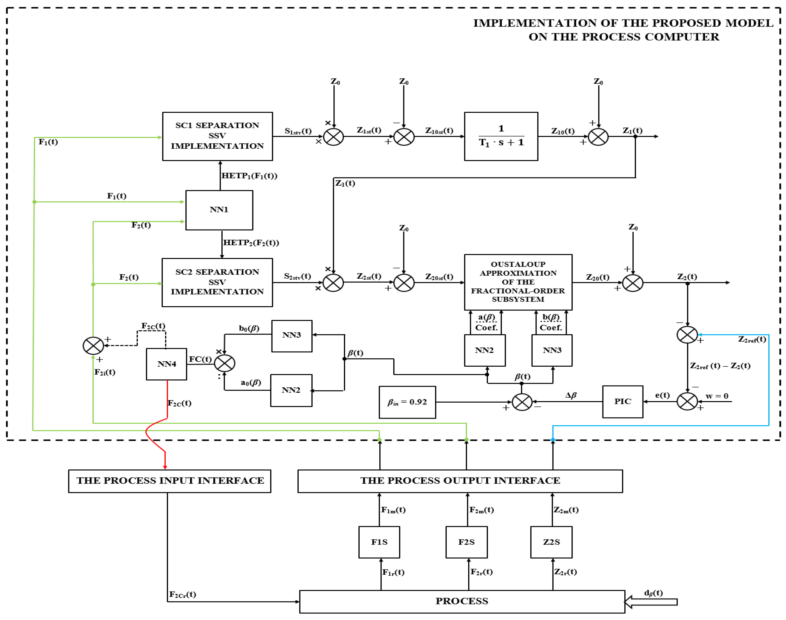
2.4. The Implementation of the Proposed Model

The implementation of the proposed mathematical model, which describes the separation cascade operation on the process computer from the architecture of the proposed monitoring system (described in the following sections of the manuscript), is based on the structure presented in Figure 6.

In the upper part of the structure, the mathematical model which describes the SC1 operation is implemented. The SC1 Separation SSV element implements the second factor of the right member of (1); it generates, based on the input signal F₁(t), the steady-state value of the separation associated with SC1 (S_1stv(t)). The multiplication element and the subtraction element are consecutively used for obtaining the Z_1st(t) and Z_10st(t) signals. After applying the Laplace transform to (8), the transfer function which connects the signals Z_10st(s) = L{Z_10st(t)} and Z₁₀(s) = L{Z₁₀(t)} is given by:

$${\mathrm{H}}_1\left(\mathrm{s}\right)=\frac{{\mathrm{Z}}_{10}\left(\mathrm{s}\right)}{{\mathrm{Z}}_{10\mathrm{s}\mathrm{t}}\left(\mathrm{s}\right)}=\frac{1}{{\mathrm{T}}_1·\mathrm{s}+1}$$

(12)

Finally, by using the last adder from the right part (of the upper structure), (9) is implemented, resulting the Z₁(t) signal, more exactly the output signal (the ¹⁸O isotope concentration) at the output (top) of SC1.

Using a similar procedure, the signals S_2stv(t), Z_2st(t) and Z_20st(t) are obtained for the case of SC2 (the input signal being F₂(t)). Additionally, in this case, the SC2 Separation SSV element implements the entire (1). The HETP₁(F₁(t)) and HETP₂(F₂(t)) functions are modeled using the neural network NN1, which, consequently, has two inputs and two outputs. The interconnection between the SC1 model and the SC2 model is made (using an arrow) by the fact that Z₁(t) is the input ¹⁸O isotope concentration in SC2 (SC2 separates the ¹⁸O isotope already separated by SC1).

In order to implement (10), the Oustaloup approximation of the 5th order is used. The main challenge in this context is represented by the fact that the differentiation order β associated with the fractional-order model of SC2 can present variations during the separation cascade operation (due to the parametric disturbances which occur in the separation plant operation). In this context, an original solution for modeling and simulating a fractional-order process with variable differentiation order is proposed. This solution is based on variating all the coefficients of the Oustaloup approximation at the variation of β. Considering initially β constant at the nominal identified value of 0.92, after applying the Laplace transform to (10), the transfer function which connects the signals Z_20st(s) = L{Z_20st(t)} and Z₂₀(s) = L{Z₂₀(t)} is given by:

$${\mathrm{H}}_2\left(\mathrm{s}\right)=\frac{{\mathrm{Z}}_{20}\left(\mathrm{s}\right)}{{\mathrm{Z}}_{20\mathrm{s}\mathrm{t}}\left(\mathrm{s}\right)}=\frac{{\mathrm{K}}_{\mathrm{I}}}{{\mathrm{T}}_2·{\mathrm{s}}^{\beta }+1}$$

(13)

The general form of the 5th order Oustaloup approximation for the fractional order transfer function from (13), considering, also, the β differentiation order variation (β = β(t)), has the following form:

$${\mathrm{H}}_{2\mathrm{O}\mathrm{u}\mathrm{s}\mathrm{t}}\left(\mathrm{s}\right)={\mathrm{K}}_{\mathrm{I}}\left(\beta \right)·\sum _{\mathrm{i}=5}^0\frac{{\mathrm{a}}_{\mathrm{i}}\left(\beta \right)·{\mathrm{s}}^{\mathrm{i}}}{{\mathrm{b}}_{\mathrm{i}}\left(\beta \right)·{\mathrm{s}}^{\mathrm{i}}}$$

(14)

where ${\mathrm{a}}_{\mathrm{i}}\left(\beta \right)$ and ${\mathrm{b}}_{\mathrm{i}}\left(\beta \right)$ (i$\in$ {0; 1; 2; 3; 4; 5}) are the coefficients of the numerator, respectively, of the denominator of the H_2Oust(s) transfer function and K_I($\beta$) is the proportionality constant necessary for the compensation of the output signal steady state value (due to the usage of the fractional-order model for modeling the behavior of the separation process associated to SC2) in order to preserve the imposed concentration steady state value of the produced ¹⁸O isotope. It can be remarked that ${\mathrm{a}}_{\mathrm{i}}\left(\beta \right)$, ${\mathrm{b}}_{\mathrm{i}}\left(\beta \right)$ and K_I($\beta$) are functions depending on the β differentiation order.

The neural networks NN2 and NN3 have both as input signal the $\beta \left(t\right)$ function (the variation of the differentiation order in relation to time) and generate at the outputs the ${\mathrm{a}}_{\mathrm{i}}\left(\beta \right)$ coefficients (NN2), respectively, ${\mathrm{b}}_{\mathrm{i}}\left(\beta \right)$ coefficients (NN3). The element “Oustaloup Approximation of the Fractional-Order Subsystem” from Figure 6 implements under the integral form the Equation (14) considering, also, its variable coefficients generated by NN2 and NN3. Considering the final value theorem in the case of the step response of the transfer function from (14), it results in that:

$${\mathrm{Z}}_{20\mathrm{s}\mathrm{t}\mathrm{v}}\left(\mathrm{t}\to \mathrm{\infty }\right)=\underset{\mathrm{s}\to 0}{\lim }{\mathrm{H}}_{2\mathrm{O}\mathrm{u}\mathrm{s}\mathrm{t}}\left(\mathrm{s}\right)=\frac{{\mathrm{a}}_0\left(\beta \right(\mathrm{t}\left)\right)}{{\mathrm{b}}_0\left(\beta \right(\mathrm{t}\left)\right)}$$

(15)

where Z_20stv is the ¹⁸O isotope concentration increase over Z₀ at the output of the separation cascade. (15) shows the necessity of using a compensation procedure in order to obtain the imposed ¹⁸O isotope at the separation cascade output when $\beta$ parameter presents variations in relation to time. This aspect is due to the fact that in practice Z_20stv $\ne$ 1 (a₀(β(t) $\ne$ b₀(β(t)). In this context, the necessary compensation is given by:

$${\mathrm{K}}_{\mathrm{I}}\left(\beta \right(\mathrm{t}\left)\right)=\frac{b_0\left(\beta \right(\mathrm{t}\left)\right)}{{\mathrm{a}}_0\left(\beta \right(\mathrm{t}\left)\right)}$$

(16)

and the previously introduced notation (in the case of (10)) is K_I = K_I(0.92). (16) highlights the solution to compute the compensation constant K_I(β(t)), the a₀(β(t)) and b₀(β(t)) coefficients being already available at the outputs of NN2 and NN3 as it is shown in Figure 6. However, the compensation constant K_I(β(t)) can be used only in the case of the mathematical model simulation. In the real case, the compensation is made through the appropriate adjustment of the F₂(t) nitric oxide input flow. The mentioned appropriate value is also generated based on the proposed model. In this context, the FC(t) signal (flow compensation signal) has a value equal to that of K_I(β(t)), and it represents the input signal in NN4. The NN4 neural network implements the following non-linear equation:

$${\mathrm{F}}_{2\mathrm{C}}\left(\mathrm{t}\right)=\mathrm{s}\mathrm{i}\mathrm{g}\mathrm{n}\left[{\mathrm{Z}}_{\mathrm{s}\mathrm{t}\mathrm{i}\mathrm{m}\mathrm{p}}\left(1-\frac{1}{\mathrm{F}\mathrm{C}\left(\mathrm{t}\right)}\right)\right]·{\mathrm{H}\mathrm{E}\mathrm{T}\mathrm{P}}_2^{-1}\left(\frac{\mathrm{h}·\mathrm{C}}{\mathrm{C}·\left[{\mathrm{l}\mathrm{o}\mathrm{g}}_{\mathsf{\alpha }}\left(\frac{\left|{\mathrm{Z}}_{\mathrm{s}\mathrm{t}\mathrm{i}\mathrm{m}\mathrm{p}}(1-\frac{1}{\mathrm{F}\mathrm{C}\left(\mathrm{t}\right)})\right|}{{\mathrm{Z}}_0}\right)\right]-\mathrm{h}}\right)$$

(17)

It generates correction flow at the F_2C(t). Figure 6 shows that the model allows the compensation through the F₂(t) (F₂(t) = F_2i(t) + F_2C(t), where F_2i(t) is the non-compensated nitric oxides input flow in SC2, but in this case, it is not necessary to use the K_I(β(t)). However, in the case of the proposed mathematical model, the usage of K_I(β(t)) is preferred (for this reason, the F_2C(t) signal is symbolized with a discontinuous arrow in Figure 6, case when F₂(t) = F_2i(t)). The compensation flow F_2C(t) is transmitted to the real process through the “Process Input Interface”.

Using the flow sensors F1S and F2S, respectively, the concentration sensor Z2S, the real values F_1r(t), F_2r(t) and Z_2r(t) of the F₁(t), F₂(t) and Z₂(t) signals are measured, they generate at their outputs the measured values F_1m(t), F_2m(t) and Z_2m(t). The values of the F_1m(t), F_2m(t) and Z_2m(t) signals are transmitted to the proposed mathematical model in order to be processed through the “Process Output Interface”. By making the difference Z_2ref(t) − Z₂(t) (where the reference value Z_2ref(t) = Z_2m(t), the deviation of the output signal generated the proposed model in relation to the real value of the ¹⁸O concentration at the separation cascade output results (this deviation is due to the d_β(t) disturbance signal which affects the separation process directly as it is highlighted in Figure 6; d_β(t) disturbance signal implies the direct variation of the β differentiation order). By imposing this deviation at the value w = 0, the error signal e(t) = Z₂(t) − Z_2ref(t) can be computed. Using a Proportional integral Controller (PIC), which processes the error signal e(t), the Δβ(t) adjustment signal is generated at its output. This signal is used to adjust the value of β(t) differentiation order based on the equation: β(t) = β_in − Δβ(t), where β_in = 0.92 is the initial identified value of β. Consequently, the proposed mathematical model identifies in online mode the new β differentiation order implied by the disturbance action, and it adapts online its coefficients accordingly. Implicitly, through NN4, it generates the necessary compensation in order to reject the effect of the mentioned type of disturbance.

In addition to the model whose structure is presented in Figure 6, another neural network (NN5) is used to implement (5) and to generate the appropriate value of F₂(t) in order to obtain the imposed ¹⁸O isotope concentration, in a steady-state regime, at the separation cascade output in normal operation regime (without the disturbances occurring in the process).

The details regarding the neural networks used in implementing the proposed mathematical model are centralized in

Table 2. They used neural networks.

Neural Network	Input Signal/Signals	Output Signal/Signals	Number of Hidden Layers	Size of Hidden Layer/Layers	Size of Output Layer
NN1	F1(t) F2(t)	HETP1(F1(t)) HETP2(F2(t))	1	18	2
NN2	β(t)	${\mathrm{a}}_{\mathrm{i}}\left(\beta \right)$ (i$\in$ {0; 1; 2; 3; 4; 5})	2	[23; 10]	6
NN3	β(t)	${\mathrm{b}}_{\mathrm{i}}\left(\beta \right)$ (i$\in$ {0; 1; 2; 3; 4; 5})	2	[25; 14]	6
NN4	FC(t)	F2C(t)	1	14	1
NN5	Zstimp(t)	F2(t)	1	17	1
Neural Network	Activation Functions of the Neurons from the Hidden Layer/Layers	Activation Functions of the Neurons from the Output Layer	Maximum Training Epochs	Run Training Epochs	Learning Algorithm
NN1	Bipolar sigmoid	Linear	50,000	43,243	Levenberg–Marquardt
NN2	Bipolar sigmoid	Linear	75,000	58,234	Levenberg–Marquardt
NN3	Bipolar sigmoid	Linear	80,000	73,692	Levenberg–Marquardt
NN4	Bipolar sigmoid	Linear	30,000	18,217	Levenberg–Marquardt
NN5	Bipolar sigmoid	Linear	32,000	25,875	Levenberg–Marquardt

.

In all cases, after training, the correlation coefficients between the experimental responses and the responses resulting after the solution’s neural networks simulation are higher than 98.8%. The implementation of the neural networks from Figure 6 is made by implementing their corresponding equations and considering the solution weights and bias values resulting after the training algorithm. As an example, the equation which describes the NN2 operation is given:

$$\mathrm{A}\left(\mathrm{t}\right)={\mathrm{W}}_{23}·\mathrm{b}\mathrm{s}\left({\mathrm{W}}_{12}·\mathrm{b}\mathrm{s}\left({\mathrm{W}}_{01}·\beta \left(\mathrm{t}\right)+{\mathrm{B}}_1\right)+{\mathrm{B}}_2\right)+{\mathrm{B}}_3$$

(18)

where A(t)[6 × 1] is the output vector which contains the ${\mathrm{a}}_{\mathrm{i}}\left(\beta \right)$ (i$\in$ {0; 1; 2; 3; 4; 5}) coefficients, $\beta \left(\mathrm{t}\right)$[1 × 1] is the input signal, W₀₁[23 × 1] is the solution vector having as elements the weights which connect the input layer (containing the input signal) with the first hidden layer, B₁[23 × 1] is the solution vector which contains the bias values of the neurons from the first hidden layer, W₁₂[10 × 23] is the solution matrix having as elements the weights which connect the first hidden layer with the second hidden layer, B₂[10 × 1] is the solution vector which contains the bias values of the neurons from the second hidden layer; W₂₃[6 × 10] is the solution matrix having as elements the weights which connect the second hidden layer with the output layer, B₃[6 × 1] is the solution vector which contains the bias values of the neurons from the output layer, respectively, the notation bs() signifies the application of the non-linear sigmoid bipolar function.

The usage of neural networks implies some major advantages: high accuracy; generality based on the universal approximation property; high validity due to the fact that the solutions result after a learning algorithm application; the possibility to process a large amount of data and to model more than one functional dependency simultaneously, due to their parallel structure.

The neural networks, which contain in their structure two hidden layers, generate at their outputs the values of the coefficients of the 5th-order Oustaloup approximation for the determined fractional-order transfer function (NN2 generates the values of the numerator coefficients, and NN3 generates the values of the denominator coefficients). The increase of the training precision of the NN2 and NN3 is necessary for two reasons:

• they have multiple output signals (each of the two neural networks generates six output signals), an aspect which increases the complexity of the functional dependency between the input signal (the fractional differentiation order) and the output signals;
• in each neural network case, the values of the six output signals present consistent variations from one signal to another one; more exactly, some coefficients have significantly high values and other coefficients have much more small values; in this context, the error obtained after training the two neural networks has to be consistently smaller (of at least 1000 times, for a good accuracy) than the value of the smallest generated coefficient, an aspect which is difficult to be obtained due to the higher values of the other coefficients.

Consequently, in order to obtain better accuracy, the computation capacities of the NN2 and NN3 neural networks were increased by introducing, in both cases, the second hidden layer. Additionally, the number of neurons in the first hidden layer was increased (in both cases) by comparison with the other used neural networks. By applying these procedures, the imposed target errors were obtained, and the correctness of using NN2 and NN3 was ensured. Using the proposed structures of NN2 and NN3, their modeling accuracy was increased significantly than in the case of using only one hidden layer (practically, using only one hidden layer, the target errors, in both cases, were not reached).

Synthesizing, the stages of identifying the proposed mathematical model, are:

• Analyzing experimental data and displaying them graphically.
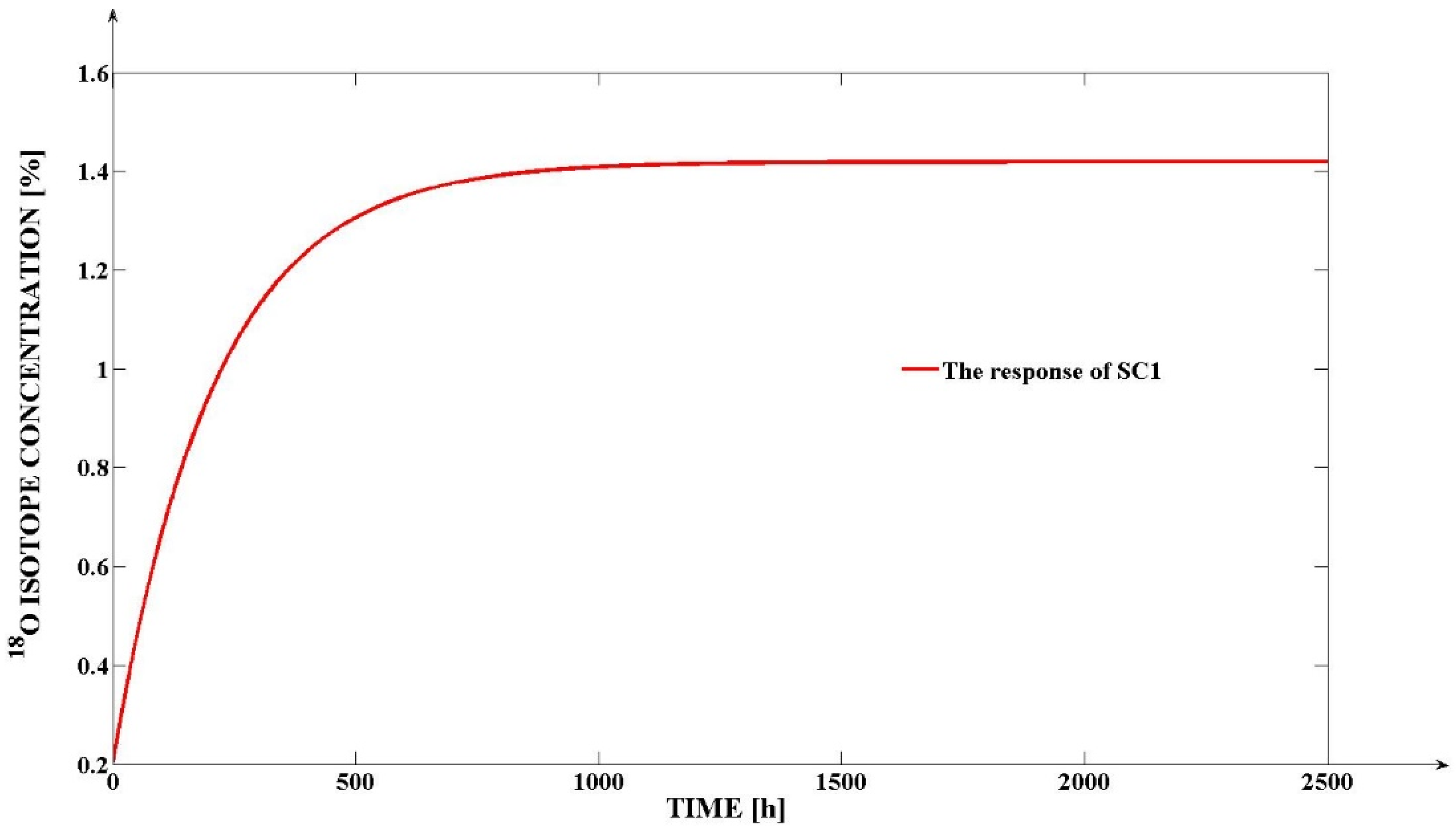
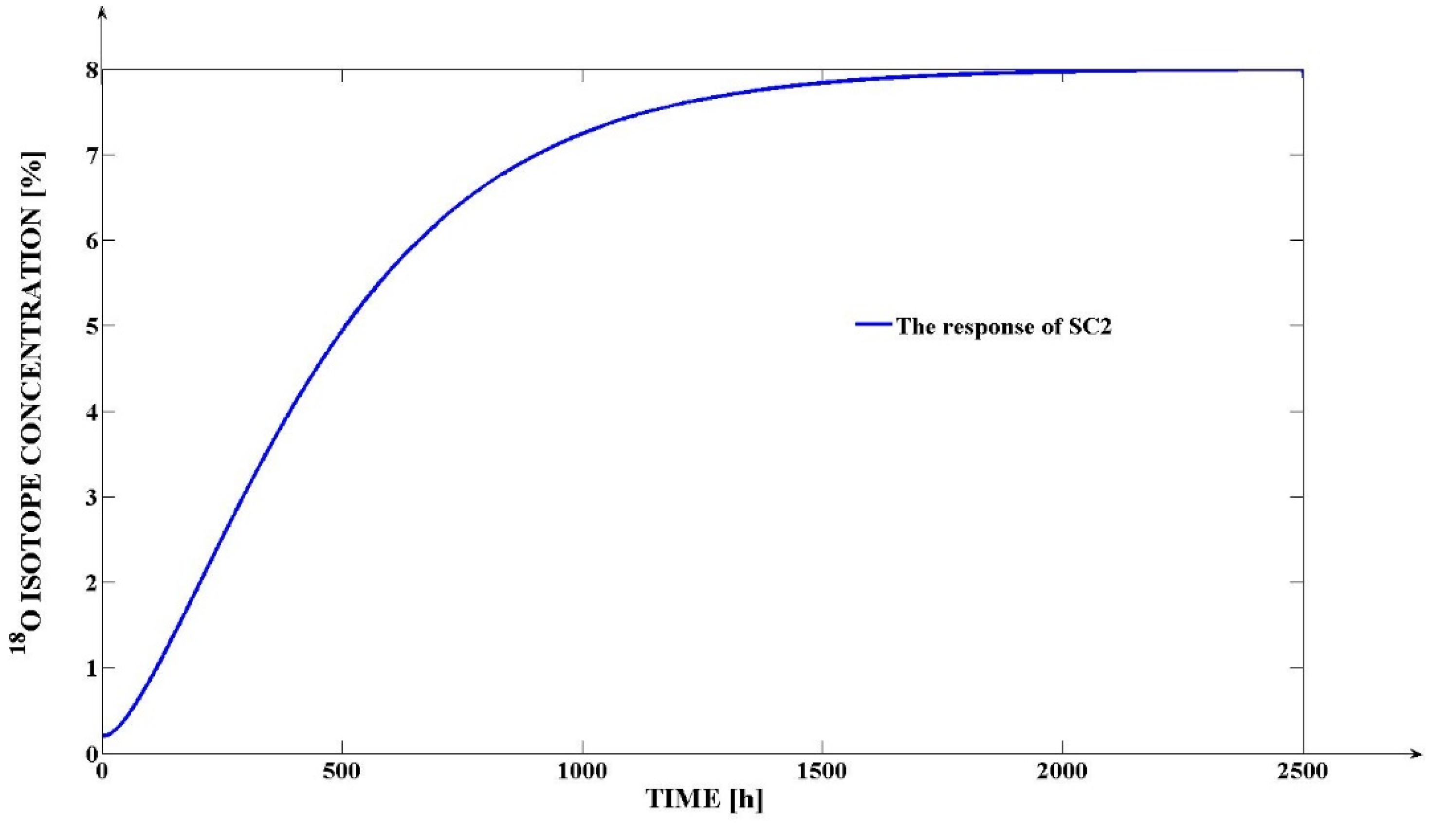
• The analytical determination of the steady-state values of the ¹⁸O isotope concentrations at the top of the two separation columns (these steady-state values are obtained based on the separations functions, which are nonlinear functions depending on other nonlinear functions (more exactly, on the heights of equivalent theoretical plates)).
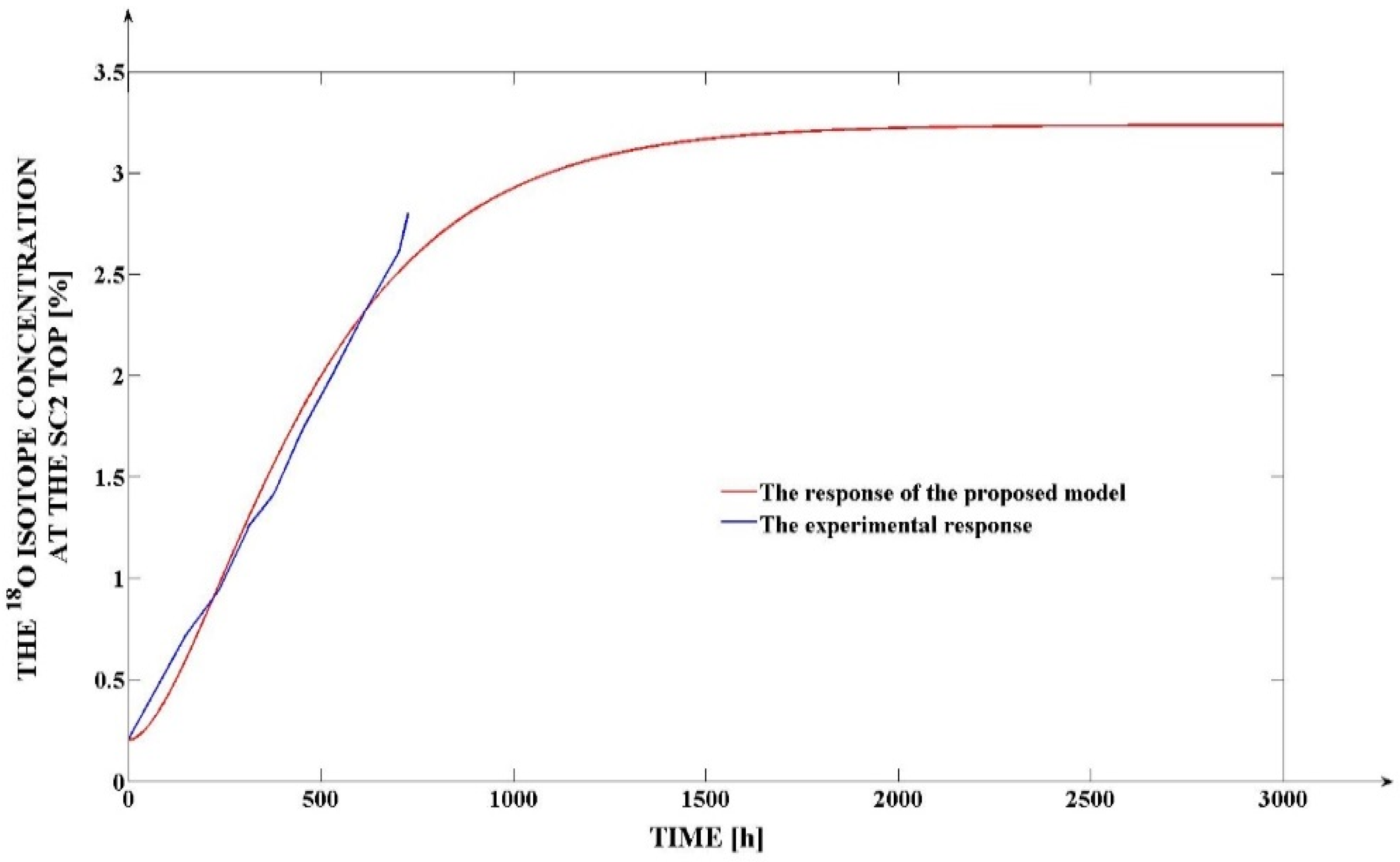
• The determination of the system of Equations (8)–(11), which describes the separation cascade behavior in a dynamical regime. As results from (10), the proposed mathematical model is a fractional-order one.
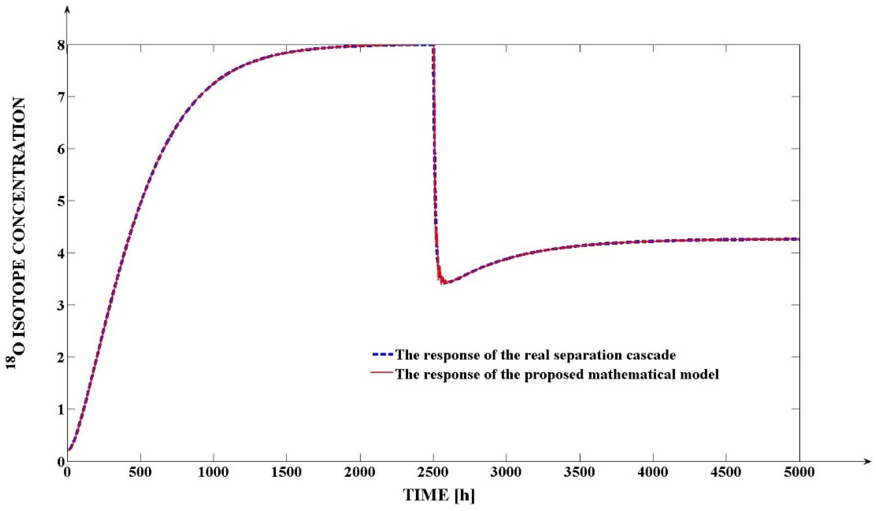
• The application of the proposed iterative procedure used for obtaining the proposed mathematical model’s structure parameters (the set of (T₁, T₂ and β) parameter values which generate the best fit between the experimental response and the response generated by the proposed mathematical model).
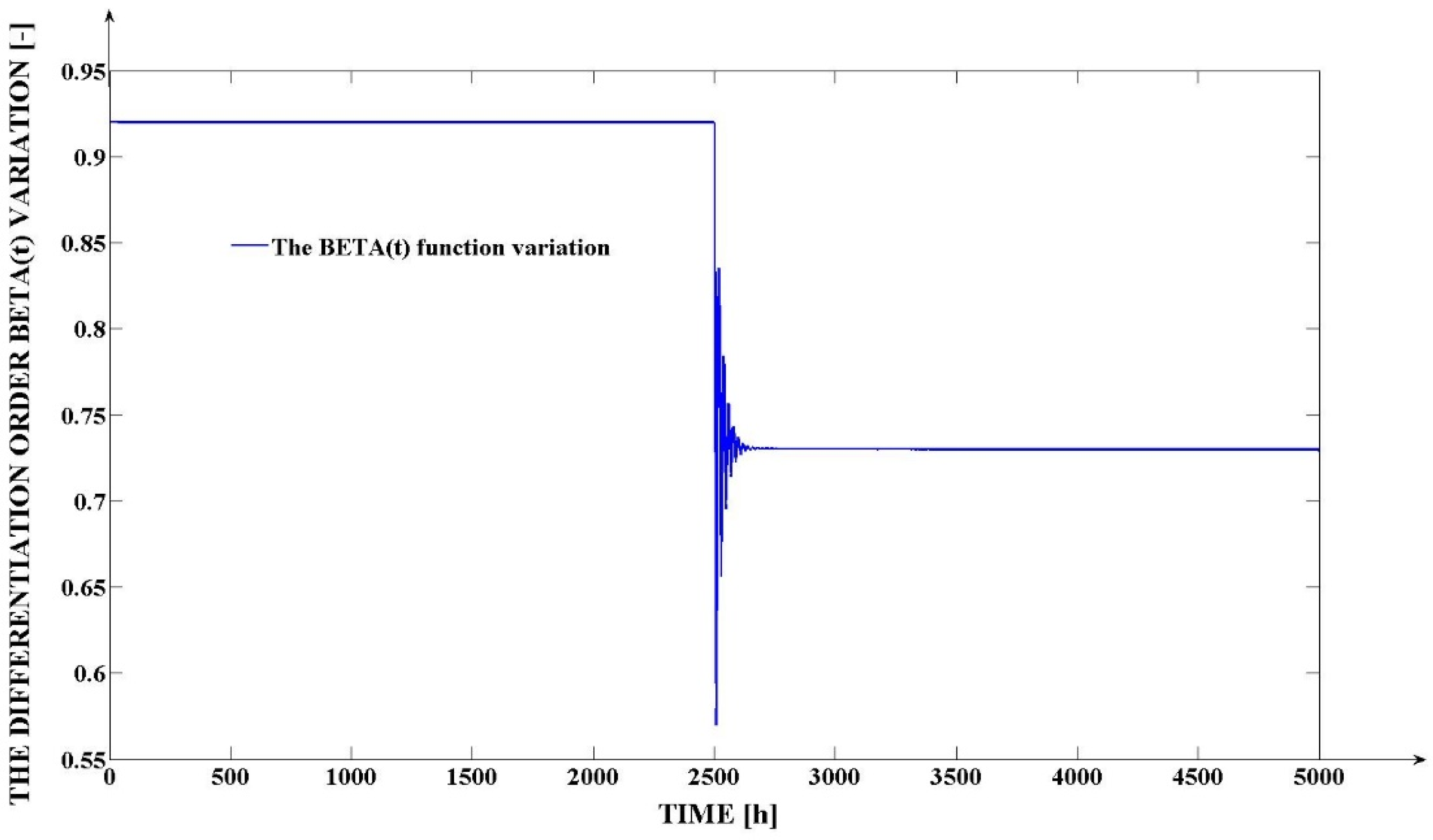
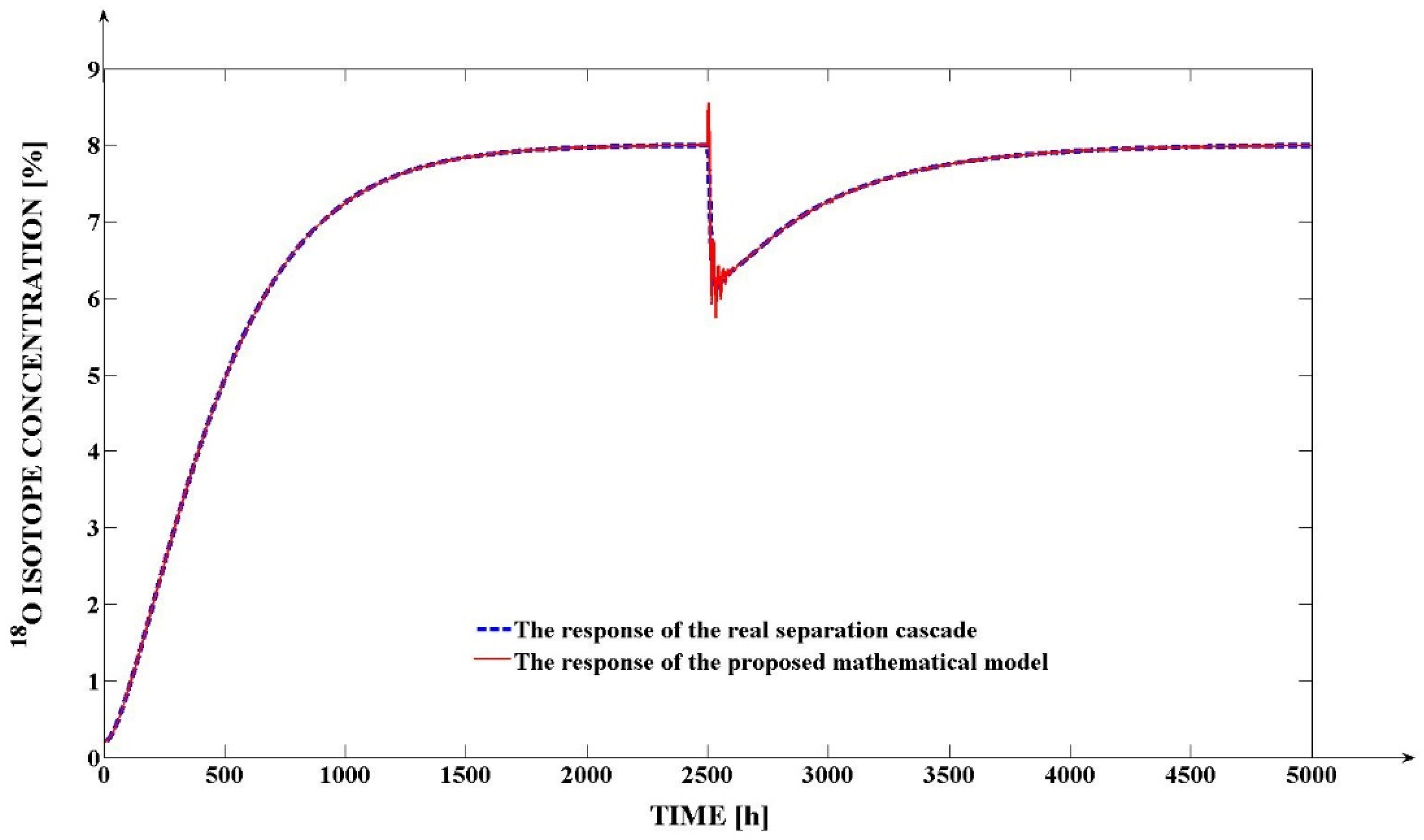
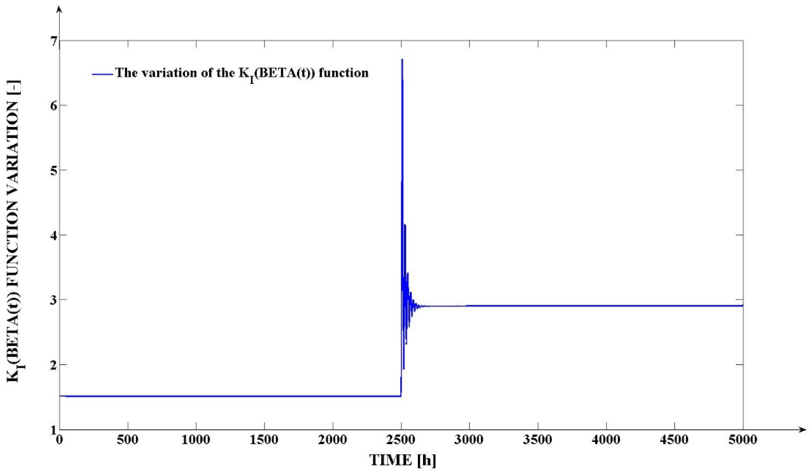
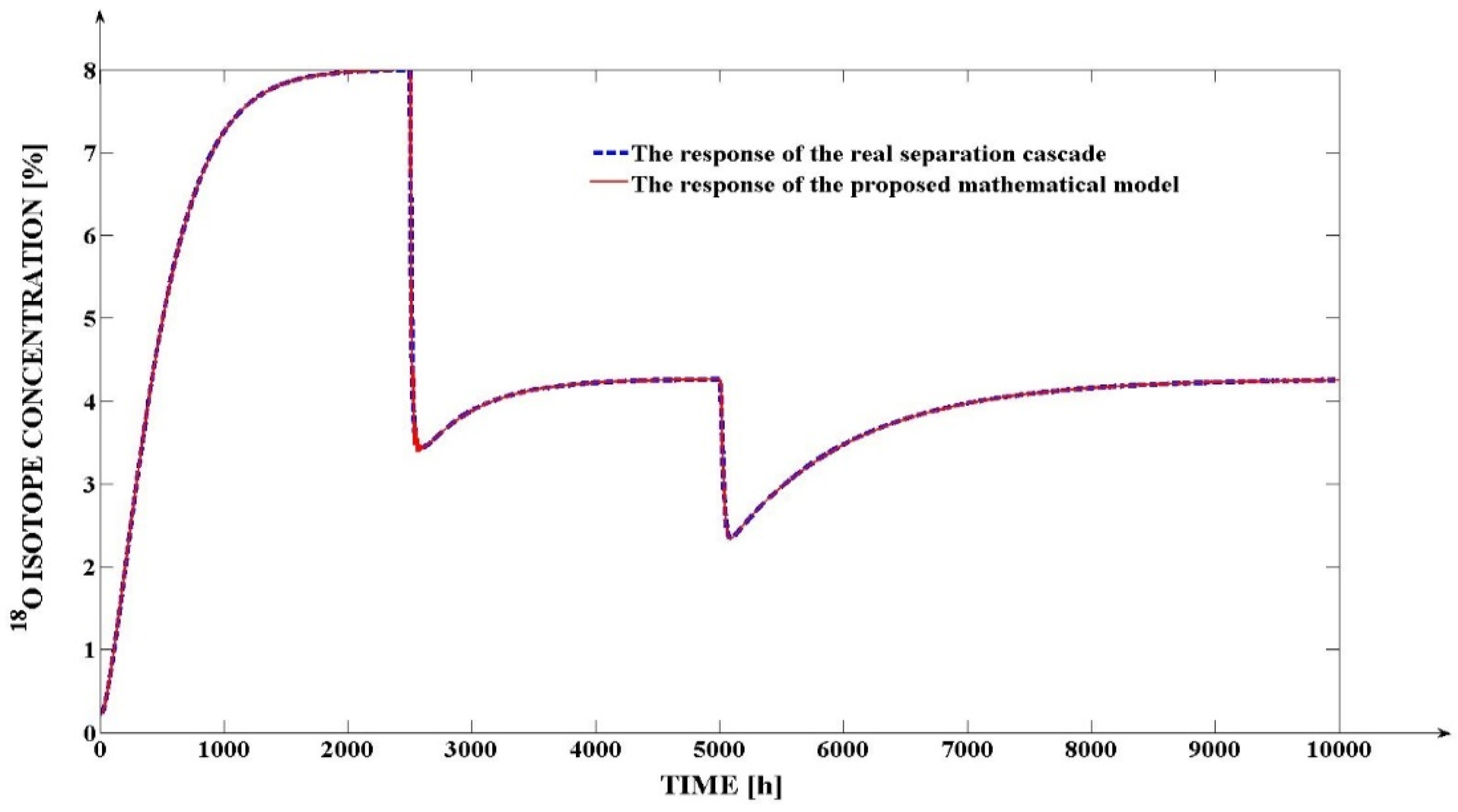
• The determination of the original solution applicable for the simulation of the proposed mathematical model in the context when the main considered parametric disturbance is the variation of the fractional differentiation order (β) of the fractional component of the model.
• The training of the neural networks is used for the implementation of the separation process nonlinearities and its fractional-order component.
• The implementation of the proposed mathematical model functional diagram.

3. Method of Implementing Remote Process Monitoring

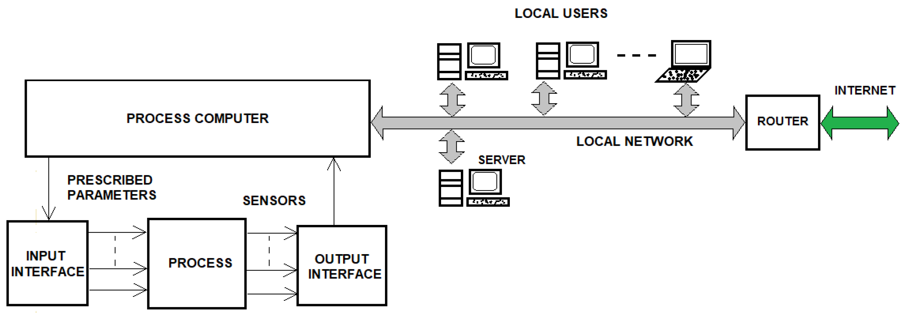
3.1. Preliminaries Regarding the Informatic System for a Technological Process Control

Figure 7 shows the block diagram of a computer system for the automatic control of a technological process. The process computer is in charge of the complete technological process, and the entrance-exit interface is used to adjust the parameters’ values. A local operator may have access to details about the operation’s status, real-time parameters, and planned parameters through terminals connected to the local network (pressure, temperature, and concentration of interest isotopes) [8].

The block diagram of the automatic control computer system will be changed to allow remote monitoring of this process, as shown in Figure 8, where the dotted part was added to Figure 7.

During the process, the monitoring interface takes control or provides remote operators with the relevant parameters.

Despite the interface being identical to a process computer’s, different parameters may be of importance for remote monitoring.

A computer for process monitoring has also been introduced. This computer is home to a database containing the names of the process supervisors and an application that communicates with the monitoring interface.

Only operators who have registered in this database have access to process information, and their privileges are hierarchical. Operators are registered in a database on the monitoring computer to prevent unsuccessful process interventions.

Operators who have enrolled in this database can receive information on the state of the process, as well as numerical or logical values for process parameters, by SMS or E-Mail on a smart device, tablet, smartphone, desktop computer, or laptop.

Local operators can complete these tasks using their local network, but for those who are located further away, remote communication networks are required (via the internet or fixed or mobile phone network).

After a brief review of the most popular types of interfaces and communicators, taking into account the possibility of connecting as efficiently as possible to the existing sensors of the process, we decided that the RS485 interface is more suitable for remote parameter monitoring and transmission interface.

The RS485 interface is very versatile, easy to implement, has good immunity to disturbances, can connect several devices (ModBus mode) and can communicate over long distances (maximum 1200 m).

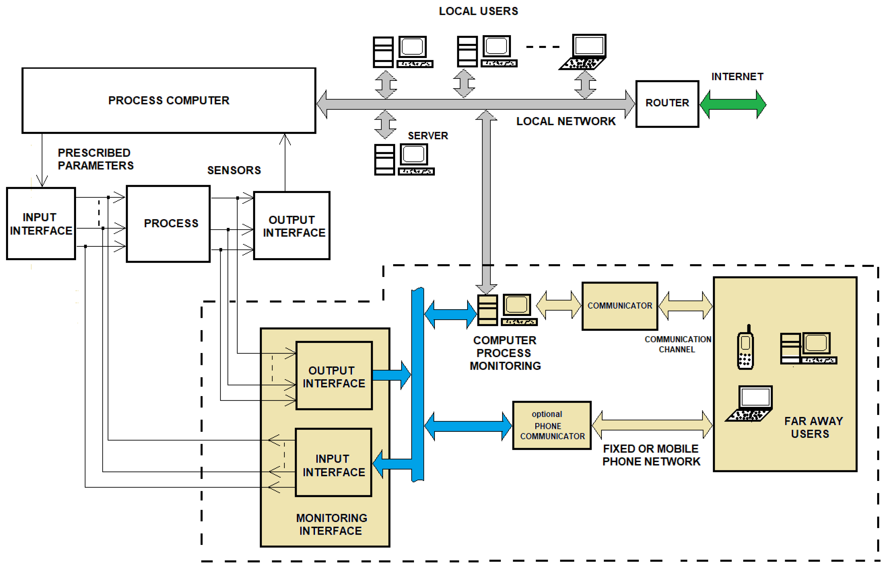
3.2. Remote Monitoring Interface of the ¹⁸O Isotope Production Process by NO-HNO₃ (H₂O) Isotopic Exchange Reaction

Figure 9 shows the complete principal diagram of the monitoring interface. This interface is designed to monitor six logical parameters (ON/OFF values) and six numerical parameters (temperatures). They will be noted as follows:

H2—the presence of H2 gas pressure of at least 4 bars

AE1—electric arc operation in cracking reactor 1

AE2—electric arc operation in cracking reactor 2

AE3—electric arc operation in cracking reactor 3

AE4—electric arc operation in cracking reactor 4

AE5—electric arc operation in the cracking reactor at column 2

TCP1—Preheating oven temperature at column 1

TRCC1—Catalytic conversion reactor temperature at column 1

TRCA1—Ammonia cracking reactor temperature at column 1

TCP2—Preheating oven temperature at column 2

TRCC2—Catalytic conversion reactor temperature at column 2

TRCA2—Column 2 ammonia cracking reactor temperature

The system monitoring interface uses an RS485 interface to read the six temperatures by the microcontroller A (Master) through a ModBus protocol.

Microcontroller A runs a program that reads the digital inputs D1, D2, D3, D4, D5, and D6, respectively, the signal for gas pressure H2 and the five signals for currents in the five crack reactors. From sensors to microcontrollers, the communication protocol in this stage is unidirectional PTP. Only MAX485 circuit pairs are employed to deliver logic signals to microcontroller A’s inputs D1, D2, D3, D4, D5, and D6.

To monitor the H₂ gas pressure, the signal from the monostable circuit output is sent to the microcontroller via MAX485-type integrated circuits used in RS485-type interfaces.

Closing the electrical circuit of the contacts on the manometer will reveal the presence of a “logic 0” level at the input of the monostable CBM circuit and at its output Q when the H2 gas pressure falls below 4 bars.

The ZMCT103 type mini-current transformer has a 10:1000 transformation ratio and detects the existence of electric current in the circuit, which should be around 2 A under typical working conditions.

The secondary current provided by the current transformer is proportional to the primary current measured (for the ratio 10:1000, at 5 A in the primary, 50 mA at the output). Through the R_o resistor, this current is transformed from current to voltage, rectified by a PR rectifier bridge, and filtered by a 470 μF capacitor.

A U_o voltage is obtained at the terminals of the resistor R_o, corresponding to the current I_o from the current transformer’s output.

In this situation, we have for I_o = 2 mA:

U_o = R_o ∗ I_o = 200 ∗ I_o = 200 ∗ 0.02 A = 4 V

(19)

This voltage is used to control the “+” input of an LM339 comparator integrated circuit.

A voltage of roughly +5 V (logic level 1) will be obtained at its output.

When there is no electric current in the primary circuit, the current I_o = 0 A produces U_o = 0 V, and the voltage at the comparator C’s output is approximately 0 V (logic level 0). The voltage from the C comparator output is applied to the MAX485 circuit’s DI input for further transmission.

The monitoring interface’s output is read on a digital input D2 of the microcontroller A and transferred to the process monitoring computer through a USB port. On the microcontroller’s inputs D3, D4, D5, and D6, the same is read for the other three crack reactors. Because the distances between the measurement points and the monitoring interface can be wide, and this interface can communicate up to 1200 m, we picked an RS485 bus type for temperature monitoring in six points.

Another alternative was to use an integrated temperature sensor module with an RS485 interface and attach it to microcontroller A directly via the RS485 bus. The microcontroller 1–6, which is close to the thermocouple corresponding to Th 1–6, “reads” and stores the values provided by the specialized circuit MAX6685 and the thermocouples Th1, Th2, … Th6 through the SPI interface.

A separate display of the read temperature can also be built with three or four numbers. Microcontroller A (Master) interrogates, in turn, microcontrollers 1–6, which will read the values of the temperatures provided by the Th1-Th6 thermocouples and communicate them via a USB port to the monitoring computer via the RS485 ModBus protocol interface. All of the data collected by microcontroller A is transferred to the monitoring computer via USB.

The process monitoring computer runs software that reads these values, maintains a database with users and their privileges, and sends notification e-mails or SMS to operators based on the primate values of the parameters.

Six numerical parameters in the process (temperatures measured with Pt-PtRh thermocouple sensors) and six logic parameters (operation of the electric arc in the five crack reactors of the system, respectively, the presence of a pressure of at least bar when supplying H2 to the installation) are monitored by means of this interface. As mentioned previously, temperature monitoring in all the equipment operations from the separation cascade is very important in order to maintain the elementary separation factor of the ¹⁸O isotope (α) constant and to analyze its possible deviations near the value of 1.018.

4. Results

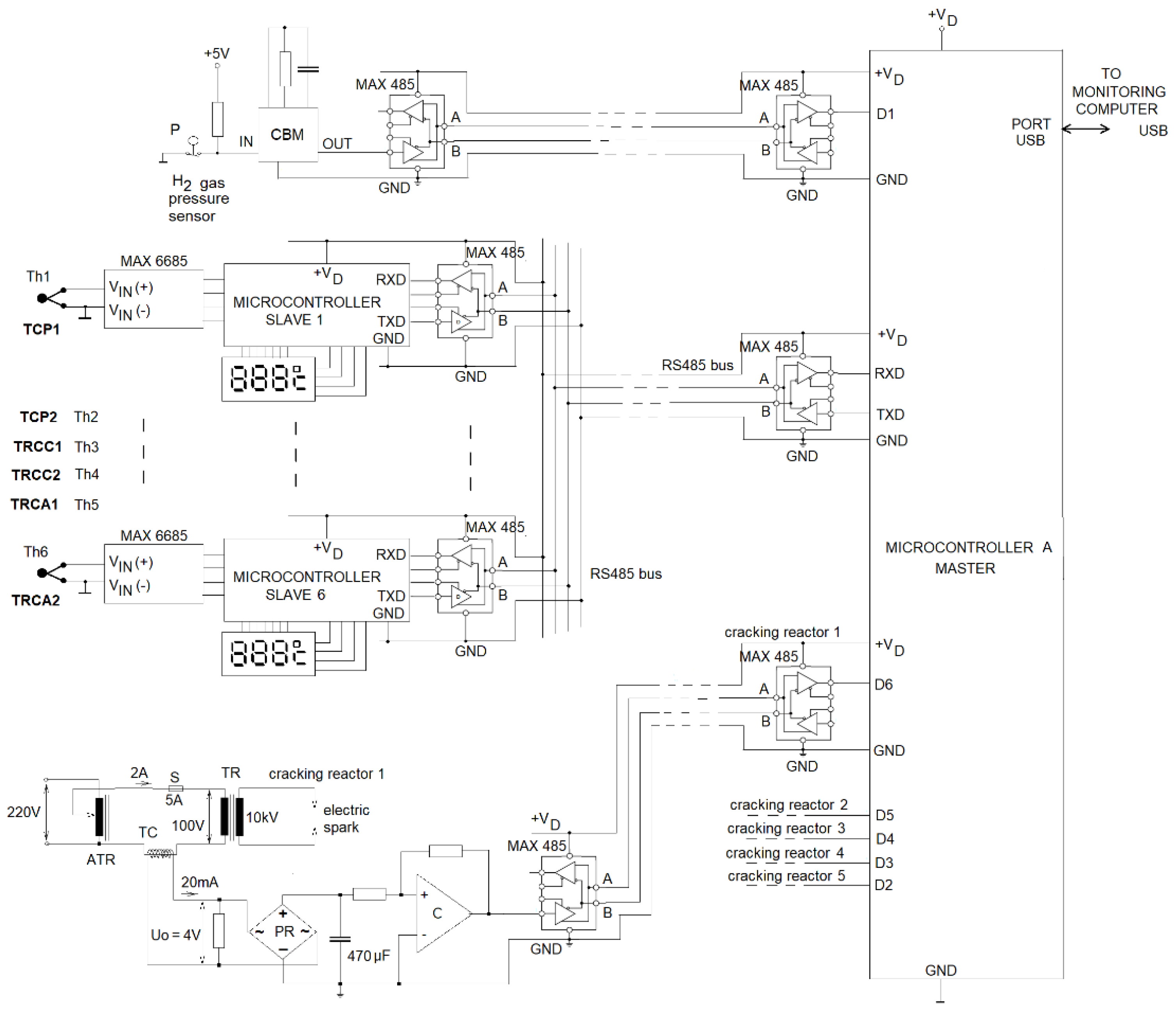
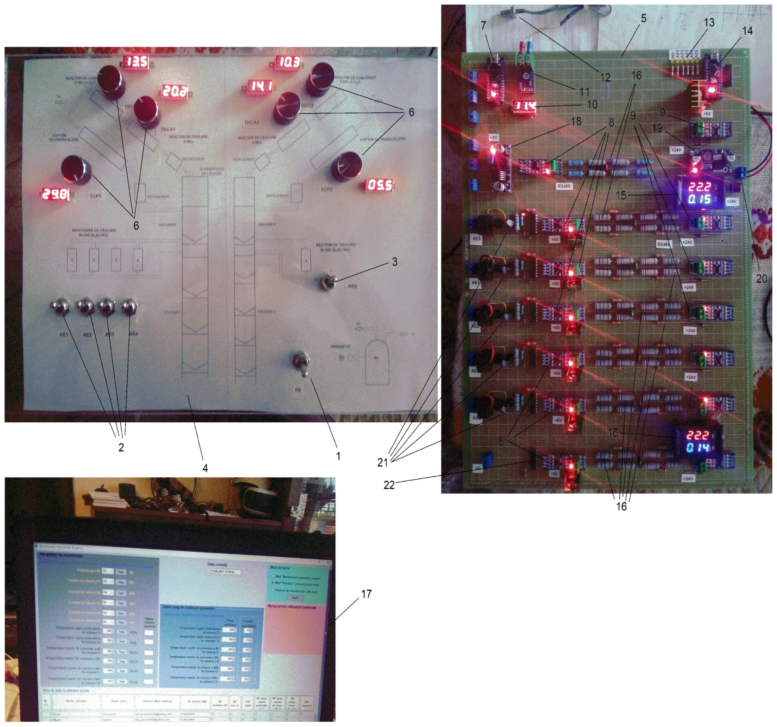
4.1. Interface Board

Based on the principal scheme above, an experimental board was built, which is presented in Figure 7. An attempt was made to reproduce the field conditions as closely as possible by simulating the length of the communication network cables and testing the feeding of the end devices through these cables.

This board is connected to a simulation panel, from which the monitored sensors can be simulated, or via the USB port of the microcontroller to a computer running the monitoring software.

The inputs of the logical parameters—the existence of 4 bar H₂ pressure and the existence of an electric arc in the cracking reactors—were simulated with switch six and switches 1–5, respectively.

In order to ensure better management of the temperature values in the simulations, five of the temperature sensors were simulated using 50 KΩ linear potentiometers, along with a 3-digit display indicating the temperature the potentiometer is simulating (see Figure 9).

The current consumption in the cracking reactors was simulated with the help of the scheme in Figure 10.

In Figure 10 K2, K3, K4, K5, K6 are switches, TC1, TC2, TC3, TC4, TC5 are current transformers and R is a power consumer. The consumer R connected to the grid has a current consumption I:

I = P/U = 500/220 = 2.27 A

The switch K may or may not short-circuit the current transformer TC, i.e., it will or will not block the current flow through it. This allows simulation of the operation or interruption of the arc circuit in each cracking reactor individually.

Figure 11 shows a photo of the experimental system.

1—switch for simulating the existence of 4 bar H₂ pressure.

2,3—switch for simulating the operation or not of the electric arc.

4—panel.

5—experimental interface board.

6—potentiometers for simulating temperature variation.

7—microcontroller for temperature reading (Slave).

8,9—RS485 interface modules.

10—numerical temperature display from microcontroller for temperature reading.

11—MAX6675 circuit board.

12—K-type thermocouple temperature sensor.

13—control led for signals from sensors with logic values reaching microcontroller A.

14—microcontroller A (Master).

15—digital voltmeter–amperemeter for experimental consumption measurement.

16—long grid line simulator circuits (500 m).

17—monitoring computer.

18,19—5 V/2 A switching voltage stabilizer.

20—20 V interface board power supply.

21—arc monitoring circuits.

22—H₂ gas pressure monitoring circuit.

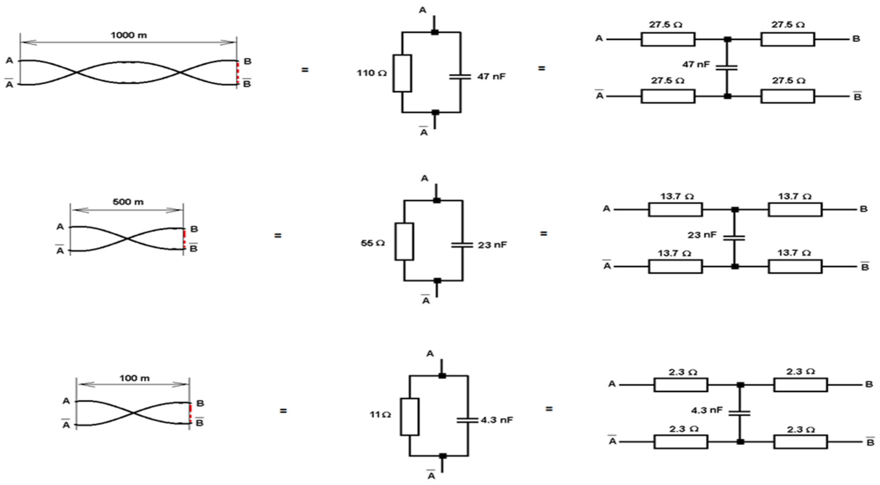
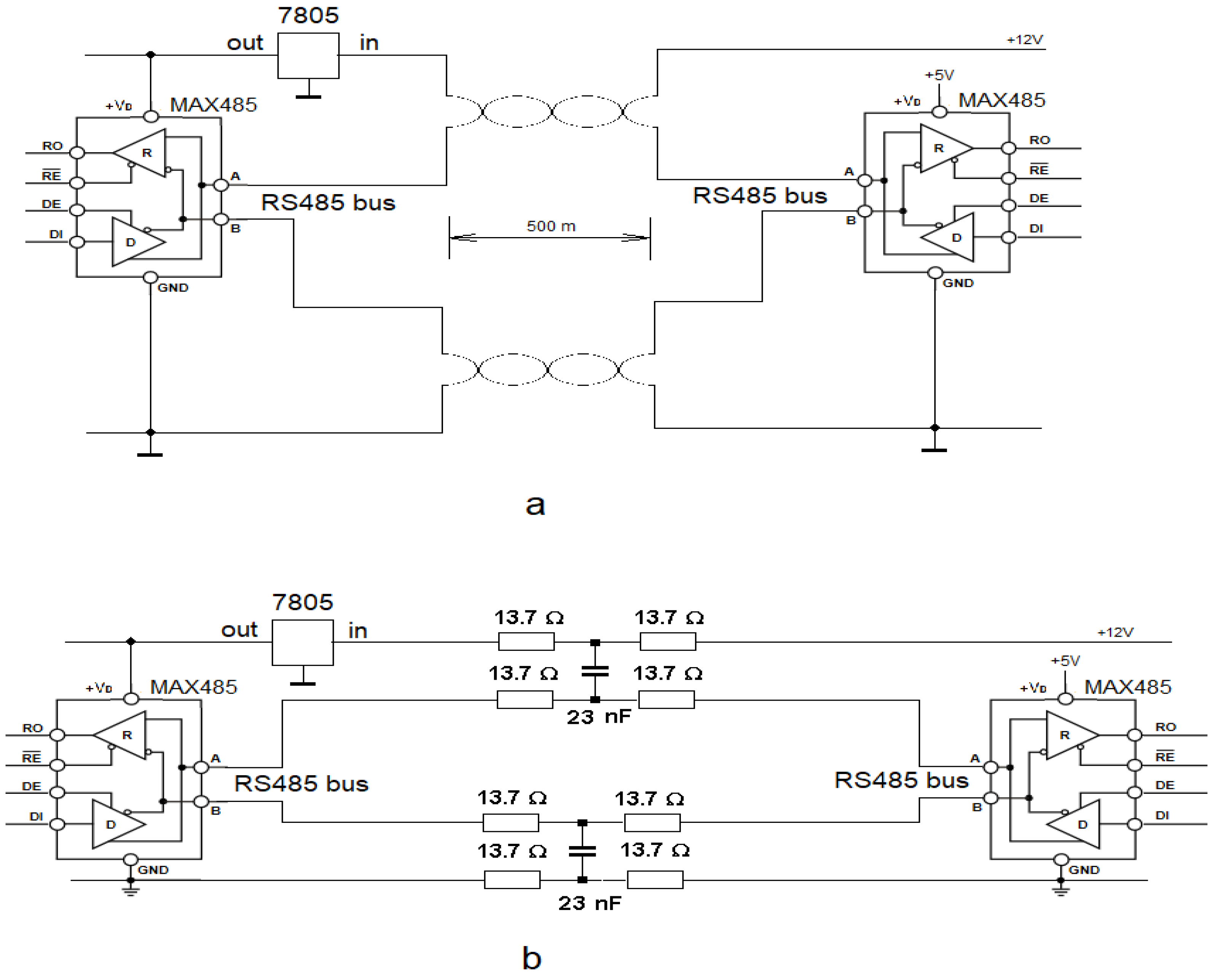
4.2. Simulation of Long Network Buses

Taking into account the characteristics of CAT.5 UTP twisted pair cable: loop electrical resistance: R < 188 Ω/1000 m and the specific electrical capacitance: C = 52 pF/m, the network equipment manufacturers recommend tests to simulate long looped power lines from UTP network cables, as presented in Figure 12.

Pairs A, $\stackrel{\_}{\mathrm{A}}$ and B, $\stackrel{\_}{\mathrm{B}}$ are the terminal points of each wire.

In order to simulate a 500 m long RS485 network with two pairs of twisted CAT.5 UTP cable, a circuit as in Figure 13 was used, with four groups of 13.7 Ω to 3 Ω resistors and a 23 nF capacitor.

The MAX485 circuit at the network end is fed from its counterpart at the other end of the network via one wire from the two pairs of twisted wires, as shown in Figure 13a. In order to simulate a 500 m long RS485 network with two pairs of twisted CAT.5 UTP cable, a circuit as in Figure 13b was used, with four groups of 13.7 Ω to 3 Ω resistors and a 23 nF capacitor.

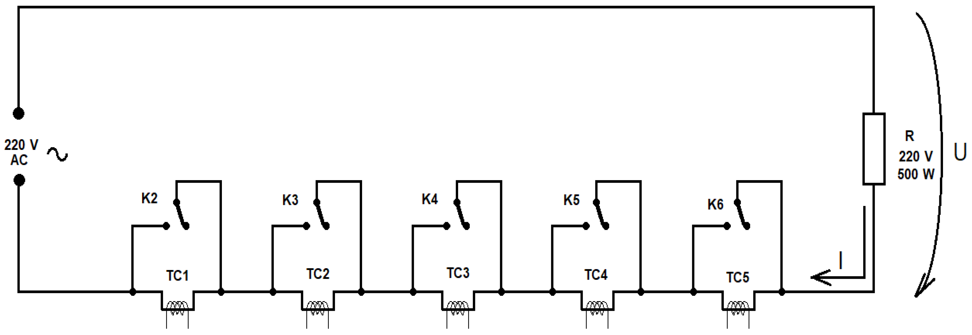
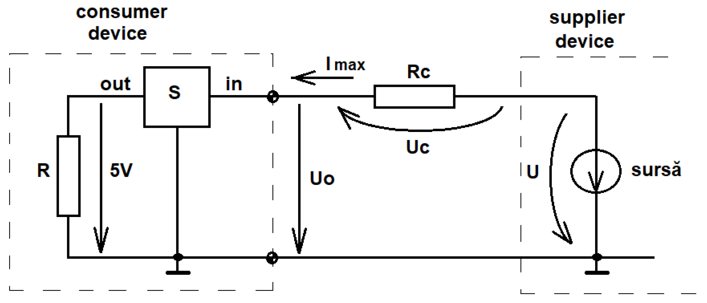
4.3. Issues Related to Remote Powering of Devices

The voltage drops on the cables used in the network are illustrated in Figure 14.

• R—equivalent electrical resistance of the consumer.
• S—voltage stabilizer.
• R_c—equivalent electrical resistance of cables.
• I_max—maximum current absorbed by the consumer.

The voltage source in the supplying device supplies the consumer device with voltage U = 20 V via the mains cables. There is a voltage drop on the supply cables U_c:

$${\mathrm{U}}_{\mathrm{c}}={\mathrm{R}}_{\mathrm{c}}·{\mathrm{I}}_{\mathrm{m}\mathrm{a}\mathrm{x}}$$

(20)

In the electrical circuit in Figure 10, the sum of the voltages is:

$$\mathrm{U}={\mathrm{U}}_{\mathrm{c}}+{\mathrm{U}}_{\mathrm{o}}$$

(21)

The stabilizer S provides a supply voltage of 5 V to the consumer (typical for digital circuits) and needs a minimum input margin of 2 V., i.e., U_o > 7 V (LM7805), for cable length 500 m, R_c = 55 Ω.

$$\mathrm{U}={\mathrm{R}}_{\mathrm{c}}·{\mathrm{I}}_{\mathrm{m}\mathrm{a}\mathrm{x}}+{\mathrm{U}}_{\mathrm{o}}$$

(22)

$${\mathrm{I}}_{\mathrm{m}\mathrm{a}\mathrm{x}}\le \frac{\mathrm{U}-{\mathrm{U}}_{\mathrm{o}}}{{\mathrm{R}}_{\mathrm{c}}}=\frac{20-7}{55}=\frac{13}{55}=0.236\mathrm{A}=236\mathrm{mA}$$

Therefore, at a 500 m network cable length, the maximum current drawn by the consumer device should not exceed 236 mA in order to avoid problems with the supply voltage. The following solutions might be used in order to prevent this situation at cable lengths of over 500 m:

-

increase the supply voltage U > 20 V as the difference U − U_c > 7 V,

-

supplying the consumer device locally with a voltage source closer to it so that the voltage drop U_c is lower,

-

the use of a step-up switching voltage stabilizer which is not affected by the voltage drop at its input.

When monitoring the logic parameters (i.e., electric arc in the cracking reactor, H₂ gas pressure existence), the maximum current consumption I respect the limits (I_max < 175 mA).

When monitoring numerical parameters—i.e., temperatures—the current consumption of the microcontroller and the MAX6675 temperature sensor circuits is about 280 mA. This would mean a voltage drop U_c = 15.4 V, well above the allowed value, and to solve this situation, a solution to increase the supply voltage U = 24 V was chosen.

From (20) and (21), we can write:

$$\mathrm{U}-{\mathrm{U}}_{\mathrm{o}}={\mathrm{U}}_{\mathrm{c}}={\mathrm{R}}_{\mathrm{c}}·{\mathrm{I}}_{\mathrm{m}\mathrm{a}\mathrm{x}}$$

(23)

In order to be able to correctly power the device through the communication network:

$${\mathrm{U}}_{\mathrm{c}}\le \mathrm{U}-{\mathrm{U}}_{\mathrm{o}}$$

(24)

$${\mathrm{R}}_{\mathrm{c}}\le (\mathrm{U}-{\mathrm{U}}_{\mathrm{o}})/{\mathrm{I}}_{\mathrm{m}\mathrm{a}\mathrm{x}}$$

(25)

$$\mathrm{r}·\mathrm{l}\le \left(\mathrm{U}-{\mathrm{U}}_{\mathrm{o}}\right)/{\mathrm{I}}_{\mathrm{m}\mathrm{a}\mathrm{x}} \mathrm{i}.\mathrm{e}., \mathrm{l}\le \left(\mathrm{U}-{\mathrm{U}}_{\mathrm{o}}\right)/\left(\mathrm{r}·{\mathrm{I}}_{\mathrm{m}\mathrm{a}\mathrm{x}}\right)$$

(26)

where, for CAT.5 UTP cable, r < 188 Ω/1000 m:

r—specific electrical resistance in the loop of the communication cable;

l—wire length.

Example: For a networked device powered by 24 V through two wires of the communication cable, having a consumption of 280 mA:

$$\mathrm{l}\le \left(\mathrm{U}-{\mathrm{U}}_{\mathrm{o}}\right)/\left(\mathrm{r}·{\mathrm{I}}_{\mathrm{m}\mathrm{a}\mathrm{x}}\right)=\left(24-7\right)/\left(0.188·0.280\right)=11/0.0526=209.1 \mathrm{m}$$

That means the cable length should not exceed 209 m.

In the technique of remote powering of network devices (POE—Power Over Ethernet), a supply voltage U = 50 V is used, and at the other end of the network, there is a so-called “POE adapter”.

If the adapter contains only plugs and connectors, it is called a passive POE adapter; the voltage stabilization required by the network device is performed inside the adapter.

If the POE adapter also contains a stabilizer or a voltage booster to compensate for voltage drops on the wires, it is called active POE. It is necessary to choose the type of POE adapter according to the power consumption of the networked device. The active POE adapter is more efficient, has lower power losses, and can power devices with higher current consumption that passive adapters cannot handle. However, it is more expensive.

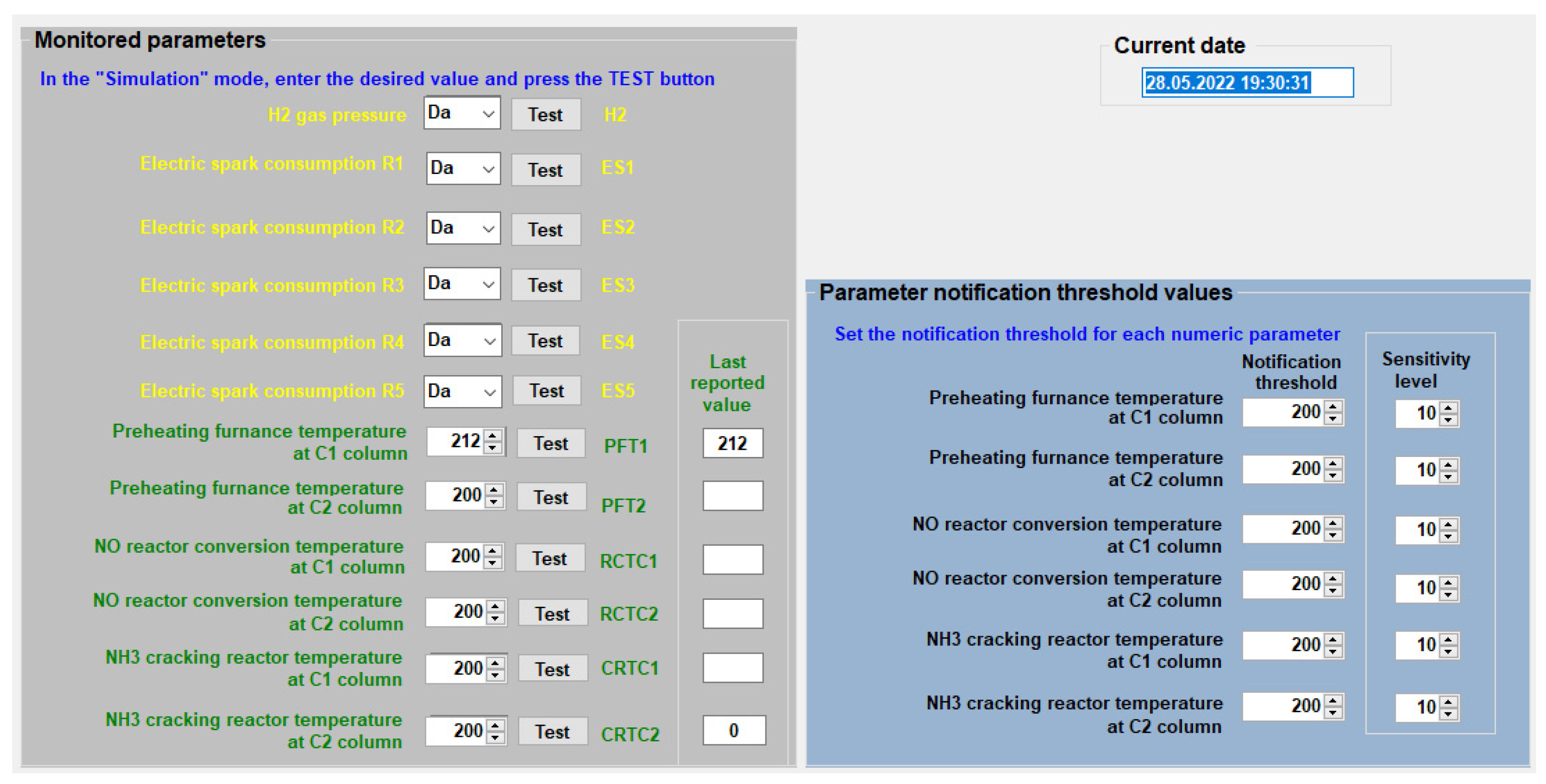
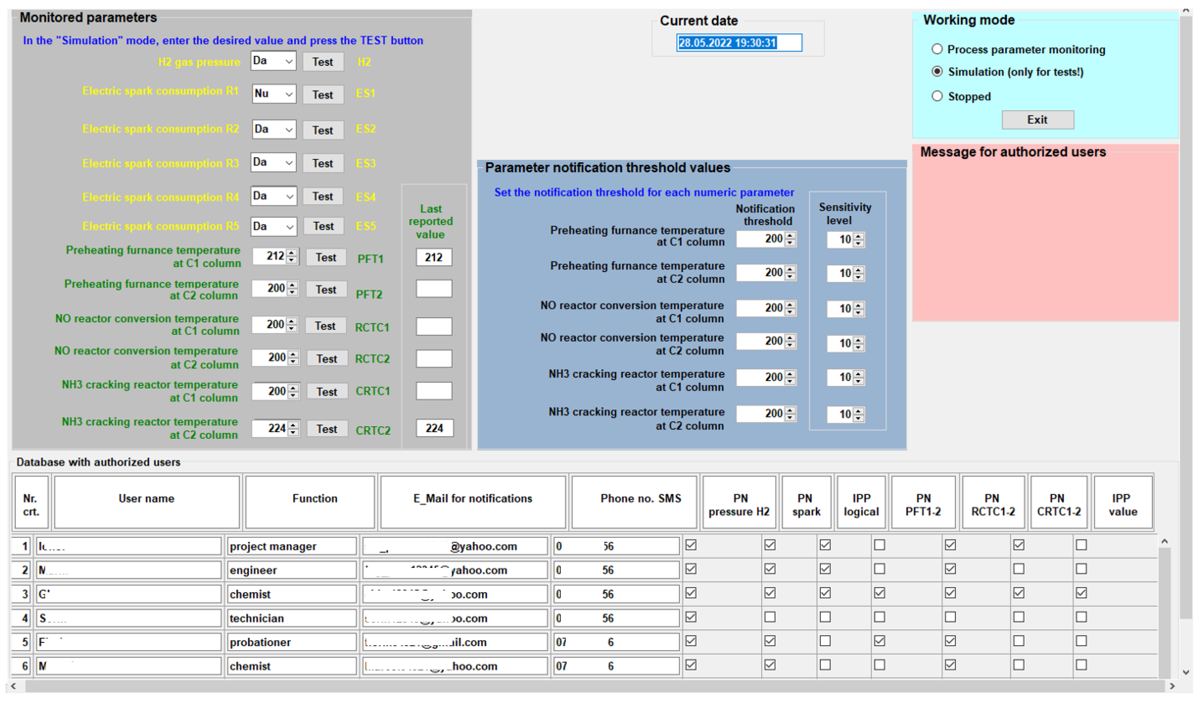
4.4. The Programme for Monitoring the Separation Process of Isotope ¹⁸O Isotope Exchange Reaction

The monitoring program was designed in the Visual Basic 2008 graphical environment (Figure 15) and had three main parts: Acquisition of monitored parameters values, database with hierarchical users and communication with users.

The parameter value acquisition part is responsible for acquiring via USB from the microcontroller the values of the monitored parameters, setting threshold levels for the numerical values and displaying them on the computer screen.

The database contains the name, telephone number, e-mail contact address of the system and the options with rights in the system of each user. The two are connected by the program so that, depending on the values of the parameters, the database is checked, and a standard message is sent by SMS or E-Mail to the users, notified by the options with rights in the system.

At the same time, in reverse, if the authorized user, located somewhere remotely from the process, wants to query the status of the monitored parameters, he sends a message by E-Mail or SMS to the predefined E-Mail address or phone number of the monitoring system, with the text “Query”.

In a short time (about 20 s), the system will reply back to the querying E-Mail address or phone number with a typed message with the values of all parameters for which the querying user is advised.

The program is provided on the top right with a window with three working options:

• “Normal” working mode, in which the monitoring computer receives the monitored parameter values from microcontroller A via the USB port.
• The “simulation” working mode is only used to test the communication of the program with the users; the computer does not receive any more information from the real process.
• Working mode “off”; monitoring does not work.

During the whole operation in modes (2) and (3), the program will display a warning about this.

On the left side in Figure 15, one can see the illustration of a window in which the monitored process parameters are displayed. Parameters marked with yellow are logical (they can take only the value “Yes” or “No”). Parameters marked with green are numerical; in this case, they represent the values of the measured temperatures.

The “Test” button next to each parameter is only valid in “Simulation” mode, when the parameter values can be entered from the keyboard and the corresponding button can be clicked.

In the middle of the screen, in the blue window, you can set threshold values for numerical parameters, for which, once exceeded, the program sends notifications to the users.

At the same time, a sensitivity threshold can be set for each numeric parameter so that the program will not send a notification about a parameter until this threshold is exceeded.

This method has been used to ensure that the program does not send consecutive notifications to users when there is even a minor change in the value of the parameter.

In Figure 16, the database with registered users is represented at the lower end. The important fields for the program are “Crt. no.”, “E-Mail address”, “SMS phone no.” and the checked or unchecked options, which give rights to the respective user.

In the options (rights) category, there are two choices:

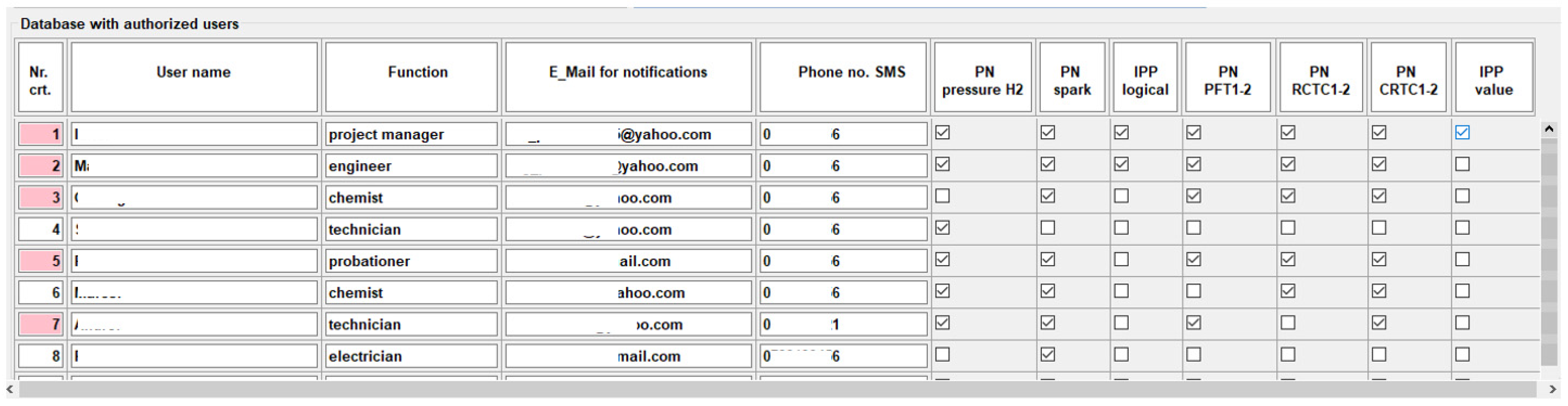
• NP—(Parameter Notification) for the user to be notified when the threshold value of the respective parameter is changed or exceeded.
• PIP—(Permission to Query Parameter) so that the user can ask for the value of the parameter at any time, independently of notification.

Only phone numbers or e-mail addresses registered in the database can access the monitoring program from outside.

The options for each user in the database can be changed at any time.

E-mails are sent via the SMTP server service (Simple Mail Transfer Protocol) and SMS to phone numbers via the Mail to SMS service.

The “Simulation” work mode is very important in preparing the system to work, checking if the E-Mail addresses and phone numbers are correct and if the communication works correctly.

In this mode, all parameters monitored by the program can be tested in turn. One can simulate various logical or numerical values and check whether the program sends the correct notification message to the users.

A Mail or SMS sent by the program is sent simultaneously to all users notified of that notification. Figure 17 presents the monitoring program menu.

In SMTP transmission mode, it should be taken into account that the ISP and SMTP server may reserve the right to limit the number of emails sent from a sender for anti-SPAM reasons. Therefore, this should be negotiated with the provider when implementing the process monitoring system.

4.5. The Results Obtained through the Simulation of the Proposed Mathematical Model

The suggested mathematical model, which represents the separation cascade operation, is simulated in MATLAB/Simulink. The MATLAB programming environment can be installed on the process computer from the structure of the proposed monitoring system. Additionally, it allows the connection with the Process Input Interface, respectively, with the Process Output Interface.

Figure 18 and Figure 19 present the separation cascade responses, more exactly, the responses of the two separation columns from the separation cascade structure. These responses are obtained by simulating the proposed mathematical model in the context in which the imposed value of the ¹⁸O isotope concentration at the SC2 output is 8%. In order to obtain an acceptable energy consumption for the plant, the input flow in SC1 is imposed at the value F₁(t) = 1400 l/h. By running NN5, the value F₂(t) = 118.61 l/h resulted. It is a value Ich, in the absence of disturbances, that ensures the obtaining of the imposed value of the ¹⁸O isotope concentration at the separation cascade output.

Figure 18 shows that the steady-state value of the ¹⁸O concentration at the SC1 output is Z_1st = 1.419%, and from Figure 19 results that the steady-state value of the ¹⁸O concentration at the SC2 output is Z_2st = 8%, which represents the imposed value. Consequently, the efficiency of the proposed modeling solution is proven. In order to analyze the settling time of the two responses, the steady state band of ±1% near the steady state value of the ¹⁸O isotope is defined (for both SC1 and SC2), a band that is appropriate for ensuring the necessary precision. In this context, the settling time of SC1 is t_s1 = 931.7 h, and the settling time of SC2 is t_s2 = 1715.3 h.

An important aspect in the analysis of the separation cascade operation is referring to the study of the influence of the d_β(t) disturbance, more exactly of the influence of the β differentiation order variation. In Figure 20, the comparative graph between the response of the separation cascade (which is assimilated with the response of SC2) and the response of the proposed model is presented in the case when the β differentiation order varies from the initial identified value of 0.92 to the value of 0.73 at the moment t₁ = 2500 h.

The considered variation of β differentiation order is a very consistent one and rarely encountered in practice. As a case study, this high variation of the β parameter is considered in order to prove the high quality of the mathematical model. Figure 20 results that the disturbance has a very aggressive effect on the separation process operation, with the ¹⁸O isotope concentration at the SC2 output decreasing from the value of 8% to the value of 4.24% (in steady state regime; after 1600 h from the disturbance occurrence). Figure 20 also highlights the main advantage of the proposed original model, in particular, the possibility to simulate the online variation of the β(t) differentiation order. Due to this aspect and by using the PIC controller, the mathematical model response from Figure 20 follows with very high accuracy the real response of the separation cascade.

The small oscillations of the proposed mathematical model response which occur immediately after t₁ = 2500 h are due to the control effort generated by the PIC controller in order to follow the response of the real separation cascade through the online variation of the β(t) differentiation order (associated to the model). However, the mentioned oscillations are insignificant regarding the deviations of the model response in comparison with the real separation cascade response. In Figure 21, the variation of the β(t) differentiation order of the proposed model is presented.

The control effort generated by the PIC controller is visible immediately after t₁ = 2500 h (the moment when the parametric disturbance occurs in the separation process operation), being characterized through the consistent oscillations from Figure 21. After 121.4 h from the occurrence of the disturbance, the β(t) differentiation order gets steady to the value of 0.73, which is exactly the decreased value of β due to the parametric disturbance occurrence. Consequently, the online identification of the new value of the β parameter is the correct one.

Another essential aspect relates to the rejection of the previously presented parametric disturbance effect. As shown in Figure 6, the compensation procedure is based on the usage of NN2, NN3 and NN4 neural networks, respectively, on the generation of FC(t) and implicitly F_2C(t) compensation signals. By applying this strategy, the separation cascade responses from Figure 22 are obtained.

The NN4 neural network generates at the output the value of the compensation signal F_2C = 21.39 L/h, resulting in a total input nitric oxides flow in SC2 of F₂(t) = 140 L/h. This value is the correct one because, according to Figure 4, it implies the lowest HETP₂(F₂) value which also implies the highest separation of SC2 and the highest value of the ¹⁸O isotope at the SC2 top. However, due to the fact that the considered disturbance has a high value (Δβ = −0.19), this compensation is not enough, and the solution, in this case, is to adjust the value of the F₁(t) input flow in SC1. Based on (5) but using its adapted form for obtaining the F₁(t) nitric oxide flow, the compensation signal F_1C(t) = 197.8 L/h results. By using the two compensation flows F_1C(t) and F_2C(t) at the mentioned values, Figure 21 results that the considered parametric disturbance effect is rejected (the ¹⁸O isotope concentration reaches again, in steady state regime, the imposed value of 8%, after 2483.8 h from the moment of the disturbance occurrence). Additionally, by using the compensation through the adjustment of the K_I(β(t)) signal value, the response of the suggested mathematical model follows with high accuracy the response of the separation cascade in the disturbance rejecting regime, the proof of the proposed model quality, correctness and accuracy being made again.

The compensation effort used in the case of the disturbance effect rejection inside the internal structure of the model is highlighted in Figure 23, in which the variation of the K_I(β(t)) is presented.

As shown in Figure 23, after the moment t₁ = 2500 h when the disturbance occurs, the K_I(β(t)) varies from the initial compensation value of 1.512 [-] to the value of 2.904 [-] in order to compensate the disturbance effect. The stabilization at the new value of 2.904 [-] is obtained after 121.4 h from the disturbance occurrence, an aspect which is obvious due to the fact that K_I is a function of β(t) and according to Figure 21, β(t) gets steady after 121.4 h from t₁ = 2500 h. The consistent oscillations of the K_I signal immediately after the occurrence of the disturbance are due to the same dependency of K_I on β(t).

In order to test the robustness of the model, the second disturbance is introduced. This disturbance occurs at the moment t₂ = 5000 h from the simulation start and consists in doubling the value of the b₁ constant from (14), which is also an aggressive disturbance. In this case, the comparative graph between the separation cascade response and the response of the proposed mathematical model is presented in Figure 24.

In Figure 24, the case of not compensating for the effect of the first type of disturbance (d_β(t)) but compensating for the effect of the second type of disturbance is considered. In the proposed mathematical model structure, the ¹⁸O isotope concentration decrease after the t₂ moment is interpreted as the effect of the β(t) decrease and due to the cumulative actions of the PIC controller and of the compensation system (containing the NN2, NN3 and NN4 neural networks), the effect of the second type of disturbance is rejected (after 4523.7 h from the moment t₂, the ¹⁸O concentration reaches the steady state value equal to its steady state value from before the second type of disturbance occurrence). Additionally, the model response, in this case, too, follows with high accuracy the response of the separation cascade. An important aspect that has to be mentioned is that, based on the proposed model and compensation algorithm, the compensation for the effects of both types of disturbances can be made simultaneously.

5. Conclusions and Further Developments

Productive ¹⁸O isotope separation systems by isotope exchange between NO and HNO₃ solution are highly complex, non-linear chemical processes with many input and output parameters.

These systems operate with toxic, corrosive gases and solutions (NO, NO₂, HNO₃, NaOH) and also with flammable gases under pressure (H₂).

The process of obtaining a semi-effective amount of isotope can take months, with significant consumption of raw material, energy and production costs.

There are some important points in the system where any failure, disturbance or neglect of parameter values would endanger the steady-state operation of the plant, would result in the destruction of the separation effort performed to date, and the column would practically return to its original state with significant losses.

The parameters monitored may be non-physical process parameters (e.g., separation column temperature, pressure, or product concentrations) or maybe parameters of secondary systems serving the main process.

The operation of this installation is spread over large areas; the personnel supervising the operation must keep a safe distance from pressure vessels, which are explosive or easily flammable.

For these reasons, remote monitoring of these important system parameters is necessary.

The monitoring points of the separation process chosen, i.e., the six logical parameters and six numerical parameters (approached as case studies), are important both for the operational safety of the plant and for avoiding an ultimate compromise of the final product.

For the manager of the separation plant, the head of the department and his superiors, who can remotely monitor the process, this information can be enlightening in making decisions regarding the proper functioning of the isotope production system.

Thermocouple temperature sensors have good linearity (1 mV/100 °C) and a wide measuring range (1500 °C), but the signal level provided is very low, and they need a specialized integrated circuit to amplify and continue to transmit the signal.

It is necessary to adapt the communication interface to the type of specialized circuit and the type of interface with which it is equipped.

If the reading of the signal delivered by the specialized circuit is in the immediate vicinity of the specialized circuit, interfaces operating over short distances may also be used, and a long-distance communication interface shall be used in order to further transmit the value.

The RS485 interface is best suited for a remote parameter monitoring and transmission interface. It is very versatile, easy to implement, has good immunity to disturbances, can connect multiple devices (ModBus mode) and can communicate over long distances (up to 1200 m).

When remotely powering networked devices via the communication network cable, problems can occur in relation to the current drawn by the device and voltage drop on the wires if the wires are long.

To pre-empt these problems, one solution is to make the supply voltage high enough to compensate for this voltage drop and supply the network device with the required voltage.

Another solution is to use a step-up switching voltage stabilizer at the end of the network so that the voltage at the terminals of the network device can be raised to the nominal value.

Remote process monitoring first appeared on PSTN fixed telephone networks and was introduced on the security system manufacturers’ market for remote signaling of events. Subsequently, with the development of the electronics industry and communication technology, it was also adapted for Smart-Building systems for remote management of environmental parameters in a building, with communication via GSM telephone network or via Internet, LAN, and Wi-Fi.

Trends in remote process monitoring communications are to use IP communicators in particular.

Basically, in this case, the monitoring computer is connected via LAN and Wi-Fi to the Internet, and the role of the IP communicator is taken over by the monitoring software running on the computer.

On the experimental board, one tried to simulate the circuitry of an interface under field conditions. The eventual implementation of this interface could be performed with minor modifications.

The monitoring system allows the researchers and the operators to acquire experimental data from the real plant operation. As evinced in this manuscript, the experimental data can be used for determining the mathematical model which describes the separation plant operation. The proposed original mathematical model is run on the process computer from the structure of the monitoring system in parallel with the real plant. Consequently, the online identification of the variations of some structural parameters of the separation process can be made, and consequently, the operators can make the appropriate decisions in order to maintain the operation of the separation cascade in the imposed operation regimes. The mathematical model of the separation plant is implemented considering the fact that the final separation column from the separation cascade structure has a fractional-order behavior. In order to have the possibility to implement and simulate the proposed mathematical model on the process computer, several neural networks are used to learn the dynamics of the non-linear parameters from the model structure. The simulation results prove the feasibility of implementing the proposed monitoring strategy augmented with a model-based decision machine which assists the operators in the separation plant exploitation.

The parametric errors affected some signals significantly, and in the case of other signals, they had an insignificant effect. For example, in the case of HETP functions, the parametric errors are insignificant because all the associated measurements are made in a steady state regime, and the measurements were repeated during the steady state regime (which, in general, has a long duration). In the case of the dynamic responses (the experimental responses from Figure 2 and Figure 5), the parametric errors have a significant impact due to the fact that the corresponding measurements are made in the transitory regime, an aspect which implies several problems, as the measurement moment is relative, the measurement sample is taken in the case when the concentration is not steady, or the possibility to verify the correction of the measurements through repetition is restrictive.

However, the effect of these parametric disturbances was eliminated to a high degree through the deduction of the most probable response generated through the simulation of the proposed mathematical model (Figure 5). This response „averages” with good performances in the experimental response. As a synthesis of the previous remarks, the parametric errors could have an effect only in the identification of the plant time constants, but they do not have a significant effect in the identification of the plant steady-state regime (it is implied by the HETP functions). However, even in the case of the time constant, due to the applied modeling procedure, the possible effect of the parametric errors is limited, and it can be rejected by using a control strategy. The effect of other types of possible parametric errors can be simulated using the proposed model due to the possibility of the variation of the process fractional differentiation order.

Some of the possible future directions of development that could be addressed in the field of the present application are:

• Expanding the number of remotely monitored parameters, possibly adding some parameters that are not of the isotope production process but of systems that serve the process (e.g., thermal switches, monitoring of their supply voltage value, smoke sensor, gas sensor, etc.).
• Modification of the communication protocol so that the communication interface can detect if the network cable is interrupted or if a network device is not responding (interrupted, disconnected) and communicate this to the monitoring computer.
• Development of a more complex monitoring program with a graphical display (possibly in the LabVIEW environment)
• Development of a client application for users’ mobile devices containing intuitive graphics of the system and monitoring parameters
• Extending the experimental part to the entire installation
• The implementation of an advanced control strategy for the automatic control of all the parameters which occur in the separation cascade operation.
• The implementation, based on the proposed mathematical model, of an optimization system of the separation cascade energy consumption.
• The extension of the proposed mathematical model by considering, also, as a control signal, the temperature in the column (the temperature can be modified through the corresponding control system); the temperature variation would imply the variation of the α elementary separation factor.

References

1. Codoban, A.; Abrudean, M.; Silaghi, H.; Dale, S.; Mureşan, V.; Fișcǎ, M.; Ungureşan, M.L.; Cordoş, R. Monitoring System of Production Installation for the Separation of Isotope 18O. In Proceedings of the 2021th International Conference on Engineering of Modern Electric Systems (EMES), Oradea, Romania, 10–11 June 2021. [Google Scholar]
2. Okahashi, N.; Yamada, Y.; Iida, J.; Matsuda, F. Isotope Calculation Gadgets: A Series of Software for Isotope-Tracing Experiments in Garuda Platform. Metabolites 2022, 12, 646. [Google Scholar] [CrossRef] [PubMed]
3. Wang, Y.; Chen, D.; Augusto, R.; Liang, J.; Qin, Z.; Liu, J.; Liu, Z. Production Review of Accelerator-Based Medical Isotopes. Molecules 2020, 27, 5294. [Google Scholar] [CrossRef] [PubMed]
4. Hou, C.; Tian, D.; Xu, B.; Ren, J.; Hao, L.; Chen, N.; Li, X. Use of the stable oxygen isotope method to evaluate the difference in water consumption and utilization strategy between alfalfa and maize fields in an arid shallow groundwater area. Agric. Water Manag. J. 2021, 256, 107065. [Google Scholar] [CrossRef]
5. Stephens, J.A.; Ducea, M.N.; Killick, D.J.; Ruiz, J. Use of non-traditional heavy stable isotopes in archaeological research. J. Archaeol. Sci. 2021, 127, 105334. [Google Scholar] [CrossRef]
6. Vasaru, G. (Ed.) Izotopii Stabili; Editura Tehnica: București, Romania, 1968. [Google Scholar]
7. Abrudean, M.; Ungureșan, M.; Pica, E.-M. Preliminaries Concerning the Modeling of the Absorption Process of Nitrogen Oxides in Aqueous Nitric Acid. In Proceedings of the A&Q’98 International Conference of Automation and Quality Control, Cluj-Napoca, Romania, 28–29 May 1998. [Google Scholar]
8. Khoroshilov, A.V. Production of stable isotopes of light elements: Past, present and future. J. Phys. Conf. Ser. 2018, 1099, 012002. [Google Scholar] [CrossRef]
9. Love, J. Process Automation Handbook—A Guide to Theory And Practice; Springer: London, UK, 2007. [Google Scholar]
10. Mureșan, V.; Abrudean, M.; Ungureșan, M.L.; Coloși, T. Modeling and simulation of the isotopic exchange for 18O isotope production. In Proceedings of the 2018 IEEE International Conference on Automation, Quality and Testing, Robotics (AQTR), Cluj-Napoca, Romania, 24–26 May 2018. [Google Scholar]
11. Abrudean, M.; Unguresan, M.L.; Silaghi, H.; Muresan, V.; Codoban, A. Experimental Identification of the C-13 Isotope Separation Process by Cryogenic Distillation on a Two-Column Separation Cascade. In Proceedings of the 2019 15th International Conference on Engineering of Modern Electric Systems (EMES), Oradea, Romania, 13–14 June 2019. [Google Scholar]
12. Codoban, A. Monitorizarea de la Distanță a Parametrilor Procesului de Separare a Izotopului 18O. Ph.D. Thesis, University of Oradea, Oradea, Romania, 2021. [Google Scholar]
13. Niazi, M.; Protocols for Industrial Remote Monitoring. Control Automation. 3 May 2021. Available online: https://control.com/technical-articles/protocols-for-industrial-remote-monitoring/ (accessed on 14 May 2022).
14. Saxena, S.C.; Taylor, T.I. Enrichement of oxygen-18 by the chemical exchange of nitric oxide with nitric acid solution. J. Chem. Phys. 1962, 66, 1480–1487. [Google Scholar] [CrossRef]
15. Axente, D.; Abrudean, M.; Baldea, A. Separation of 15N, 18O, 10B, 13C through Isotopic Exchange; Editura Casa Cărţii de Ştiinţă: Cluj-Napoca, Romania, 1995; pp. 249–263. ISBN 973-9654-4-3. [Google Scholar]
16. Abrudean, M.; Axente, D.; Bâldea, A. Enrichment of 15N and 18O by chemical Exchange Reaction between Nitrogen Oxides (NO, NO2) and Aqueous Nitric Acid. Isotopenpraxis 1981, 17, 377–382. [Google Scholar] [CrossRef]
17. Doyle, J.; Carroll, J. Routing TCP/IP; ciscopress.com: Indianapolis, IN, USA, 2005; Volume I. [Google Scholar]
18. Carroll, J.; Doyle, J. Routing TCP/IP: CCIE Professional Development; ciscopress.com: Indianapolis, IN, USA, 2016; Volume II. [Google Scholar]
19. Stephens, R. Begin Database Design W/WS; Josey-Bass: Hoboken, NJ, USA, 2008. [Google Scholar]
20. Kassi, S.; Karlovets, E.V.; Tashkun, S.A.; Perevalov, V.I.; Campargue, A. Analysis and theoretical modeling of the 18O enriched carbon dioxide spectrum by CRDS near 1.35 μm: (I) 16O 12C 18O, 16O 12C 17O, 12C 16O2 and 13C 16O2. J. Quant. Spectrosc. 2017, 187, 414–425. [Google Scholar] [CrossRef]
21. Dulf, E.; Kovacs, L. Fractional order control of the cyber-physical cryogenic isotope separation columns cascade system. In Proceedings of the 2018 IEEE International Conference on Automation, Quality and Testing, Robotics (AQTR), Cluj-Napoca, Romania, 24–26 May 2018. [Google Scholar]
22. Mureşan, V.; Abrudean, M.; Ungureşan, M.-L.; Clitan, I.; Coloşi, T. Control of the 18O isotope separation process. In Proceedings of the SACI, Timisoara, Romania, 12–14 May 2016; pp. 283–288. [Google Scholar]
23. Monje, C.A.; Chen, Y.; Vinagre, B.M.; Xue, D.; Feliu, V. Fractional-order systems and controls. In Fundamentals and Applications; Springer: New York, NY, USA, 2010; pp. 3–9. [Google Scholar]
24. Lin, W.C.; Tsai, C.F.; Zhong, J.R. Deep learning for missing value imputation of continuous data and the effect of data discretization. Knowl. Based Syst. 2022, 239, 108079. [Google Scholar] [CrossRef]
25. Chen, L.; Chen, P.; Lin, Z. Artificial Intelligence in Education: A Review. IEEE Access 2020, 8, 75264–75278. [Google Scholar] [CrossRef]
26. Haykin, S. Neural Networks and Learning Machines, 3rd ed.; Pearson Education, Inc.: Upper Saddle River, NJ, USA, 2009; pp. 818–845. [Google Scholar]
27. Kamra, A.; Bhambri, P. Computer Peripherals and Interfaces; Technical Publications Pune: Maharashtra, India, 2008. [Google Scholar]
28. System Identification. Available online: https://www.libristo.ro/ro/carte/system-identification_01210326?utm_source=google&utm_medium=surfaces&utm_campaign=shopping%20feed&utm_content=free%20google%20shopping%20clicks%20merchant_ro&gclid=EAIaIQobChMI6e6Ywt3o_QIVoQYGAB3ymgCeEAQYBCABEgI7yfD_BwE (accessed on 14 May 2022).
29. Experimental Techiques—Developments, Applications and Tutorials in Experimental Mechanics and Dynamics. Available online: https://www.springer.com/journal/40799?gclid=EAIaIQobChMI4pCO67_p_QIVhdZ3Ch0q-wTuEAAYASAAEgJVDfD_BwE (accessed on 20 May 2022).
30. Identification and Classical Control of Linear Multivariable Systems. Available online: https://www.enbook.ro/catalog/product/view/id/2052104?gclid=EAIaIQobChMI6e6Ywt3o_QIVoQYGAB3ymgCeEAQYCSABEgKu1_D_BwE (accessed on 22 July 2022).
31. Models and Methods for Parametric Identification. Available online: https://link.springer.com/chapter/10.1007/978-1-4471-3848-8_11 (accessed on 12 September 2022).
32. System Identification—Second Edition. Available online: https://www.libristo.ro/ro/carte/system-identification-second-edition_20173614 (accessed on 18 July 2022).
33. Using the SDP Identification Method for Electromechanical Systems. Available online: https://reader.elsevier.com/reader/sd/pii/S2405896321012362?token=D86A95AE58908882F60600129D3AA110A55E7645BE23C1CA61D838465FAC13116767A4EAB2E654E62B9E980950183B85&originRegion=eu-west-1&originCreation=20230319193608 (accessed on 20 October 2022).
34. Nonlinear System Identification. Available online: https://www.libristo.ro/ro/carte/nonlinear-system-identification_06829824 (accessed on 17 November 2022).
35. Karimov, A.I.; Kopets, E.; Nepomuceno, E.G.; Butusov, D. Integrate-and-Differentiate Approach to Nonlinear System Identification. Mathematics 2021, 9, 2999. [Google Scholar] [CrossRef]
36. Obeid, S.; Ahmadi, G.; Jha, R. NARMAX Identification Based Closed-Loop Control of Flow Separation over NACA 0015 Airfoil. Fluids 2020, 5, 100. [Google Scholar] [CrossRef]
37. Gedon, D.; Wahlström, N.; Schön, T.B.; Ljung, L. Deep state space models for nonlinear system identification. IFAC-PapersOnLine 2021, 54, 481–486. [Google Scholar] [CrossRef]
38. Huffaker, R.; Bittelli, M.; Rosa, R. Phase–Space Reconstruction, Chapter 3. In Nonlinear Time Series Analysis with R; Oxford Academic: Oxford, UK, 2017. [Google Scholar]
39. Tian, R.; Yang, Y.; van der Helm, F.C.; Dewald, J. A novel approach for modeling neural responses to joint perturbations using the NARMAX method and a hierarchical neural network. Front. Comput. Neurosci. 2018, 12, 96. [Google Scholar] [CrossRef] [PubMed]
40. Yang, L.; Liu, J.; Yan, R.; Chen, X. Spline adaptive filter with arctangent-momentum strategy for nonlinear system identification. Signal Process. 2019, 164, 99–109. [Google Scholar] [CrossRef]
41. Torres, L.; Besancon, G.; Verde, C.; Georges, D. Parameter identification and synchronization of spatio-temporal chaotic systems with a nonlinear observer. IFAC-PapersOnLine 2012, 45, 267–272. [Google Scholar] [CrossRef]
42. Gao, Z.; Chen, M.Z.Q.; Zhang, D. Special Issue on “Advances in Condition Monitoring, Optimization and Control for Complex Industrial Processes”. Processes 2021, 9, 664. [Google Scholar] [CrossRef]
43. Gao, Z.; Liu, X. An overview on fault diagnosis, prognosis and resilient control for wind turbine systems. Processes 2021, 9, 300. [Google Scholar] [CrossRef]
44. Xu, S.; Hashimoto, S.; Jiang, W.; Jiang, Y.; Izaki, K.; Kihara, T.; Ikeda, R. Slow mode-based control method for multi-point temperature control system. Processes 2019, 7, 533. [Google Scholar] [CrossRef]
45. Trimmer, W. Understanding and Servicing Alarm Systems; Butterworth-Heinemann: Oxford, UK, 1999. [Google Scholar]
46. Blum, J. Exploring Arduino: Tools and Tehniques for Engineering Wizardry; Wiley: Hoboken, NJ, USA, 2013. [Google Scholar]
47. Margolis, M. Arduino Cookbook; O’Reilly Media: Newton, MA, USA, 2011. [Google Scholar]
48. *** Data Transmission Circuits-Line Circuits; Texas Instruments: Dallas, TX, USA, 1996.
49. Dong, Y.; Wang, S.; Liu, H. Establishment of Remote Measure and Control System Based on Complex Dynamic Objects. In Proceedings of the 2009 9th International Conference on Electronic Measurement and Instruments, (ICEMI), Beijing, China, 16–19 August 2009. [Google Scholar]
50. Codoban, A.; Abrudean, M.; Cordoş, R.; Mureşan, V.; Fișcă, M.; Ungureşan, M.L.; Silaghi, H.; Spoială, V. Preliminaries Regarding the Monitoring of the Parameters of a Separation Cascade for Isotope 18O. In Proceedings of the 2021th International Conference on Engineering of Modern Electric Systems (EMES), Oradea, Romania, 10–11 June 2021. [Google Scholar]
51. Bockmann, C.J.; Klander, L.; Tang, L. Visual Basic Programmer’s Library; Jamsa Pr: Phoenix, AZ, USA ; State University of Pennsylvania: State College, PA, USA, 1998. [Google Scholar]
52. Berry, M.V.; Lewis, Z.V. On the Weierstrass-Mandelbrot fractal function. Proc. R. Soc. Lond. A Math. Phys. Sci. 1980, 370, 459–484. [Google Scholar]
53. Guariglia, E.; Silvestrov, S. Fractional-Wavelet Analysis of Positive definite Distributions and Wavelets on D’(C). In Engineering Mathematics II; Rancic, S., Ed.; Springer: Berlin/Heidelberg, Germany, 2016; pp. 337–353. [Google Scholar]
54. Yang, L.; Su, H.; Zhong, C.; Meng, Z.; Luo, H.; Li, X.; Tang, Y.; Lu, Y. Hyperspectral image classification using wavelet transform-based smooth ordering. Int. J. Wavelets Multiresolut. Inf. Process 2019, 17, 1950050. [Google Scholar] [CrossRef]
55. Guariglia, E. Fractional calculus, zeta functions and Shannon entropy. Open Math. 2021, 19, 87–100. [Google Scholar] [CrossRef]
56. Zheng, X.; Tang, Y.; Zhou, J. A Framework of Adaptive Multiscale Wavelet Decomposition for Signals on Undirected Graphs. IEEE Trans. Signal Process. 2019, 67, 1696–1711. [Google Scholar]
57. Guariglia, E.; Guido, R. Chebyshev wavelet analysis. J. Funct. Spaces 2022, 2022, 5542054. [Google Scholar] [CrossRef]
58. Automatic Control Systems. Available online: https://www.fruugo.ro/sisteme-de-control-automat-editia-a-zecea-de-farid-golnaraghibenjamin-kuo/p-48829124-97007997?language=ro&ac=KelkooCSS&gclid=EAIaIQobChMIuK7TneDo_QIVTAWLCh3hgg8lEAQYAyABEgLA2_D_BwE (accessed on 6 June 2022).
Figure 1. The main elements of the considered separation cascade (with explanation in the text).
Processes 11 01594 g001
Figure 2. The experimental step response of the separation cascade (with an explanation in the text).
Processes 11 01594 g002
Figure 3. The HETP1(F1) function variation was experimentally determined.
Processes 11 01594 g003
Figure 4. The HETP2(F2) function variation was experimentally determined.
Processes 11 01594 g004
Figure 5. The graph compares the separation cascade’s experimental reaction and the suggested model’s response.
Processes 11 01594 g005
Figure 6. The implementation of the proposed mathematical model.
Processes 11 01594 g006
Figure 7. Block diagram of a computer system for automatic control of a technological process.
Processes 11 01594 g007
Figure 8. Block diagram of a computer system for automatic control of a technological process with remote monitoring.
Processes 11 01594 g008
Figure 9. Monitoring interface for the 18O isotope manufacturing process diagram.
Processes 11 01594 g009
Figure 10. Current consumption simulation in the cracking reactors.
Processes 11 01594 g010
Figure 11. Experimental system photo.
Processes 11 01594 g011
Figure 12. Simulation of long electric network UTP cables.
Processes 11 01594 g012
Figure 13. Simulation of an RS485 bus with a length of about 500 m via one wire (a) and via two pairs of twisted cables (b).
Processes 11 01594 g013
Figure 14. Wiring diagram of the device.
Processes 11 01594 g014
Figure 15. Parameter values display.
Processes 11 01594 g015
Figure 16. Database of registered users.
Processes 11 01594 g016
Figure 17. Monitoring program menu.
Processes 11 01594 g017
Figure 18. The response of SC1 was obtained by simulating the proposed mathematical model.
Processes 11 01594 g018
Figure 19. The response of SC2 was obtained by simulating the proposed mathematical model.
Processes 11 01594 g019
Figure 20. The effect of the β differentiation order variation.
Processes 11 01594 g020
Figure 21. The variation of the β(t) differentiation order.
Processes 11 01594 g021
Figure 22. The dβ(t) disturbance effect rejection.
Processes 11 01594 g022
Figure 23. The KI(β(t)) compensation signal variation.
Processes 11 01594 g023
Figure 24. The effect of the second type of disturbance.
Processes 11 01594 g024