
Optimal Degradation-Aware Control Using Process-Controlled Sparse Bayesian Learning

Department of Electronics, Mathematics and Sciences, University of Gävle, 80176 Gävle, Sweden
*
Author to whom correspondence should be addressed.
Processes 2023, 11(11), 3229; https://doi.org/10.3390/pr11113229
Submission received: 13 October 2023
/
Revised: 12 November 2023
/
Accepted: 13 November 2023
/
Published: 15 November 2023
(This article belongs to the Special Issue Dynamics Analysis and Intelligent Control in Industrial Engineering)
Abstract
:Efficient production planning hinges on reducing costs and maintaining output quality, with machine degradation management as a key factor. The traditional approaches to control this degradation face two main challenges: high costs associated with physical modeling and a lack of physical interpretability in machine learning methods. Addressing these issues, our study presents an innovative solution focused on controlling the degradation, a common cause of machine failure. We propose a method that integrates machine degradation as a virtual state within the system model, utilizing relevance vector machine-based identification designed in a way that offers physical interpretability. This integration maximizes the machine’s operational lifespan. Our approach merges a physical machine model with a physically interpretable data-driven degradation model, effectively tackling the challenges in physical degradation modeling and accessibility to the system disturbance model. By embedding degradation into the system’s state-space model, we simplify implementation and address stability issues. The results demonstrate that our method effectively controls degradation and significantly increases the machine’s mean time to failure. This represents a significant advancement in production planning, offering a cost-effective and interpretable method for managing machine degradation.
1. Introduction
Production planning and control (PPC) plays a crucial role in mitigating disruptions such as machine failures within manufacturing organizations [1]. Machine failures, particularly those classified as “soft failures”, often arise due to the gradual and irreversible damages accrued during operation [2]. An inaccurate model of a machine’s degradation trajectory can lead not only to erroneous fault predictions but also to eventual machine failures. Ultimately, unpredicted failures can result in various undesirable expenses, including the costs of lost production, wasted materials, and products [3].
The field of predictive maintenance has engaged in comprehensive discussions about fault protection, generally viewing it from two unique perspectives. The first of these perspectives takes a macro approach (high-level), focusing on broader policymaking strategies such as optimizing maintenance through reliability analysis. Typically, this method views the system and its various subsystems as interconnected, unified entities. In contrast, the second perspective adopts a micro approach (low-level), concentrating on improving the field machines’ functionalities. The main aim here is to enhance the availability of field machinery and to accurately estimate the state of health (SoH) of the machinery involved.
The primary focus of high-level reliability analysis and maintenance optimization is to avoid system failure by determining the optimal time for maintenance based on different existing constraints. Most of these approaches employ statistical or mathematical models to substitute the physical model of deterioration to estimate the reliability of the system [4]. For instance, the authors in [5] proposed a method for the optimization of condition-based maintenance for systems under random shocks by optimizing the inspection times according to the system reliability reduction after each shock. In [6], the maintenance planning was optimized in accordance with maintenance resource constraints by deploying non-periodic inspections and minimizing the expected total cost per unit of the failure or repair. In [7,8], the authors proposed maintenance strategies for the optimization of different criteria, e.g., the maximization of availability or minimization of the maintenance cost, for the maintenance systems with constraints on resources and capacity.
Although these methods optimize maintenance based on various constraints, they have strong assumptions about the degradation models or accessibility of some data, making their results exclusive to particular problems. Additionally, the use of mathematical and statistical models replaces the direct relationship between the system’s structure and its degradation with data-driven statistics, bypassing the need for physically interpretable data [9,10,11]. This means that, despite the cost-saving benefits of this simplification by eliminating physical modeling, which is an expensive task, this method hinders the ability to reason based on cause-and-effect relationships that physical reasoning provides. This approach implies that the system’s reliability is influenced by obscure or, at most, partially understood processes that can only be approximated rather than enhanced or controlled. In this way, systems cannot actively support high-level decisions, such as delaying or scheduling failures, by taking optimal actions in the field machines.
On the other hand, with a low-level reliability analysis, the focus is on enhancing the accuracy of the SoH estimation for a single machine as a physical entity. This is usually accomplished by modeling the degradation in the system using different methods. For example, refs. [12,13] used a knowledge-based method, refs. [14,15,16,17] used physical modeling, and [18,19,20,21,22] used data-driven methods for the SoH estimation or remaining useful life (RUL) prediction. Additionally, several studies have proposed methods for controlling the degradation in the machines by either physically modeling the dynamics of the system and its respective degradation [23,24,25,26] or using data-driven methods for estimating the physical parameters of the machine and its degradation [27,28,29,30].
However, to achieve a more comprehensive and flexible PPC, high-level policymaking methods should incorporate these low-level methods and work as an integrated method. Nonetheless, two reasons make existing low-level reliability analysis methods exclusive and only adaptable to some high-level decision making methods. First, these methods try to fit the system’s degradation into predefined mathematical or physical templates, which is a strong assumption as degradation patterns may differ across parts of the system or may not even adhere to any recognizable mathematical form [31,32]. Second, similar to the high-level methods, by discarding the physical model and using machine learning methods [33,34,35], the connection to the physics of the system is not established, and valuable information regarding the type of degradation and the eventual fault is lost.
Given the gap between high-level decision making methods and low-level machine-specific actions, the central question is whether it is possible to support high-level decisions by implementing low-level actions such that machines reach a predetermined maintenance level at the desired time.
In order to do so, the degradation in the machines must be controlled. This requires accurate identification of the relationship between degradation and machine, and proper design of the controller. The authors of [36] showed that degradation in the system can be observed through the residuals of the system’s mathematical model and its physical model. The physical relationship between degradation and system dynamics was later established in [37,38]. Here, the system was considered observable and the damage was considered an unobservable state. Following this, several researchers proposed different methods to address controller and actuator degradation under various constraints. A variable structure controller was designed in [39] to manage different performance challenges and failures. An integrated fault detection, diagnosis, and reconfigurable control scheme was presented in [40]. Methods to handle uncertainty and unobservability in degradation control were introduced in [41] for linear systems and discussed in [42] for non-linear and singular systems. Moreover, a method for degradation control of systems with non-linearities and missing data was suggested in [43].
Examining the evolution path, studies on degradation control generally adopt two primary approaches. Methods like those presented in [44,45] employ a robust control scheme to counteract the degradation and inefficiency of actuators. Conversely, methods such as those in [38,46] leverage the physical model of degradation when designing controllers. The main challenge for both sets of methods is their stringent assumptions regarding the degradation model, disturbances, and accessibility.
To address the challenges in degradation control, this paper proposes a method for controlling degradation by modifying optimal control schemes. Controlling degradation results in longer mean time to failure (MTTF) and reduced maintenance costs by minimizing downtimes or rerouting faults from expensive system components to more economical ones. This study controls degradation by defining it as a new virtual, controllable state of the system. This approach tackles the challenges associated with assumptions about the degradation model, encountered in physical modeling of degradation or inaccessibility to disturbances and the degradation model as faced by robust controllers. These issues are addressed using the sparse Bayesian learning method, which empirically identifies the degradation model using the system’s historical data. Furthermore, the mathematics of machine degradation are studied comprehensively to determine the means of incorporating degradation behavior into the system dynamics.
The remainder of the paper is organized as follows. Section 2 introduces the methodology of the proposed approach. Section 3 explains the procedure used for the simulation of the method. Section 4 presents the results and validation process, while Section 5 discusses the advantages and disadvantages of the method. Finally, conclusions are presented in Section 6.
2. Materials and Methods
In the proposed method, machine degradation is controlled through a four-step process. Initially, the degradation is detected, followed by the identification of the dynamics of degradation via process-controlled learning, which maps the degradation into the system’s states and inputs. Subsequently, these dynamics are incorporated into the model of the system. Finally, control is exerted over the degradation while simultaneously maintaining the quality of the output.
2.1. State-Space Mode and Degradation
The state-space mode (SSM) can be written as follows:
where x includes the system state(s), u is system input(s), A and B represent the physical system parameters (considered constant in time-invariant systems), C is the relationship between the output(s) and state(s) of the system, z is the controlled output, M configures the states to be controlled, is the process noise, and is the measurement noise.
Also, degradation is defined as a trend in the recorded signal(s) or signal feature(s) of the system [47]. According to the SSM, degradation either affects the output
or the input and output at the same time:
where t is time, x is the system state, is the degraded state, u is the input, is the system’s output affected by the degradation, and is the degradation as a function of time [31].
According to (2) and (3), degradation is reflected in changes in the y value. These changes arise from alterations in the system parameters (, or C from (1)) due to system deterioration. Conversely, controllers are engineered with the purpose of sustaining a desired output. This is under the presumption that system parameters are constant over time, which is not accurate in the face of degradation. As a result, the controller persistently seeks to match the real output with the desired output by manipulating system states through system inputs and compensating for undesired changes in system output. Over time, since the controller’s design relies on the nominal values of the system parameters, the actual controlled output begins to diverge from the desired output. Once this discrepancy surpasses a set limit, or, in other words, the system output is outside the desired tolerance range, the system is deemed to have failed and requires maintenance. Figure 1 illustrates the process of degradation and its impact on the closed-loop system, ultimately leading to system failure.
2.2. Optimal Control
A linear quadratic regulator (LQR) is an optimal controller designed based on the SSM [48]. The quadratic criterion that the LQR minimizes is provided as follows:
where , r is the reference signal, z is the controlled output, e is the error, u is the control input, and and are penalty matrices for the error and input signal, respectively. The optimal control signal for this controller can be written as follows:
where the optimal feedback gain, L, is then calculated by solving
subjected to a Riccati equation:
The LQR optimizes the control problem for the infinite horizon, which means that the optimal feedback gain stays the same regardless of the inputs and outputs throughout the system’s lifetime.
On the other hand, a model predictive controller (MPC) finds the optimal solution that will minimize a cost function at every single point in time within a set future timeframe. In other words, unlike the Riccati equation that optimizes the solution for the infinite horizon in LQR design, the MPC performs the optimization in the finite horizon. The cost function for the MPC can be expressed as follows:
where , is the predicted controlled output, r is the desired output, is the predicted error, is the prediction horizon, is the control horizon, is the predicted control increment, and and are penalty matrices.
Both the LQR and MPC control strategies are built upon the system’s original model, using nominal parameter values. However, degradation induces a gradual shift in the nominal parameter values, moving them away from the original values that were used for designing the controller. This drift is more than just a minor concern; it directly compromises the controller’s performance and its ability to maintain the desired level of control quality. As this drift accumulates, the gap between the system’s intended and actual outputs begins to widen. When this gap crosses a certain threshold, it signals impending system failure.
2.3. Virtual Health State
In order to have the degradation as a distinct controllable state, the system’s state space must be extended. However, since the health state is not a physical state of the machine, it should be considered a virtual state dependent on the physical states and inputs of the machine. This extended state space of the system for degradation control can be written as follows:
where n is the number of outputs, and ℓ is the number of inputs, and let and denote the vectors of coefficients that map system outputs and inputs to the derivative of degradation ().
Evidently, to be able to generate (10) to control the degradation, should follow the specific format of
and and should be estimated according to the machine-specific degradation, which is influenced by machine-exclusive working conditions.
2.4. Identification of
To compute the and values as outlined in (11), the initial step involves calculating as a target value for degradation. This calculation should align with the system’s degradation trend, which primarily falls into two categories: linear and exponential. The focus here is solely on the rate at which the system parameters are drifting, rather than the specific form of the degradation pattern. Therefore, even if the degradation follows a different curve—say, a sinusoidal pattern—the key concern is the rate at which its amplitude increases or decreases.
In order to determine the target value for degradation, it is essential to identify the degradation trend and calculate its likelihood of being either linear or exponential simultaneously. Considering the noise, the trend of the degradation in the machine will follow
or
where is the steady state of controlled output at cycle c, is the drift of the degradation, and V is the variance of the degradation.
Knowing the structure of the drifting degradation, it is possible to calculate the likelihood of observing given that the degradation follows a linear or exponential model. The likelihood of the degradation generated by model one can be calculated by
and the likelihood of the degradation generated by model two can be calculated by
Then, the probability of generated using both models can be expressed as
and
where for .
Knowing these probabilities, after each cycle, it is possible to find the target value of D. If :
if :
where a is an optional constant based on the limitations on desired calculation accuracy.
As the subject of interest in Equation (11) is (the derivative of the degradation), the mapping should aim to correlate the system’s recorded features with . This derivation can be obtained as follows:
where is the length of a cycle c and is the length of the cycle .
Knowing , and having access to the records of the system states and inputs over time, it is possible to identify and in (11).
2.5. Identification of and
Because the degradation rate changes much more slowly than the system inputs and outputs, the features extracted offer sufficient insights into the rate of degradation. Thus, the vector of features for each cycle can be generated using
where is the feature of the output recorded during cycle c (e.g., maximum, mean, etc.), is the feature of the input recorded during cycle c, and are the sets including all recorded samples from outputs i and input j, respectively, from to (beginning and end time of cycle c), and the chosen feature type may differ, provided it demonstrates monotonicity. This process is shown in Figure 2. Finally, and can be calculated using the following process:
2.6. Relevance Vector Machine
Optimization mentioned in (23) can be solved using different optimization techniques. However, there are two main points that need to be considered when choosing a method. Firstly, as the number of states in the system may increase, using parsimonious or sparse regression becomes more suitable. This approach ensures that only parameters with high confidence will have coefficients with non-zero amplitude, thereby minimizing complexity in terms of controllability and observability when a virtual state is added to the system Secondly, the method must be fast as it will be used in online control systems.
RVM was first introduced in [49] as a sparse Bayesian learning method. RVM calculation for linear kernels is as fast as the least squares method and provides parsimonious results due to its sparse nature. This makes it a superior choice for this optimization. The RVM structure is very similar to the SVM, which is provided as follows:
where is the number of samples; is a coefficient in , which is the vector of coefficients; is the kernel function; and b is the bias parameter. The RVM defines the conditional distribution for the target value given the vector of covariates , prediction outcome , regression coefficients , and a precision parameter as
The likelihood function for can be written as
The RVM introduces a prior distribution for each w in as a hyperparameter :
where is the number of covariates (including bias). The hyperparameter measures the precision of each . Following Bayesian inference, the distribution of the weights becomes Gaussian and takes the following form:
in which
2.7. Algorithm
The flowchart of the proposed method is shown in Figure 3.
The pseudo-code outlining the algorithm’s functionality is also presented in Algorithm 1.
Following each cycle during which the system’s inputs and outputs are recorded, the parameters can be updated. This allows for the recalculation of Equation (10) with the new parameters. Subsequently, a new optimal feedback is computed, capable of not only regulating the system but also managing its degradation.
| Algorithm 1 Iterative Degradation State Parameters Identification |
|
3. Simulation
To evaluate the proposed method, recorded signals from the machine are necessary. However, since the required signals are not available from publicly accessible datasets, a detailed simulation model of a hydraulic rolling mill is employed. This particular rolling mill is selected as the simulation model because synchronization of degradation is crucial in rolling mills that operate in a series. Typically, machines in the production line degrade at different rates due to varying disturbances based on their position in the line. The result of this asynchronous degradation is an increase in downtime.
3.1. Dynamical Model of the Rolling Stand
The machine used for this simulation is the electrohydraulic rolling mill, comprising a hydraulic valve, hydraulic cylinder, and rolling stand. Figure 4 shows the system schematic.
The modeling of the system with non-linearities is completed in [51]. For less complexity, the hydraulic mill is assumed to operate in only one direction (i.e., the rollers in the bottom of the machine are fixed, but the top rollers move). Also, to focus on studying the degradation controller functionality, the system is considered linear in its working point. The derived SSM is provided as follows:
where h is the piston displacement; is the piston velocity; is the supply pressure to the valve; and are the pressures at the primary and secondary side of the hydraulic cylinder, respectively; is the hydraulic valve spool displacement; is the viscous force; is the input force; is the load mass; and are the areas of the primary or secondary side of the hydraulic cylinder, respectively; and are the volumes of the primary or secondary side of the hydraulic cylinder, respectively; is the effective bulk modulus; is the internal oil leakage; is the external oil leakage; is the linearization constant; is the hydraulic valve time constant is the gain of the hydraulic valve; and is the input voltage to the valve. The parameters used for this simulation can be seen in Table 1.
In the closed-loop system in which, according to (34b), the control state is the piston position (h), the controller manipulates the voltage to the valve and the input force as the internal signals to maintain the position of the piston. The desired piston position is achieved by generating a pressure difference between the two sides of the hydraulic cylinder, which moves the piston. These motion properties, which impact system degradation, are related to the penalty matrices and control scheme.
3.2. Degradations Models
For the degradation simulation in the closed-loop system, three different degradation models are defined:
- Hydraulic oil degradation.
- Hydraulic oil degradation with external leakage and continuous oil level compensation.
- Hydraulic oil degradation with external leakage and continuous oil level compensation with a change in friction force.
The mathematical models for these degradation models are as follows, where is oil density.
For the first degradation model, hydraulic oil degrades over time, and its bulk modulus changes according to the change in the oil properties (in Table 2, the drift of the bulk modulus, , has a mean of ). In the second degradation model, the oil degradation occurs at the same time as the external leakage of the hydraulic oil. In addition, the oil level compensation system accounts for the leaked oil and injects the system with new oil. Consequently, the new oil compensates for a part of the degradation of the bulk modulus (in Table 2, the drift of the bulk modulus, , has a mean of ). Finally, in the third degradation model, friction force increases, affecting the bulk modulus in addition to all other degradation models.
3.3. Failing Criterion and Penalty Matrices
As mentioned, the failure criterion F is when the difference between the desired output and the actual output y crosses a threshold :
The failing threshold is defined as follows:
Additionally, the maintenance criteria are defined for the machines if the failure criterion mentioned in (36) is not met while the oil quality drops below its maintenance thresholds because of degradation:
where is the maintenance needs at time t according to the degradation of oil.
In (36), the failure only depends on the deviation from the desired value; however, the precision of the output can be controlled using the penalty matrices. This means that this deviation in the output is controllable to some level by increasing the penalty value. To analyze the controller behavior, the effect of the penalty values should be removed. This will be accomplished by simulating the system for the entire range of possible penalty values.
4. Results
This section first discusses the closed-loop system responses for both LQR and MPC. Next, results from the degradation simulation in the closed-loop system and the effect of penalty matrices on the system’s lifetime without a degradation controller are presented. The third part explains the calculated degradation coefficients. Then, the results from the degradation controller are detailed, followed by an explanation of why the degradation control is not a function of the penalty matrices. Finally, the output quality of regular controllers and degradation controllers is compared.
4.1. Closed-Loop Responses
Figure 5A illustrates the system’s behavior when controlled by an LQR for different penalty values. The first plot of Figure 5A specifically focuses on the piston position. Systems with higher penalty values for achieve the target position more quickly at the cost of increased input force. In the steady state, it is notable that systems with higher penalty values continue to exert greater force, resulting in higher pressures within the cylinder.
Figure 5B depicts the closed-loop performance of the system under MPC, also considering varying penalty values. Although all three systems yield the same output, systems with higher penalty values require more force and, consequently, higher pressures on both sides of the cylinder in the steady state, similar to the LQR-controlled systems.
In summary, based on the behaviors observed with both the LQR and MPC control methods, higher penalty values generally result in increased energy consumption. This is to account for uncertainties about future disturbances, but it also leads to greater degradation of the system.
4.2. Effect of Penalties
After designing the degradation controller, one state (degradation) is added to the system states, changing the SSM of the system. As a result, another configurable penalty value is added to .
Thus, the causality of the old and new penalty values on the final result should be removed to study the effect of the degradation controller separately.
For this reason, the system is simulated for the entire spectrum of possible penalty values. Figure 6 shows the lifespan of the machine as a function of penalty value. The Monte Carlo simulation is performed 100 times for each penalty value. Zero lifetime for some penalty values means the controller cannot keep the output within the thresholds using that penalty value. The longest lifespan is achieved using for all three degradation models under the LQR control scheme. The MPC behavior is similar for all degradation cases when ranges from 6 to 10. As a result, the is chosen to be 10 as the penalty value that yields the longest lifespan for all simulations.
4.3. Degradation Simulation
After designing the controller, the closed-loop system is simulated for several cycles. The controller is designed according to the primary model (model with initial parameter values before degradation). However, after each running cycle, the chosen physical parameters are updated in the system model (A, B, or C mentioned in (1)) according to degradation models and the output recorded for each cycle. This process continues until the output exceeds the acceptable tolerance. The evolutions of the system’s parameters over time under different degradation models result in different MTTFs of the machines.
Figure 7 shows the effect of three degradation models explained in (35) on the output. The maximum MTTF with the LQR occurs in the first degradation model, as shown in Figure 7A, and it takes more than 800 cycles for the machine to fail. Meanwhile, the maximum MTTF with the MPC occurs in the second degradation model, as shown in Figure 7B, and it takes more than 100 cycles for the machine to fail.
4.4. Identification of the Dynamics of Degradation
Evidently, in the system using LQR, the pressures inside the cylinder and the input force affect machine degradation in all three models. Also, the coefficients are considerably smaller for the first degradation model compared to the other two models, which corroborates the longer machine lifetime with this model.
Meanwhile, the coefficients are negative in the second model, indicating that greater pressure and force cause less degradation. In this case, higher force and pressure mean more fresh oil and consequently less degradation; this can be observed in Table 2, where the higher external leakage () compensates more for the oil degradation ( reduces the mean value of the degradation of ). As the secondary side of the cylinder is larger, higher pressure on the secondary side means more leakage, and this is why its coefficient is larger than the coefficient of the other side. This also explains the negative coefficients with a larger amplitude of the secondary side pressure. Furthermore, degradation affects the system faster in the third degradation model using LQR. These large positive coefficients corroborate the shorter lifetime of the machine degrading with the third model. In the machine with MPC, the analysis is not as simple and may not be possible; the reason is discussed in the next section.
Figure 8 shows the online calculation of the degradation coefficient of the input force for both controllers using the proposed algorithm. In order to show the effectiveness of the method, a continuously working mill is assumed to be affected by different degradation models. The cycle when the degradation model affecting the machine has changed is depicted by the red line. Comparing these graphs shows that, in the systems with a time-invariant feedback loop (LQR), the detection of the degradation trend, and, thus, the identification of the degradation dynamics, can be accomplished faster because of the Bayesian nature of the RVM. This achieved speed is because the noise is the only parameter affecting this identification. However, in the systems with a time-varying feedback loop, the identification of the degradation dynamics takes more time because the dynamic feedback loop behaves as noise for Bayesian learning.
For the next step, the system state space is updated using the calculated coefficients and according to the extended state space mentioned in (10). Then, the controllers are designed based on the new SSM, which now includes the degradation state.
4.5. Degradation Control
Figure 9 shows the trend of output recorded at the steady state of each cycle after the controller is updated. According to the degradation models, if the system output stays within the desired limits (i.e., condition F in (36) is not met), the oil degradation (, as defined in (38)) will make maintenance necessary.
As the degradations are defined as time-dependent, the longest possible MTTF (reaching the point when hydraulic oil needs changing), considering the disturbances, will be around 1400 cycles. The plots in Figure 9 show the output affected by the new control policies in compensating for the degradation. The adverse effects of degradation models are successfully compensated, the system’s output is kept within desired limits, and the system has reached its maximum possible MTTF.
Figure 10 shows the system’s step response with and without degradation control. Unlike the normal controller that maintains pressure and input force throughout the process (Figure 10A), degradation controllers bring these three states to zero (or near zero) and keep them at their lowest point after the output settles at their desired position (Figure 10B,C).
Figure 10B shows the system’s step response using the controller designed for the first degradation model. According to Table 3, the leading causes of the degradation are the pressures on both sides of the cylinder and input force. To control this degradation model, the peak pressure is reduced considerably compared to Figure 10A, and the three states are settled at the lowest possible values throughout the process.
Figure 10C shows the control of the second degradation model. According to its coefficients from Table 3, the pressure on each side of the cylinder has a reverse effect on the degradation. This is because, as previously explained, the system is assumed to compensate for the leaked oil with new oil. As a result, this new oil compensates for the oil degradation. Additionally, the force coefficient is negative because more force means more leakage, resulting in further compensation for the degradation. To reduce the degradation, the controller increases the peak pressure (compared to the previous degradation model in Figure 10B) and maintains it for a longer time. These actions lead to more leakage, more fresh oil injection, and, as a result, less degradation.
As mentioned above, unlike the coefficients in the LQR, understanding the physics behind the calculated coefficients of the degradation state for the system using MPC may be challenging. The effect of the parameters can be seen in the control method, and the degradation control is successful (Figure 9). However, the exact physical reason may be unknown due to various reasons. First, each control strategy may degrade system parts differently. Second, this method only works based on the information from the system states. Therefore, all information about the degradation is received through systems states. Thus, if not impossible, this is a complex task to find the exact physical reason based on these records. Third, and most important, the optimization methods used in controllers vary; e.g., the optimization for the LQR is only performed once during the design stage, maintaining the same controller behavior in all conditions. However, the MPC optimization is performed at each cycle, making it a complex task to analyze and physically interpret the result. The shift in the optimal point is readily apparent in Figure 8. In this figure, the LQR controller maintains constant coefficients throughout the process, whereas the coefficients for the MPC controller exhibit variations during the same period. It is worth noting that the physical interpretation of its dynamics is not a matter of concern. Only the physical relation of the dynamics of the degradation to the system’s states is required for degradation control.
4.6. Effect of Penalties
To ensure the degradation control does not occur because of higher penalty values and to remove the causality of the penalty values on the final deduction, the penalty effect is studied without the degradation control and shown in Figure 6.
Figure 11 shows the effect of the penalty value on the degradation controllers. These figures are generated using the Monte Carlo simulation. For each combination of and , where is the penalty value for the degradation state, the Monte Carlo simulation is performed 100 times.
Figure 11 plots the mean MTTF from these simulations. It can be seen that the system MTTF reaches its maximum for different combinations of and .
A comparison of the MTTFs of the normal machine and the machine with the degradation controller shows that the resilience to degradation is the result of including the degradation in the SSM as a controllable state, not a function of penalty value. This can be inferred because, regardless of the penalty value chosen for , the system never reaches the maximum possible MTTF with the controller designed without the degradation state.
4.7. Control Quality
To study the quality of the new controller and compare it with that of the normal controller, both systems are tested with similar disturbances. A first-order disturbance model was adopted based on empirical data from rolling machines, wherein disturbances typically stabilize with minimal oscillations. The selected time constant mirrors that of the machine itself. This selection aligns with the fact that rolling machines often have adjustable output rates to achieve desired output quality standards. Moreover, the gain of the disturbance model is determined from the machine’s historical data, ensuring that disturbances do not exceed of the maximum force. An essential consideration is that the disturbance data were not used as the prior information in the controller’s design. Thus, its model impacts all controllers uniformly, allowing for a generalizable outcome. The transfer function of the disturbance is provided as
excited with .
Figure 12 shows the result of the normal controller vs. degradation controllers. The top plot of Figure 12A shows that the normal and degradation controllers have identical responses to the disturbances. As shown before in Figure 10, this response is achieved with less force and pressure usage by the degradation controller, and, more importantly, the system MTTF increases to its maximum possible value. Considering the MPC response depicted in Figure 12B and results from Figure 9, it can be seen that the MTTF of the machine has reached its maximum at the same time with improvement in the control quality.
From these results, the degradation controller exhibits at worst the same control quality as the controller without degradation control but with significantly less consumed energy and degradation imposed on the system. Considering the best scenario, not only have the energy consumption and imposed degradation decreased but the control quality has also increased.
5. Discussion
Maintenance management is a task that can be performed at any stage, either in the design phase or during machine operation. The goal of degradation control is to employ effective maintenance management in controlling degradation in the machines so that they reach the maintenance threshold at a desired time. Generally, this degradation control method is designed to benefit production planning.
Significant research has been dedicated to simulating the degradation in a closed-loop system in this article. However, in real-world scenarios, machines record data over time; when sufficient data are collected, the coefficients are calculated, and the degradation controller can work. This method can be used online during machine operation and offline during the design stage based on the SSM.
The main advantage of this method is its adaptivity. The machine can start working in various conditions with different degradation using only a controller without degradation control. After recording sufficient data, the controller can adapt to the software without stopping the machine for an extended period.
On the other hand, a primary limitation of the method lies in its sensitivity to noisy signals. If the recorded signals exhibit noise, the training set size needs to increase to maintain accuracy due to the noise vulnerability of the RVM. Another complexity arises when the system must concurrently offset various degradations (incorporated as distinct states in the SSM). In such cases (classification of degradation), utilizing historical maintenance data and understanding how each type impacts the system become essential. This classification demands more comprehensive information about the system.
The system model utilized for this method is a linear SSM. While the SSM is a feasible option for demonstrating degradation control, two considerations are significant. Firstly, real-world scenarios might present limitations in accessing certain system states. However, as most complex machinery is equipped with control systems, these necessary states for optimal control are typically attainable, either directly or via state-estimation methods like Kalman filtering. Secondly, the system or its degradation may display non-linear characteristics. In such cases, the identification of degradation through the RVM is not hindered as its focus is on the trend in degradation rather than the degradation model itself. Moreover, non-linearities within the system model can also be managed using MPC without alteration of the structure of the method.
Future work entails extending the control of machine degradation by considering its impact on other machines within the same production line, or on a group of robots performing a unified task. Leveraging advancements in multi-agent control along with the insights from this article, it is feasible to assess how the actions of each machine influence the degradation of others. By taking into account various production costs, such as quality, delivery time, and maintenance, it becomes possible to optimize the actions and decisions of each machine based on their cumulative effect on the entire process.
6. Conclusions
This paper introduces a degradation-aware control approach that employs an SSM as the machine’s physical representation, complemented by process-guided learning for degradation modeling. Initially, the study puts forth an extended SSM, incorporating machine degradation as a virtual state variable. Subsequently, machine degradation in closed-loop systems is investigated. Next, in order to estimate the dynamic model of degradation, RVM, a sparse Bayesian method, is utilized. Optimal controllers, based on both linear quadratic and model predictive frameworks, are then developed in accordance with the improved SSM architecture. As a result, the degradation-aware controller effectively extends the machine’s MTTF by managing its rate of degradation.
Author Contributions
Methodology, A.H.D. and N.B.; Validation, N.B.; Formal analysis, A.H.D.; Investigation, A.H.D.; Writing — original draft, A.H.D.; Writing — review & editing, A.H.D. and N.B.; Project administration, N.B. All authors have read and agreed to the published version of the manuscript.
Funding
The research project is financed by the European Commission within the European Regional Development Fund, Swedish Agency for Economic and Regional Growth, Region of Gävleborg, and the University of Gävle.
Data Availability Statement
Data are contained within the article.
Conflicts of Interest
The authors declare no conflict of interest.
References
- Schmidt, M.; Schäfers, P. The Hanoverian Supply Chain Model: Modelling the impact of production planning and control on a supply chain’s logistic objectives. Prod. Eng. 2017, 11, 487–493. [Google Scholar] [CrossRef]
- Prakash, G.; Yuan, X.X.; Hazra, B.; Mizutani, D. Toward a big data-based approach: A review on degradation models for prognosis of critical infrastructure. J. Nondestruct. Eval. Diagn. Progn. Eng. Syst. 2021, 4, 021005. [Google Scholar] [CrossRef]
- Ayvaz, S.; Alpay, K. Predictive maintenance system for production lines in manufacturing: A machine learning approach using IoT data in real-time. Expert Syst. Appl. 2021, 173, 114598. [Google Scholar] [CrossRef]
- Teixeira, R.; Nogal, M.; O’Connor, A. Adaptive approaches in metamodel-based reliability analysis: A review. Struct. Saf. 2021, 89, 102019. [Google Scholar] [CrossRef]
- Cao, Y.; Luo, J.; Dong, W. Optimization of condition-based maintenance for multi-state deterioration systems under random shock. Appl. Math. Model. 2023, 115, 80–99. [Google Scholar] [CrossRef]
- Álvarez, C.; López-Campos, M.; Stegmaier, R.; Mancilla-David, F.; Schurch, R.; Angulo, A. A condition-based maintenance model including resource constraints on the number of inspections. IEEE Trans. Reliab. 2019, 69, 1165–1176. [Google Scholar] [CrossRef]
- Chen, Y.; Liu, Y.; Jiang, T. Optimal maintenance strategy for multi-state systems with single maintenance capacity and arbitrarily distributed maintenance time. Reliab. Eng. Syst. Saf. 2021, 211, 107576. [Google Scholar] [CrossRef]
- Yin, M.; Liu, Y.; Liu, S.; Chen, Y.; Yan, Y. Scheduling heterogeneous repair channels in selective maintenance of multi-state systems with maintenance duration uncertainty. Reliab. Eng. Syst. Saf. 2023, 231, 108977. [Google Scholar] [CrossRef]
- Zhang, J.; Xiao, M.; Gao, L. An active learning reliability method combining Kriging constructed with exploration and exploitation of failure region and subset simulation. Reliab. Eng. Syst. Saf. 2019, 188, 90–102. [Google Scholar] [CrossRef]
- Teixeira, R.; O’Connor, A.; Nogal, M. Probabilistic sensitivity analysis of offshore wind turbines using a transformed kullback-leibler divergence. Struct. Saf. 2019, 81, 101860. [Google Scholar] [CrossRef]
- Roy, A.; Manna, R.; Chakraborty, S. Support vector regression based metamodeling for structural reliability analysis. Probabilistic Eng. Mech. 2019, 55, 78–89. [Google Scholar] [CrossRef]
- Boral, S.; Chaturvedi, S.K.; Naikan, V.N.A. A case-based reasoning system for fault detection and isolation: A case study on complex gearboxes. J. Qual. Maint. Eng. 2019, 25, 213–235. [Google Scholar] [CrossRef]
- Tang, X.; Xiao, M.; Liang, Y.; Zhu, H.; Li, J. Online updating belief-rule-base using Bayesian estimation. Knowl.-Based Syst. 2019, 171, 93–105. [Google Scholar] [CrossRef]
- Biondini, F.; Frangopol, D.M. Life-cycle performance of deteriorating structural systems under uncertainty. J. Struct. Eng. 2016, 142, F4016001. [Google Scholar] [CrossRef]
- Schumann, J.; Kulkarni, C.; Lowry, M.; Bajwa, A.; Teubert, C.; Watkins, J. Prognostics for Autonomous Electric-Propulsion Aircraft. Int. J. Progn. Health Manag. 2021, 12, 2940. [Google Scholar] [CrossRef]
- Longo, N.; Serpi, V.; Jacazio, G.; Sorli, M. Model-based predictive maintenance techniques applied to automotive industry. In Proceedings of the PHM Society European Conference, Utrecht, The Netherlands, 3–6 July 2018; Volume 4. [Google Scholar]
- Jeong, H.; Park, B.; Park, S.; Min, H.; Lee, S. Fault detection and identification method using observer-based residuals. Reliab. Eng. Syst. Saf. 2019, 184, 27–40. [Google Scholar] [CrossRef]
- Vollert, S.; Theissler, A. Challenges of machine learning-based RUL prognosis: A review on NASA’s C-MAPSS data set. In Proceedings of the 2021 26th IEEE International Conference on Emerging Technologies and Factory Automation (ETFA), IEEE, Vasteras, Sweden, 7–10 September 2021; pp. 1–8. [Google Scholar]
- Han, H.; Cui, X.; Fan, Y.; Qing, H. Least squares support vector machine (LS-SVM)-based chiller fault diagnosis using fault indicative features. Appl. Therm. Eng. 2019, 154, 540–547. [Google Scholar] [CrossRef]
- Zhu, X.; Xiong, J.; Liang, Q. Fault diagnosis of rotation machinery based on support vector machine optimized by quantum genetic algorithm. IEEE Access 2018, 6, 33583–33588. [Google Scholar] [CrossRef]
- Xiong, J.; Zhang, Q.; Sun, G.; Zhu, X.; Liu, M.; Li, Z. An information fusion fault diagnosis method based on dimensionless indicators with static discounting factor and KNN. IEEE Sens. J. 2015, 16, 2060–2069. [Google Scholar] [CrossRef]
- Madeti, S.R.; Singh, S. Modeling of PV system based on experimental data for fault detection using kNN method. Sol. Energy 2018, 173, 139–151. [Google Scholar] [CrossRef]
- Hosseini, S.M.; Carli, R.; Cavone, G.; Dotoli, M. Distributed control of electric vehicle fleets considering grid congestion and battery degradation. Internet Technol. Lett. 2020, 3, e161. [Google Scholar] [CrossRef]
- Samaranayake, L.; Longo, S. Degradation control for electric vehicle machines using nonlinear model predictive control. IEEE Trans. Control. Syst. Technol. 2017, 26, 89–101. [Google Scholar] [CrossRef]
- Paul, S.; Morales-Menendez, R. Chatter mitigation in milling process using discrete time sliding mode control with type 2-fuzzy logic system. Appl. Sci. 2019, 9, 4380. [Google Scholar] [CrossRef]
- Scarabaggio, P.; Carli, R.; Cavone, G.; Dotoli, M. Smart control strategies for primary frequency regulation through electric vehicles: A battery degradation perspective. Energies 2020, 13, 4586. [Google Scholar] [CrossRef]
- Aivaliotis, P.; Arkouli, Z.; Georgoulias, K.; Makris, S. Degradation curves integration in physics-based models: Towards the predictive maintenance of industrial robots. Robot. Comput. Integr. Manuf. 2021, 71, 102177. [Google Scholar] [CrossRef]
- Cao, Q.; Zanni-Merk, C.; Samet, A.; Reich, C.; de Beuvron, F.D.B.; Beckmann, A.; Giannetti, C. KSPMI: A Knowledge-based System for Predictive Maintenance in Industry 4.0. Robot. Comput. Integr. Manuf. 2022, 74, 102281. [Google Scholar] [CrossRef]
- Traini, E.; Bruno, G.; Lombardi, F. Design of a Physics-Based and Data-Driven Hybrid Model for Predictive Maintenance. In Proceedings of the IFIP International Conference on Advances in Production Management Systems, Nantes, France, 5–9 September 2021; Springer: Berlin/Heidelberg, Germany, 2021; pp. 536–543. [Google Scholar]
- Duncan Imbassahy, D.W.; Costa Marques, H.; Conceição Rocha, G.; Martinetti, A. Empowering Predictive Maintenance: A Hybrid Method to Diagnose Abnormal Situations. Appl. Sci. 2020, 10, 6929. [Google Scholar] [CrossRef]
- Zagorowska, M.; Wu, O.; Ottewill, J.R.; Reble, M.; Thornhill, N.F. A survey of models of degradation for control applications. Annu. Rev. Control. 2020, 50, 150–173. [Google Scholar] [CrossRef]
- Jimenez, J.J.M.; Schwartz, S.; Vingerhoeds, R.; Grabot, B.; Salaün, M. Towards multi-model approaches to predictive maintenance: A systematic literature survey on diagnostics and prognostics. J. Manuf. Syst. 2020, 56, 539–557. [Google Scholar] [CrossRef]
- Thoppil, N.M.; Vasu, V.; Rao, C. Deep learning algorithms for machinery health prognostics using time-series data: A review. J. Vib. Eng. Technol. 2021, 9, 1123–1145. [Google Scholar] [CrossRef]
- Serradilla, O.; Zugasti, E.; Rodriguez, J.; Zurutuza, U. Deep learning models for predictive maintenance: A survey, comparison, challenges and prospects. Appl. Intell. 2022, 52, 10934–10964. [Google Scholar] [CrossRef]
- Derbali, M.; Buhari, S.M.; Tsaramirsis, G.; Stojmenovic, M.; Jerbi, H.; Abdelkrim, M.N.; Al-Beirutty, M.H. Water desalination fault detection using machine learning approaches: A comparative study. IEEE Access 2017, 5, 23266–23275. [Google Scholar] [CrossRef]
- Li, L.; Ding, S.X. Performance supervised fault detection schemes for industrial feedback control systems and their data-driven implementation. IEEE Trans. Ind. Inform. 2019, 16, 2849–2858. [Google Scholar] [CrossRef]
- Prakash, O.; Samantaray, A.K.; Bhattacharyya, R. Adaptive prognosis of hybrid dynamical system for dynamic degradation patterns. IEEE Trans. Ind. Electron. 2019, 67, 5717–5728. [Google Scholar] [CrossRef]
- Si, X.; Ren, Z.; Hu, X.; Hu, C.; Shi, Q. A novel degradation modeling and prognostic framework for closed-loop systems with degrading actuator. IEEE Trans. Ind. Electron. 2019, 67, 9635–9647. [Google Scholar] [CrossRef]
- Bouyahia, O.; Betin, F.; Yazidi, A. Fault tolerant variable structure control of six-phase induction generator for wind turbines. IEEE Trans. Energy Convers. 2022, 37, 1579–1588. [Google Scholar] [CrossRef]
- Marquez, J.; Zafra-Cabeza, A.; Bordons, C.; Ridao, M.A. A fault detection and reconfiguration approach for MPC-based energy management in an experimental microgrid. Control. Eng. Pract. 2021, 107, 104695. [Google Scholar] [CrossRef]
- Xiao, S.; Dong, J. Robust adaptive fault-tolerant tracking control for uncertain linear systems with actuator failures based on the closed-loop reference model. IEEE Trans. Syst. Man Cybern. Syst. 2018, 50, 3448–3455. [Google Scholar] [CrossRef]
- Jerbi, H.; Kchaou, M.; Alshammari, O.; Abassi, R.; Popescu, D. Observer-based feedback control of interval-valued fuzzy singular system with time-varying delay and stochastic faults. Int. J. Comput. Commun. Control. 2022, 17, 4957. [Google Scholar] [CrossRef]
- Kchaou, M.; Jerbi, H.; Stefanoiu, D.; Popescu, D. Quantized Fault-Tolerant Control for Descriptor Systems with Intermittent Actuator Faults, Randomly Occurring Sensor Non-Linearity, and Missing Data. Mathematics 2022, 10, 1872. [Google Scholar] [CrossRef]
- Mashud, A.; Bera, M.K. Control allocation based fault tolerant control of descriptor system with actuator saturation. ISA Trans. 2022, 129, 380–394. [Google Scholar] [CrossRef] [PubMed]
- Zhang, D.F.; Zhang, S.P.; Wang, Z.Q.; Lu, B.C. Dynamic control allocation algorithm for a class of distributed control systems. Int. J. Control. Autom. Syst. 2020, 18, 259–270. [Google Scholar] [CrossRef]
- Sun, K.; Liu, L.; Qiu, J.; Feng, G. Fuzzy adaptive finite-time fault-tolerant control for strict-feedback nonlinear systems. IEEE Trans. Fuzzy Syst. 2020, 29, 786–796. [Google Scholar] [CrossRef]
- Wang, X.; Hu, C.; Si, X.; Pang, Z.; Ren, Z. An adaptive remaining useful life estimation approach for newly developed system based on nonlinear degradation model. IEEE Access 2019, 7, 82162–82173. [Google Scholar] [CrossRef]
- Glad, T.; Ljung, L. Control Theory; CRC Press: Boca Raton, FL, USA, 2018. [Google Scholar]
- Tipping, M.E. Sparse Bayesian learning and the relevance vector machine. J. Mach. Learn. Res. 2001, 1, 211–244. [Google Scholar]
- Björsell, N.; Dadash, A.H. Finite horizon degradation control of complex interconnected systems. IFAC-PapersOnLine 2021, 54, 319–324. [Google Scholar] [CrossRef]
- Yan, J.; Li, B.; Guo, G.; Zeng, Y.; Zhang, M. Nonlinear modeling and identification of the electro-hydraulic control system of an excavator arm using BONL model. Chin. J. Mech. Eng. 2013, 26, 1212–1221. [Google Scholar] [CrossRef]
- Hosseinzadeh Dadash, A. [Dataset] Degradation control in closed-loop system. Mendeley Data 2022, V1. [Google Scholar] [CrossRef]
Figure 1.
How degradation affects the dynamics of a closed-loop system.
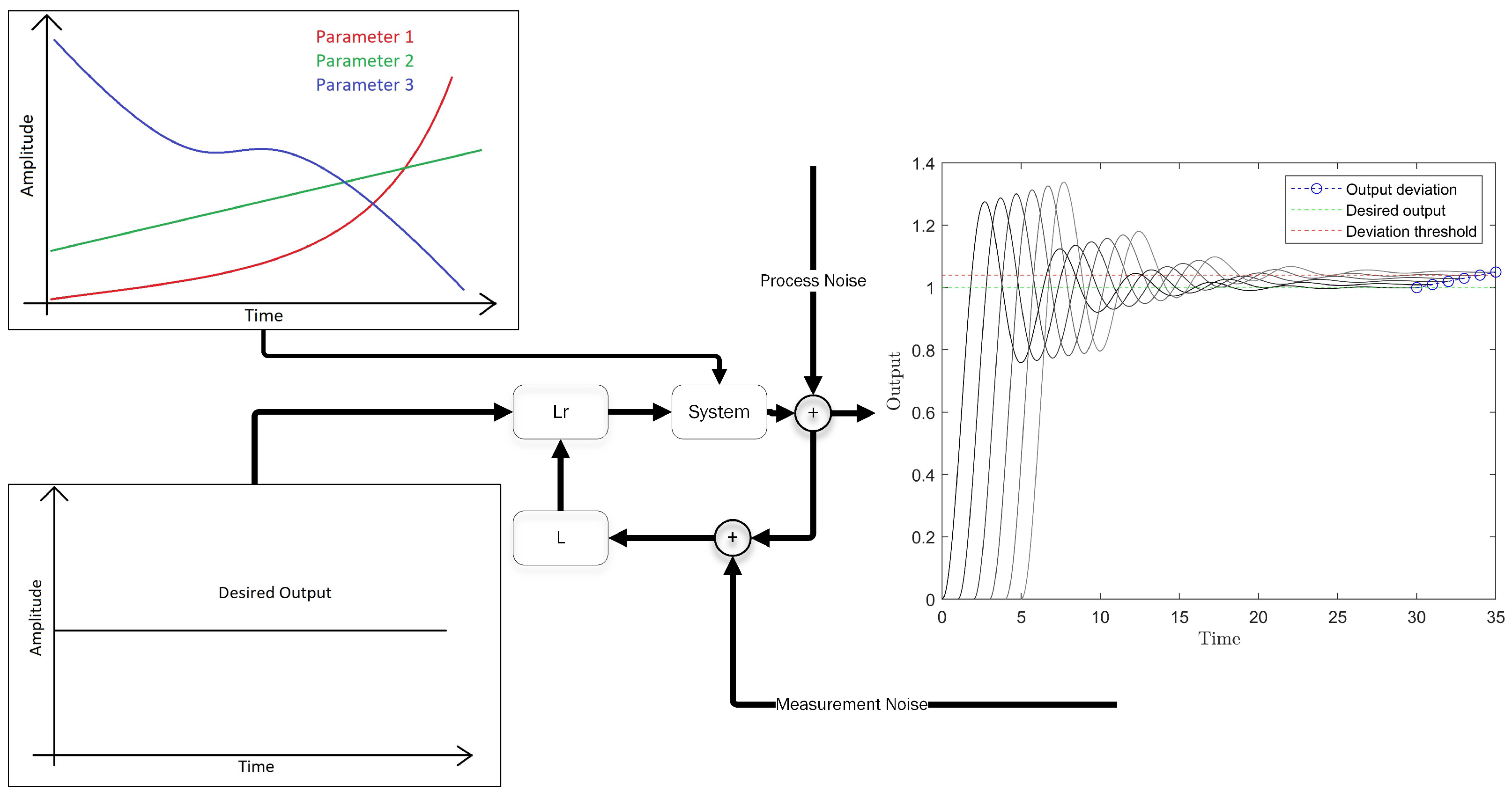
Figure 2.
Generation of the feature vector.

Figure 3.
Proposed method flowchart.
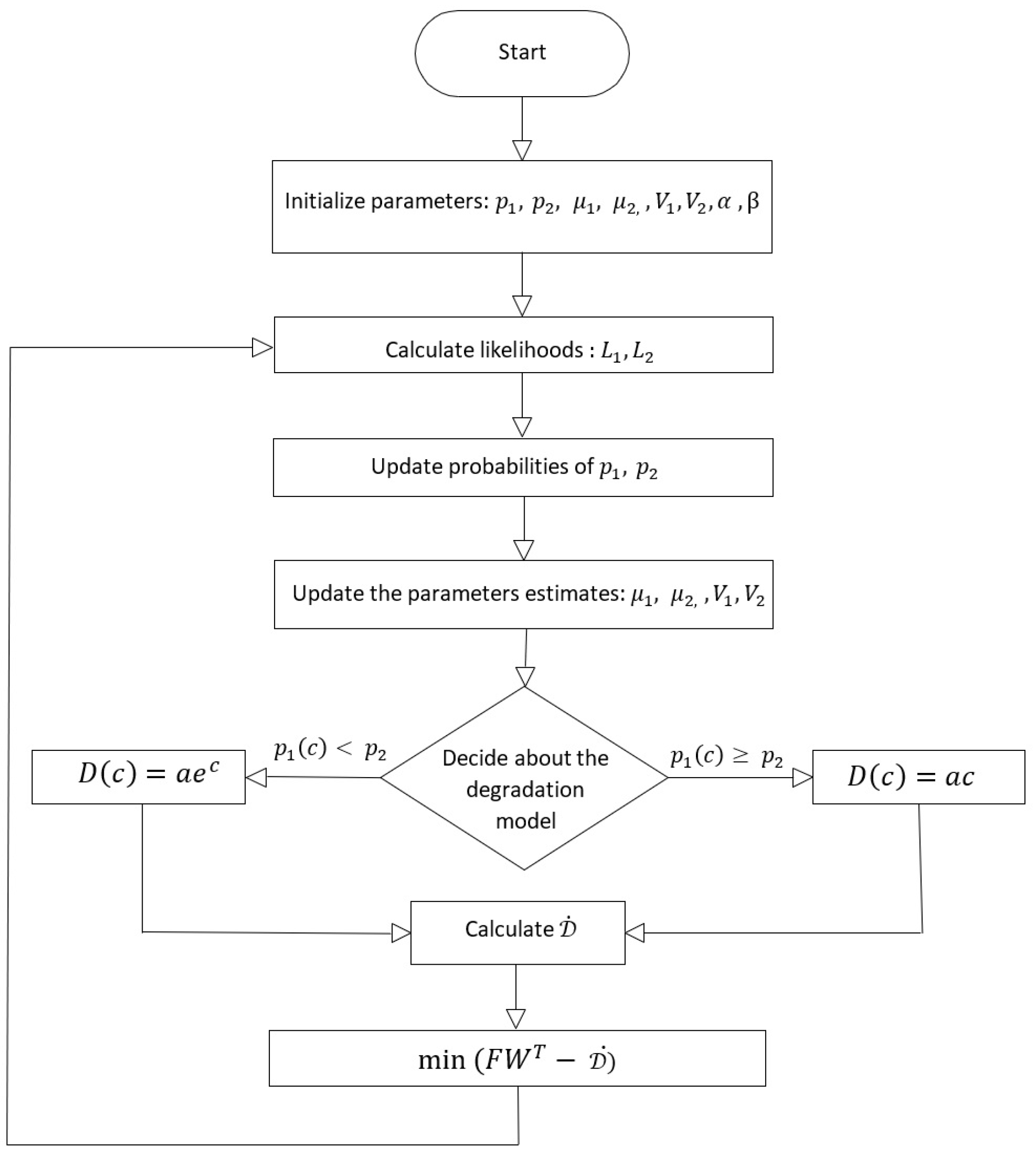
Figure 4.
Schematic of the rolling stand [50].
Figure 4.
Schematic of the rolling stand [50].

Figure 5.
Step response of the closed-loop system (two bottom plots in both figures are in log scale). (A) Closed-loop LQR response. (B) Closed-loop MPC response.
Figure 5.
Step response of the closed-loop system (two bottom plots in both figures are in log scale). (A) Closed-loop LQR response. (B) Closed-loop MPC response.
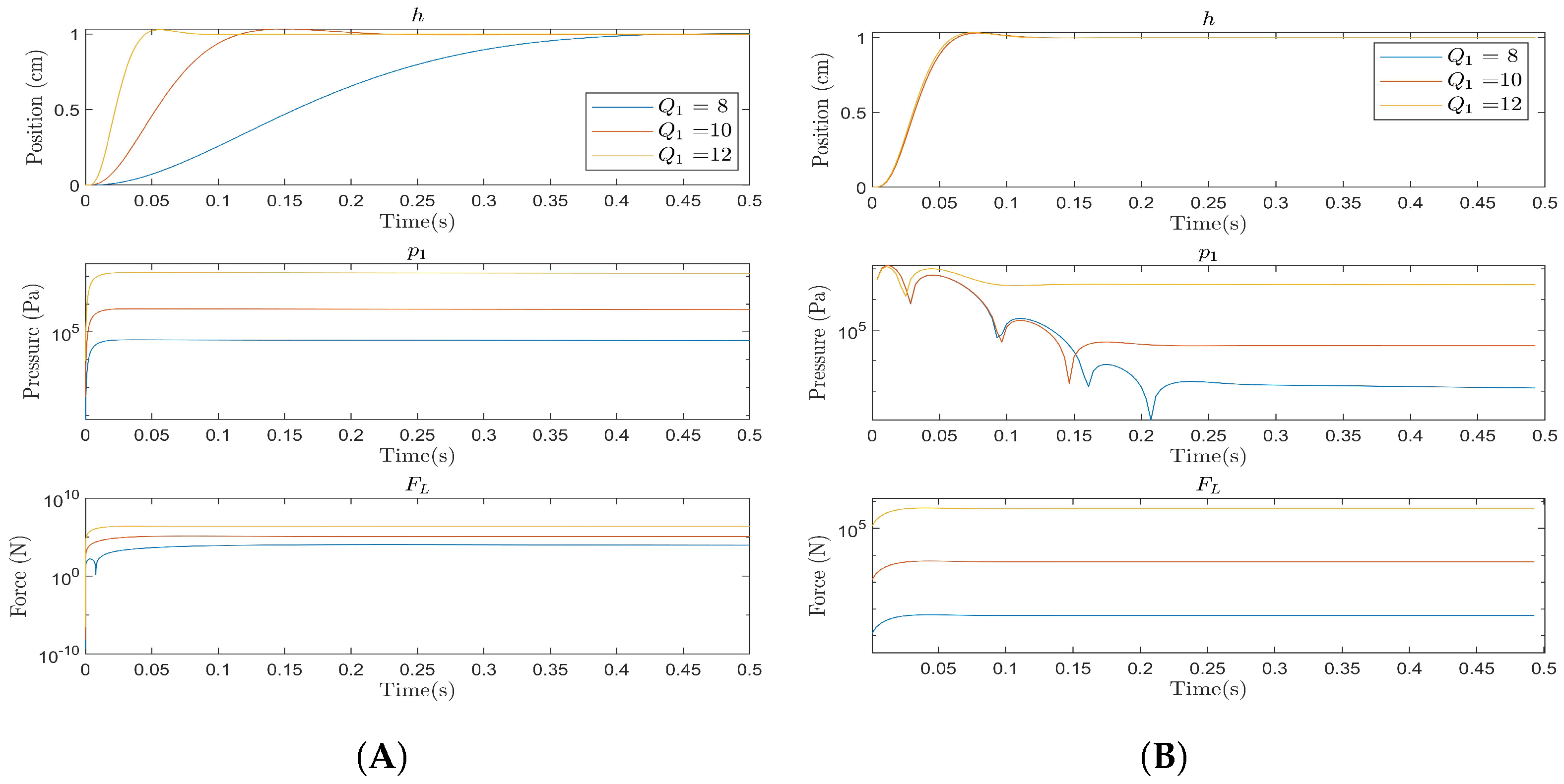
Figure 6.
Lifespan vs. penalty value. (A) 1st model—LQR. (B) 2nd model—LQR. (C) 3rd model—LQR. (D) 1st model—MPC. (E) 2nd model—MPC. (F) 3rd model—MPC.
Figure 6.
Lifespan vs. penalty value. (A) 1st model—LQR. (B) 2nd model—LQR. (C) 3rd model—LQR. (D) 1st model—MPC. (E) 2nd model—MPC. (F) 3rd model—MPC.

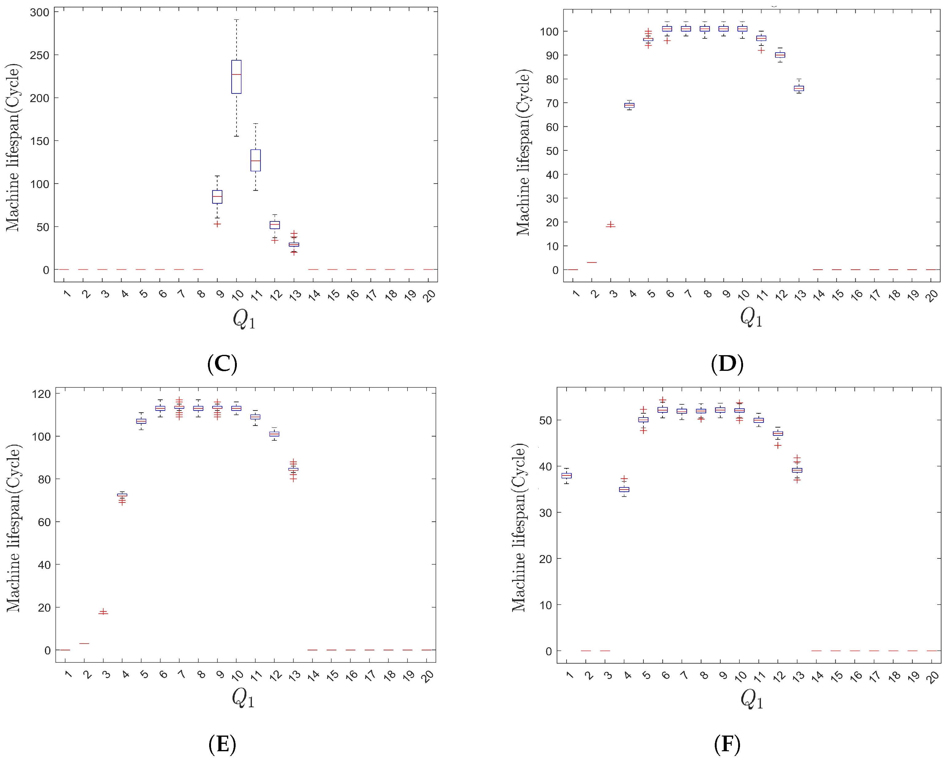
Figure 7.
Degradation in the closed-loop system using different controllers, . (A) Degradations in a closed-loop system using LQR. (B) Degradations in a closed-loop system using MPC.
Figure 7.
Degradation in the closed-loop system using different controllers, . (A) Degradations in a closed-loop system using LQR. (B) Degradations in a closed-loop system using MPC.
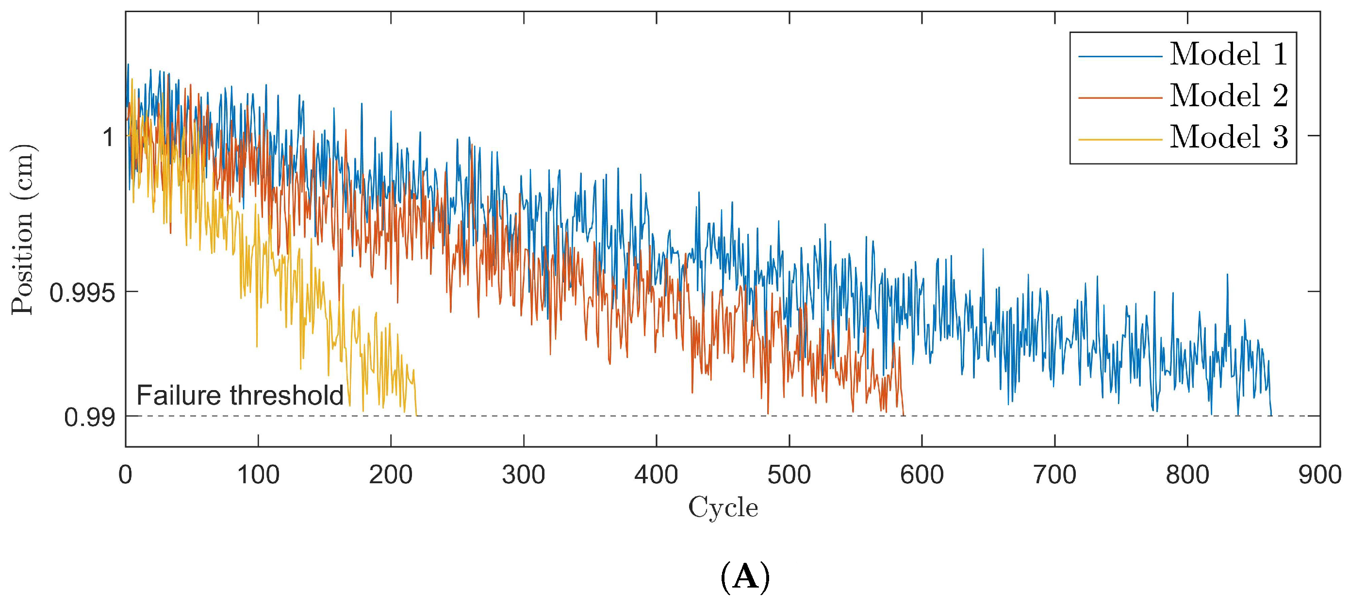
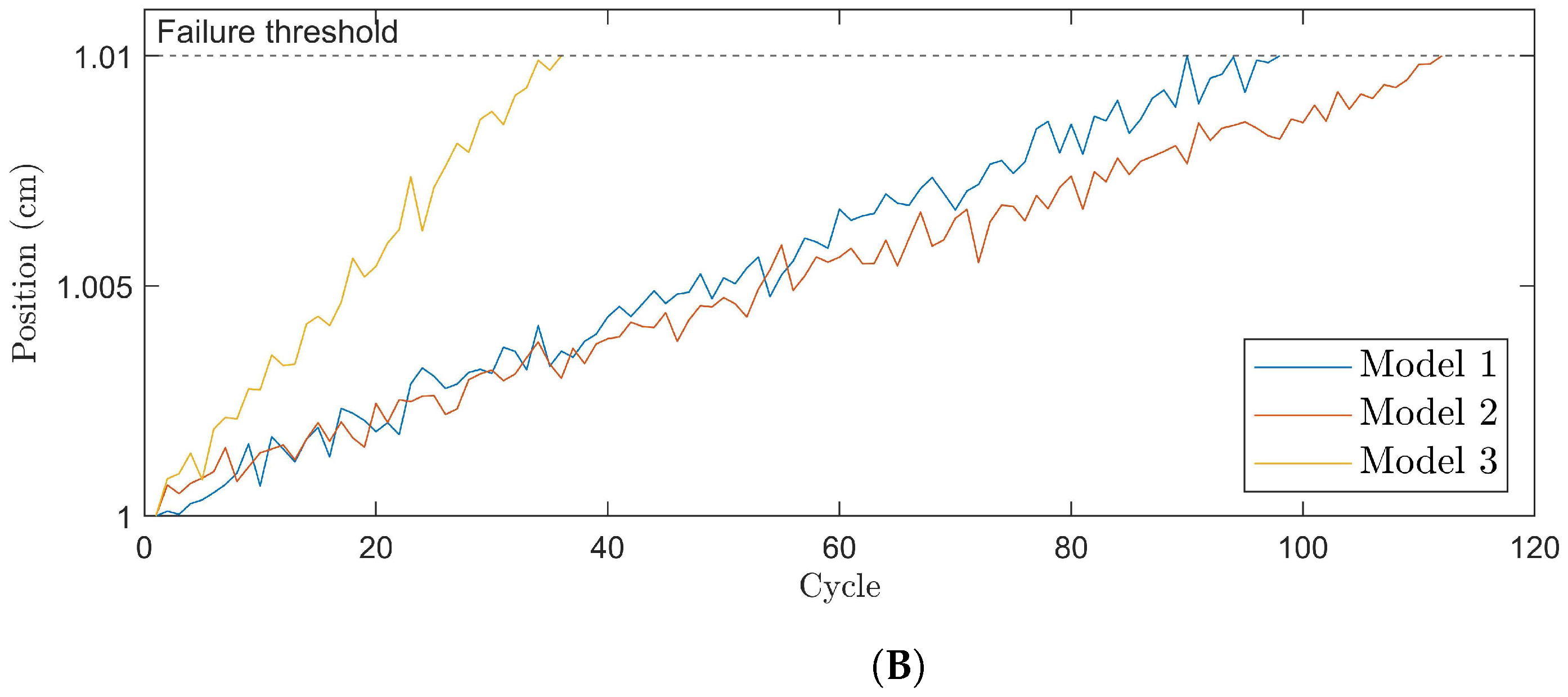
Figure 8.
Online calculation of the degradation coefficient for input force. (A) Degradation effect of , and with LQR. (B) Degradation effect of , and with MPC.
Figure 8.
Online calculation of the degradation coefficient for input force. (A) Degradation effect of , and with LQR. (B) Degradation effect of , and with MPC.
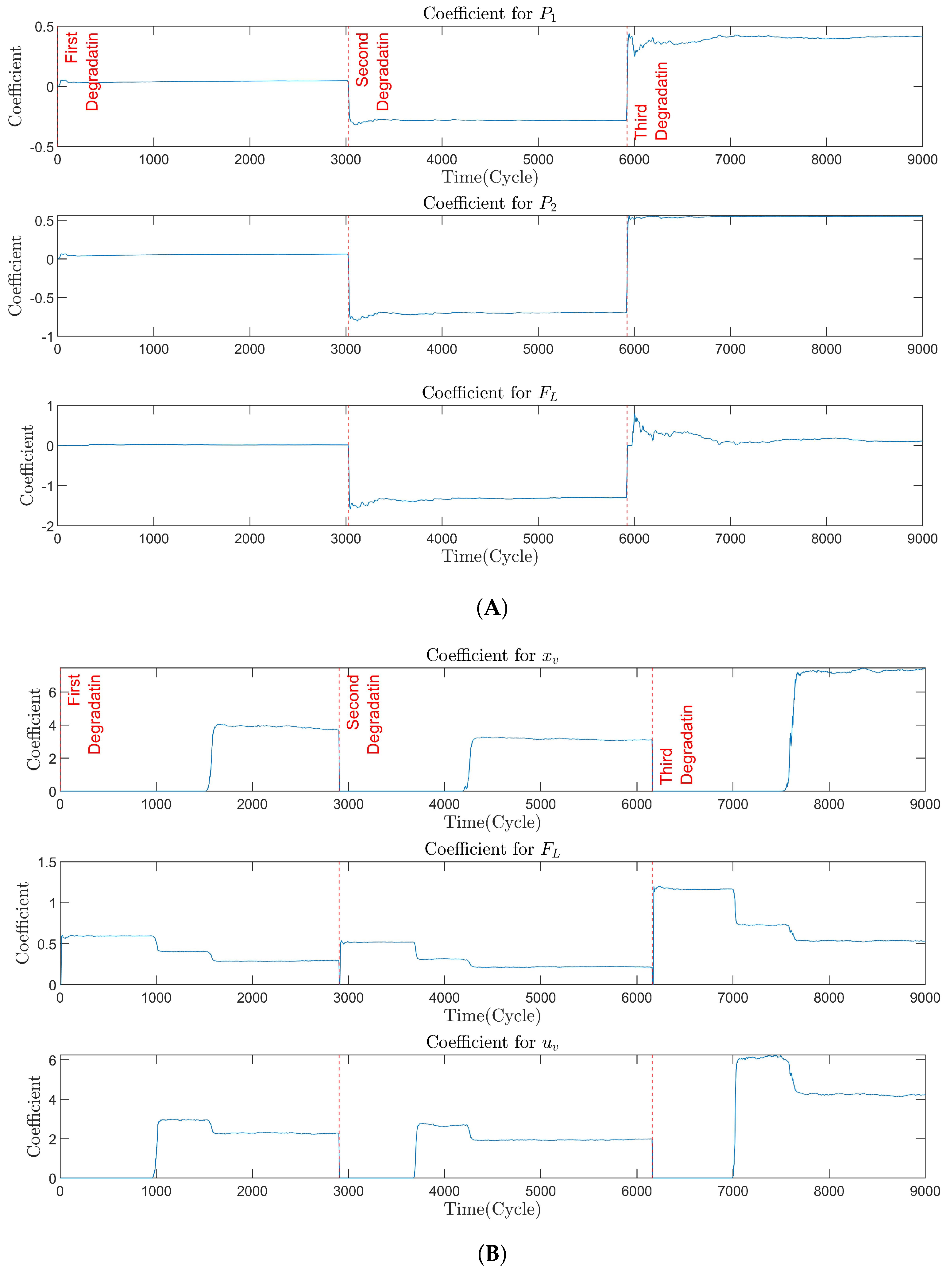
Figure 9.
Degradation-controlled system output. (A) LQR response to 1st degradation model. (B) MPC response to 1st degradation model. (C) LQR response to 2nd degradation model. (D) MPC response to 2nd degradation model. (E) LQR response to 3rd degradation model. (F) MPC response to 3rd degradation model.

Figure 10.
Step response using LQR degradation controller. (A) Without degradation control. (B) 1st degradation model. (C) 2nd degradation model.
Figure 10.
Step response using LQR degradation controller. (A) Without degradation control. (B) 1st degradation model. (C) 2nd degradation model.

Figure 11.
Lifespan vs. penalty values. (A) 1st model—LQR. (B) 2nd model—LQR. (C) 3rd model—LQR. (D) 1st model—MPC. (E) 2nd model—MPC. (F) 3rd model—MPC.
Figure 11.
Lifespan vs. penalty values. (A) 1st model—LQR. (B) 2nd model—LQR. (C) 3rd model—LQR. (D) 1st model—MPC. (E) 2nd model—MPC. (F) 3rd model—MPC.

Figure 12.
Control quality comparison, normal controller vs. degradation controller. (A) LQR controller quality. (B) MPC controller quality.
Figure 12.
Control quality comparison, normal controller vs. degradation controller. (A) LQR controller quality. (B) MPC controller quality.

Table 1.
Parameters used for the simulation.
| Parameter | Value | Unit |
|---|---|---|
| 0.1 | m | |
| 0.5 | m | |
| 0.65 | m | |
| Pa | ||
| 10 | N | |
| M | 100 | Kg |
| 10 | N | |
| Pa | ||
| 900 | ||
| 0.001 | s | |
| - | ||
| - | ||
| 1 | - |
Table 2.
Degradation models’ parameters.
| Parameter | Model 1 | Model 2 | Model 3 |
|---|---|---|---|
| 0 | |||
| 0 | 0 | ||
Table 3.
Degradation coefficients calculated using RVM.
| Par. | Effect on Degradation | |||||
|---|---|---|---|---|---|---|
| LQR | MPC | |||||
| Deg. 1 | Deg. 2 | Deg. 3 | Deg. 1 | Deg. 2 | Deg. 3 | |
| h | 0 | 0 | 0 | 0 | 0 | 0 |
| 0 | 0 | 0 | 0 | 0 | 0 | |
| 0.04 | −0.28 | 0.40 | 0 | 0 | 0 | |
| 0.06 | −0.69 | 0.55 | 0 | 0 | 0 | |
| 0 | 0 | 0 | 3.73 | 3.12 | 7.39 | |
| 0.01 | −1.29 | 0.12 | 0.29 | 0.21 | 0.53 | |
| 0 | 0 | 0 | 2.29 | 1.99 | 4.20 | |
Disclaimer/Publisher’s Note: The statements, opinions and data contained in all publications are solely those of the individual author(s) and contributor(s) and not of MDPI and/or the editor(s). MDPI and/or the editor(s) disclaim responsibility for any injury to people or property resulting from any ideas, methods, instructions or products referred to in the content. |
© 2023 by the authors. Licensee MDPI, Basel, Switzerland. This article is an open access article distributed under the terms and conditions of the Creative Commons Attribution (CC BY) license (https://creativecommons.org/licenses/by/4.0/).
Share and Cite
MDPI and ACS Style
Dadash, A.H.; Björsell, N. Optimal Degradation-Aware Control Using Process-Controlled Sparse Bayesian Learning. Processes 2023, 11, 3229. https://doi.org/10.3390/pr11113229
AMA Style
Dadash AH, Björsell N. Optimal Degradation-Aware Control Using Process-Controlled Sparse Bayesian Learning. Processes. 2023; 11(11):3229. https://doi.org/10.3390/pr11113229
Chicago/Turabian StyleDadash, Amirhossein Hosseinzadeh, and Niclas Björsell. 2023. "Optimal Degradation-Aware Control Using Process-Controlled Sparse Bayesian Learning" Processes 11, no. 11: 3229. https://doi.org/10.3390/pr11113229
Note that from the first issue of 2016, this journal uses article numbers instead of page numbers. See further details here.