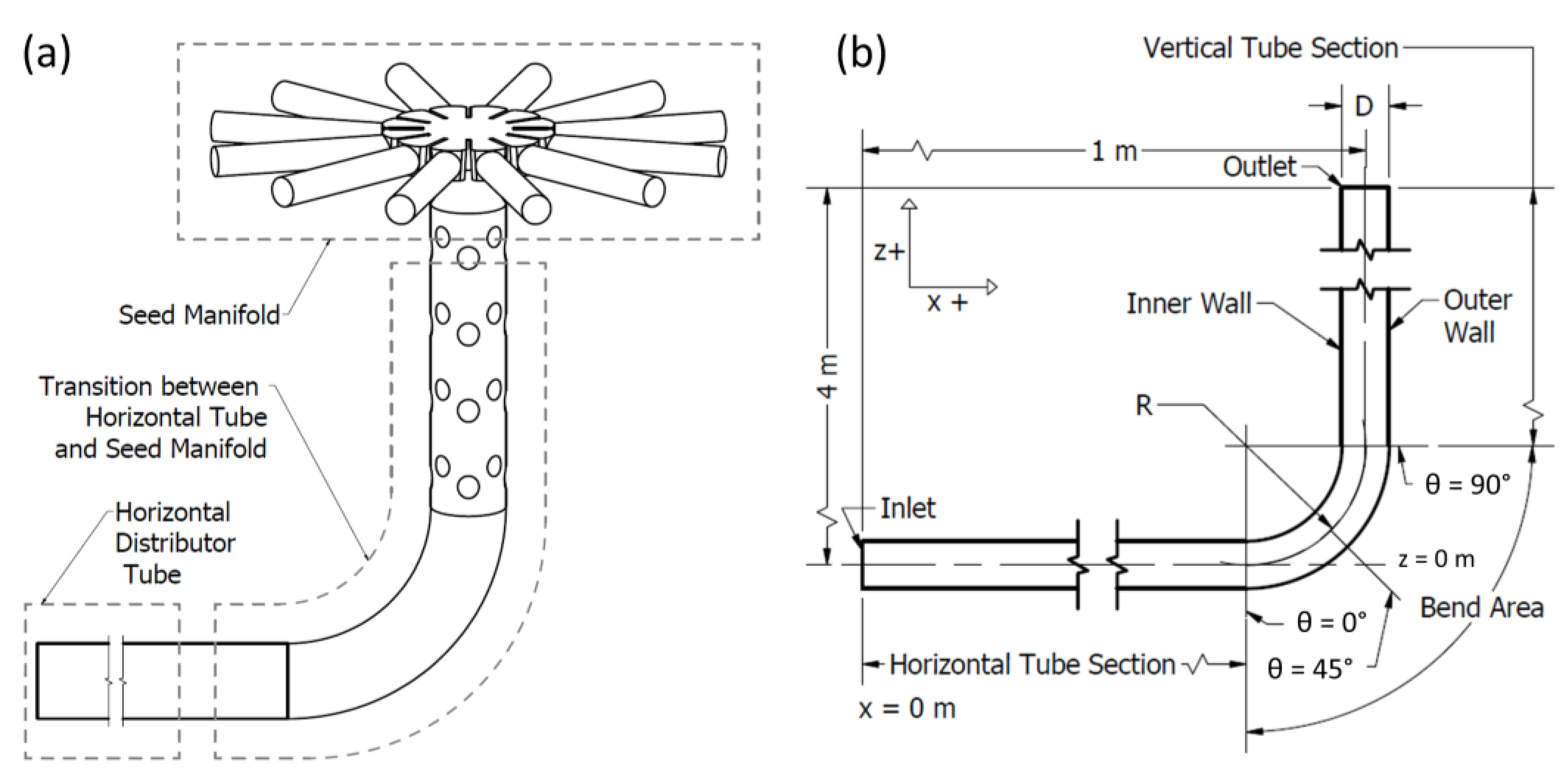
Figure 1.
Horizontal-vertical 90-degree elbow transition: (a) typical air seeder system, and (b) simulation geometry.
Figure 1.
Horizontal-vertical 90-degree elbow transition: (a) typical air seeder system, and (b) simulation geometry.
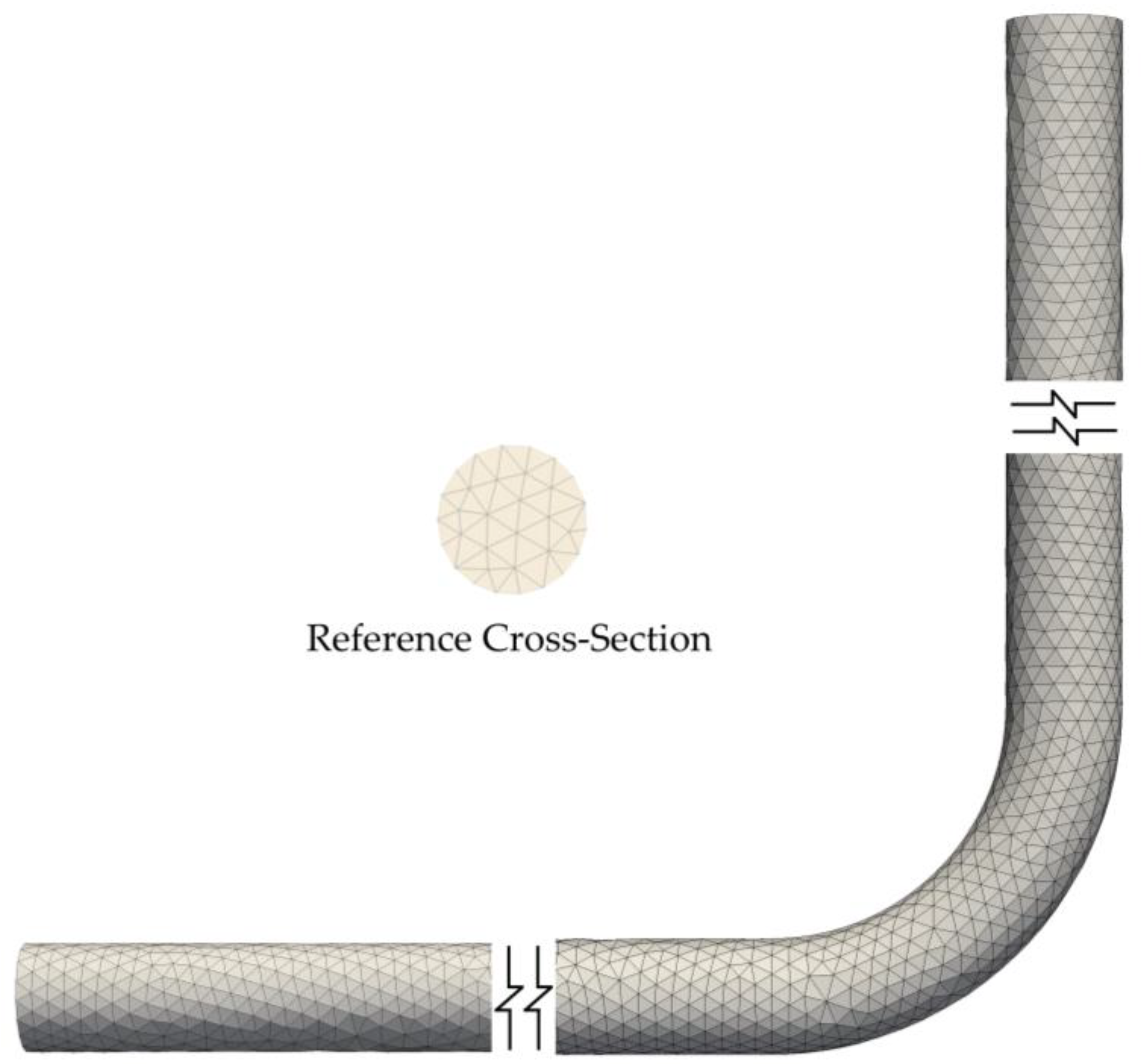
Figure 2.
Sample computational fluid dynamics (CFD) mesh views: horizontal-vertical 90-degree elbow for simulation sets 1 and 2.
Figure 2.
Sample computational fluid dynamics (CFD) mesh views: horizontal-vertical 90-degree elbow for simulation sets 1 and 2.
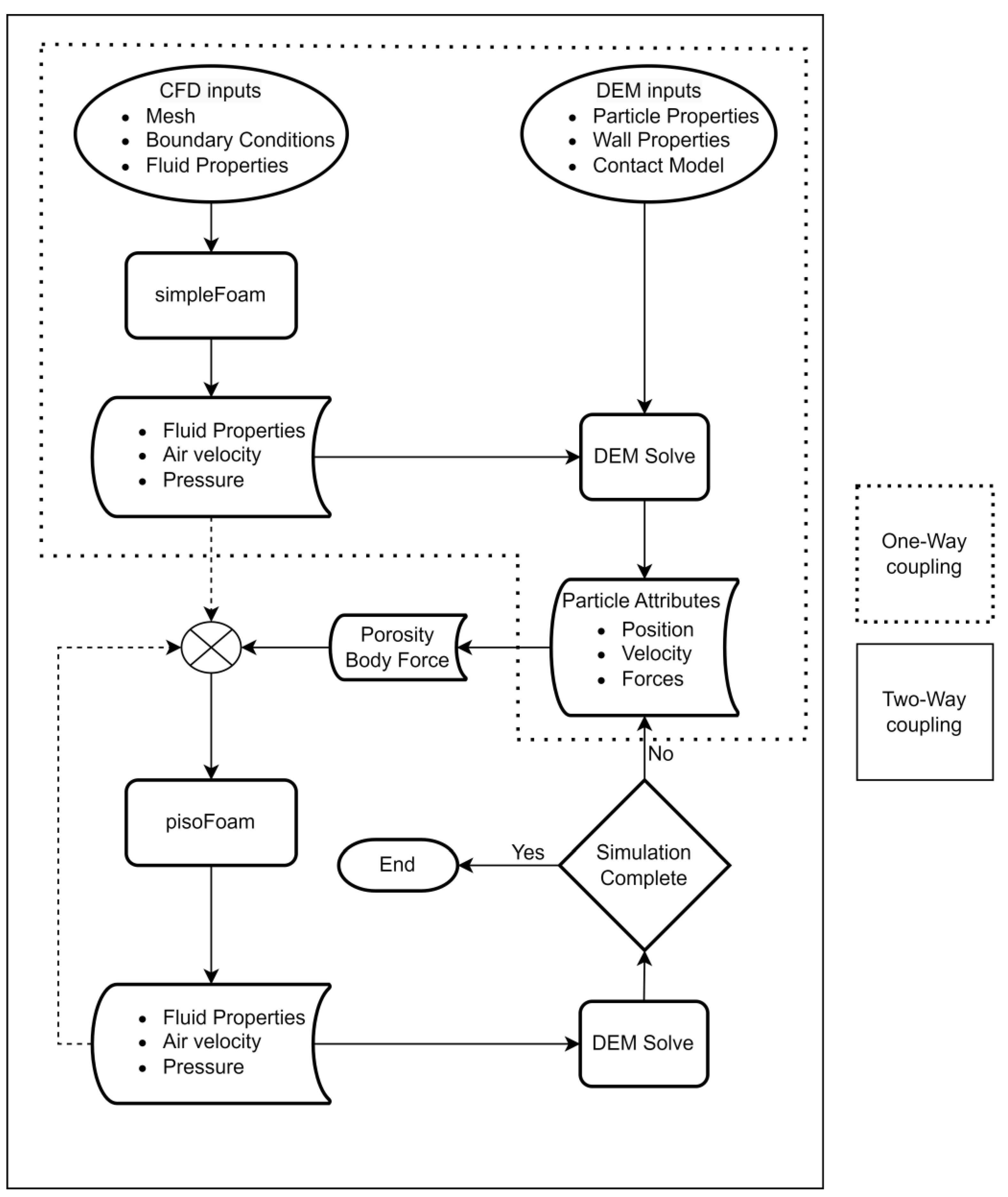
Figure 3.
Reference diagram for one-way and two-way CFD-DEM coupling process.
Figure 3.
Reference diagram for one-way and two-way CFD-DEM coupling process.
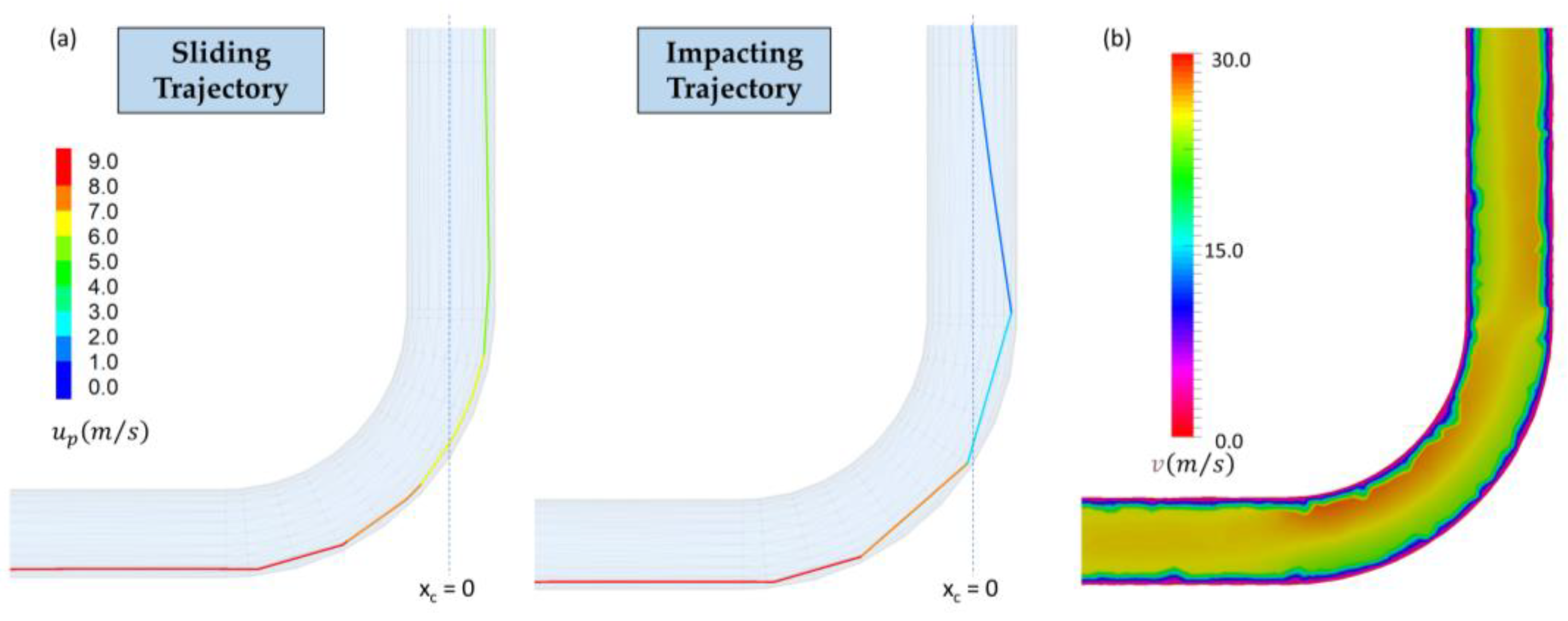
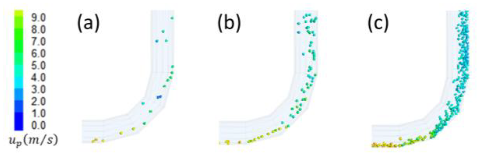
Figure 4.
Simulated seed trajectory at a horizontal-vertical 90-degree elbow for 0.070 kg/s seed rate and air velocity (v) of 25 m/s: (a) seed path (up = Particle velocity, xc = horizontal seed position relative to tube centerline), (b) sample airflow velocity profile.
Figure 4.
Simulated seed trajectory at a horizontal-vertical 90-degree elbow for 0.070 kg/s seed rate and air velocity (v) of 25 m/s: (a) seed path (up = Particle velocity, xc = horizontal seed position relative to tube centerline), (b) sample airflow velocity profile.
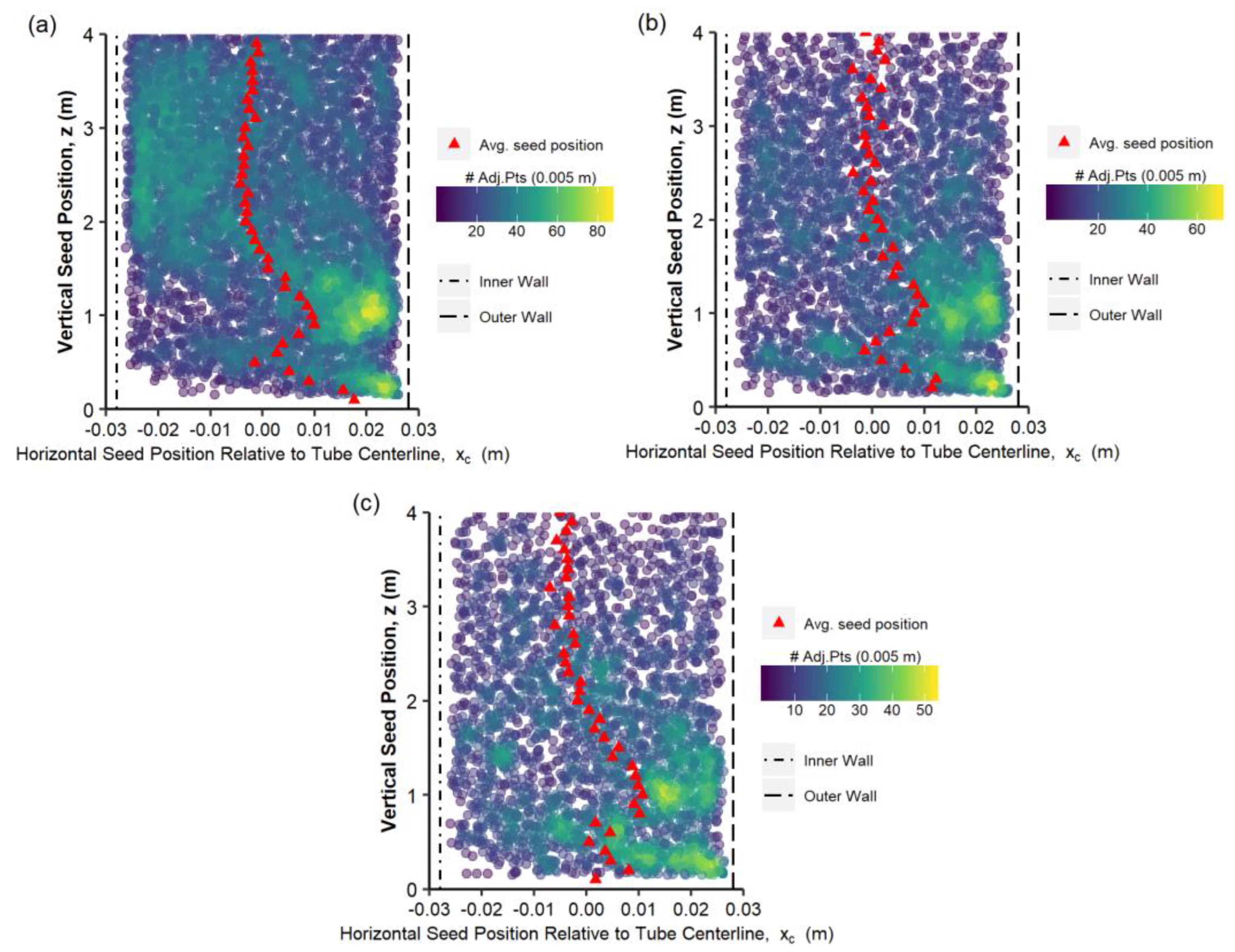
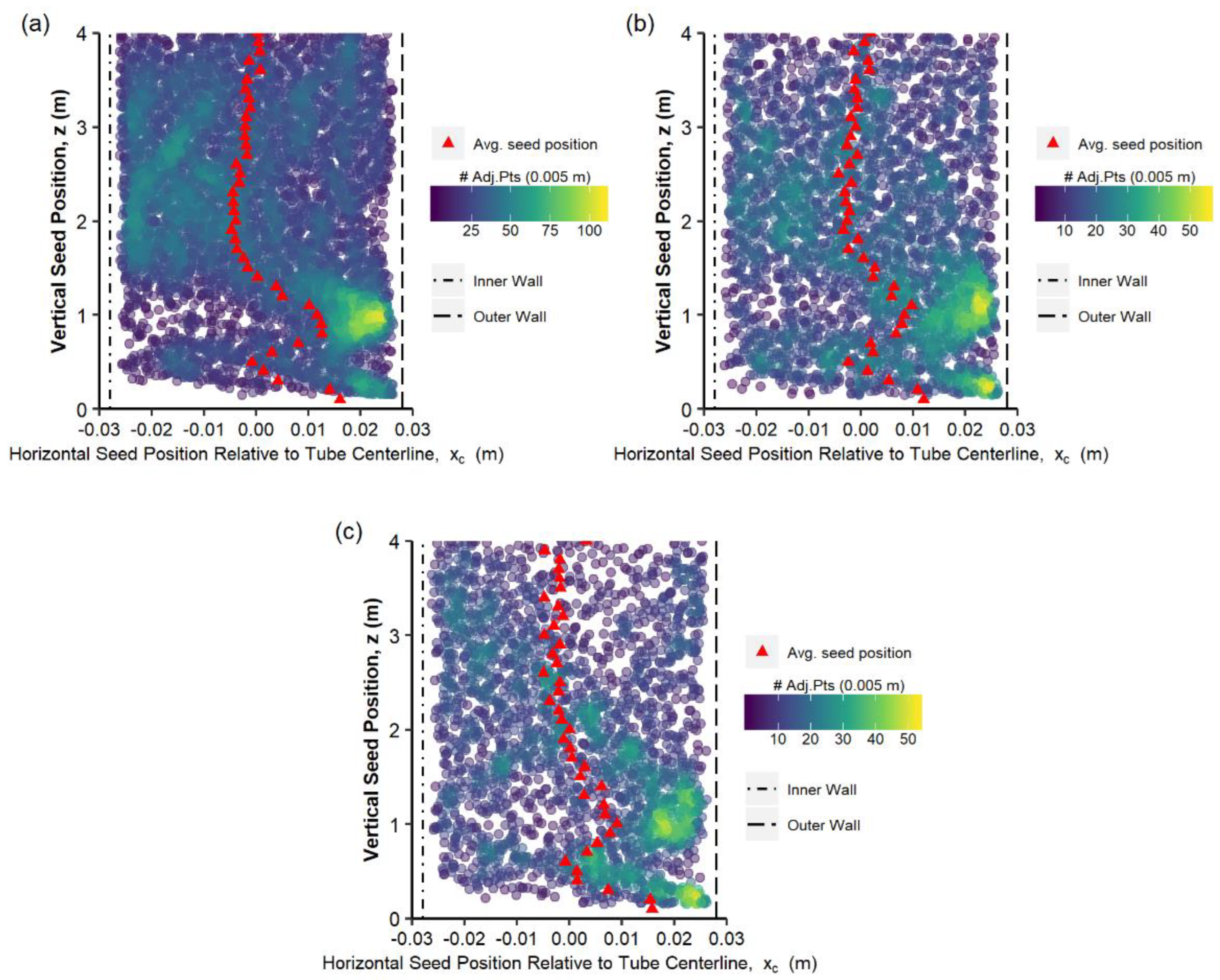
Figure 5.
One-way coupled seed trajectory density plot, number (#) of adjacent points, and average seed positions for a seed rate of 0.070 kg/s and air velocities of (a) 20 m/s, (b) 25 m/s and (c) 30 m/s.
Figure 5.
One-way coupled seed trajectory density plot, number (#) of adjacent points, and average seed positions for a seed rate of 0.070 kg/s and air velocities of (a) 20 m/s, (b) 25 m/s and (c) 30 m/s.
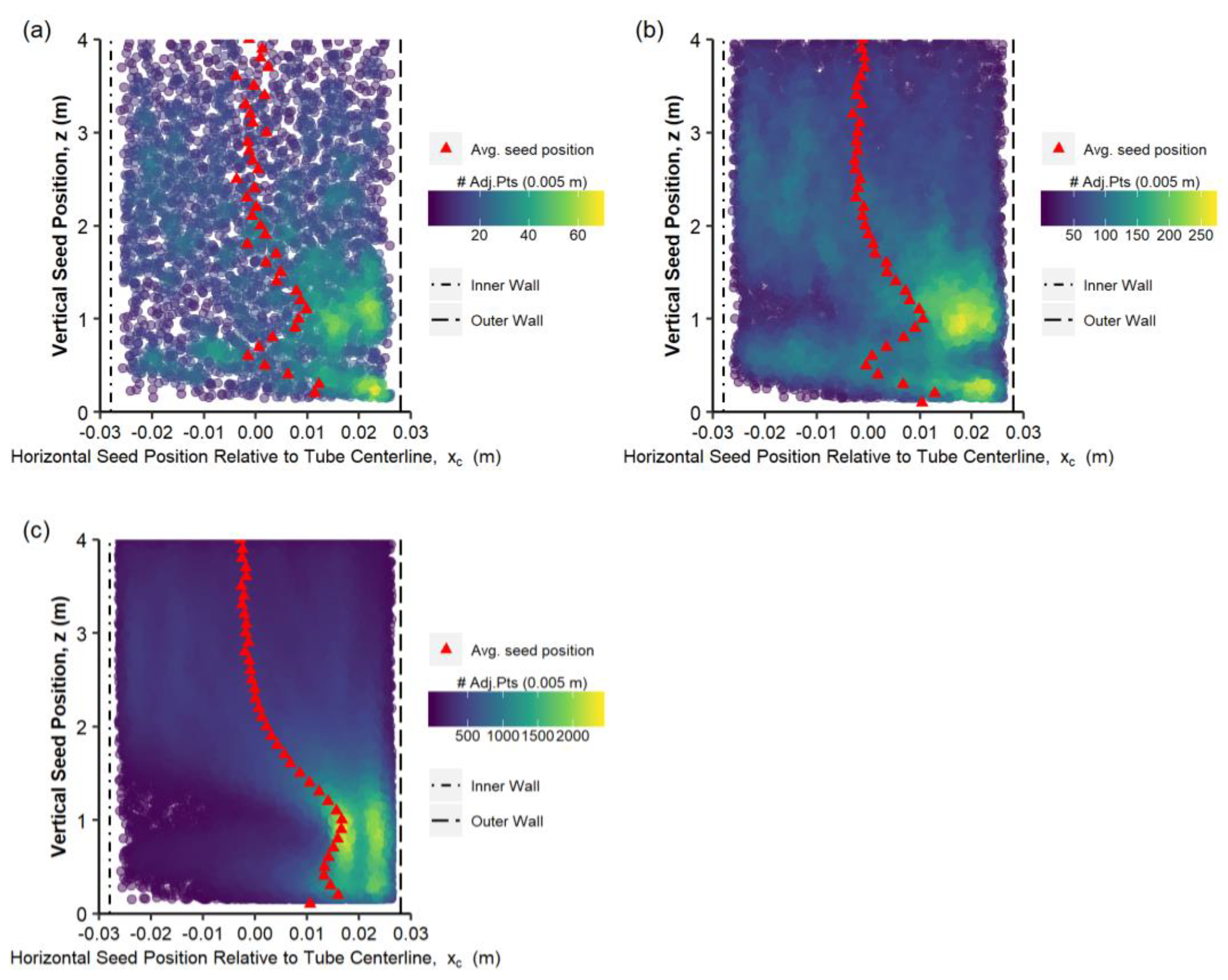
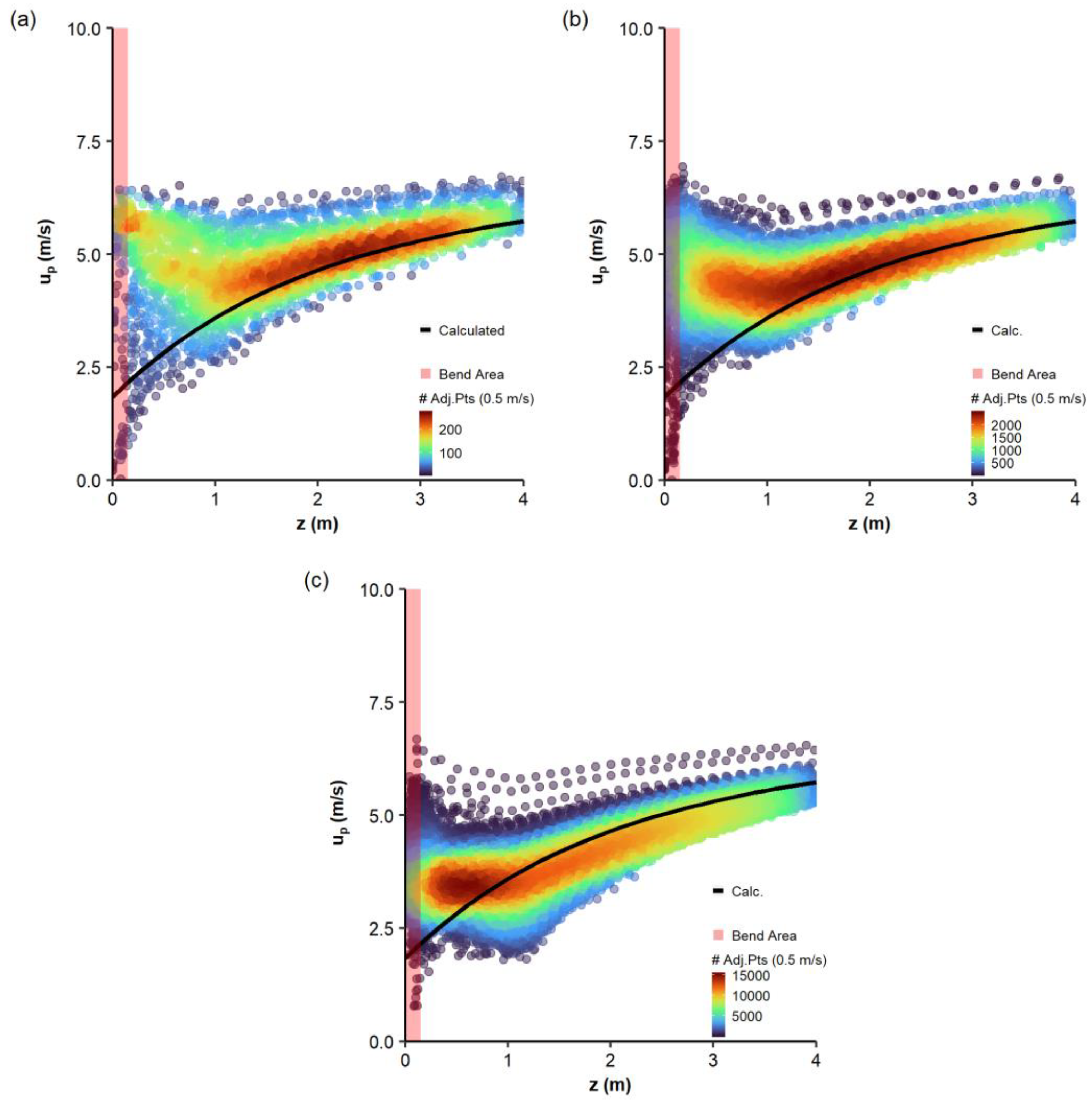
Figure 6.
Seed trajectory density plot, number (#) of adjacent points, and average seed positions for 25 m/s air velocity and seed rates of (a) 0.07 kg/s, (b) 0.21 Kg/s and (c) 0.42 kg/s.
Figure 6.
Seed trajectory density plot, number (#) of adjacent points, and average seed positions for 25 m/s air velocity and seed rates of (a) 0.07 kg/s, (b) 0.21 Kg/s and (c) 0.42 kg/s.
Figure 7.
One-way coupled seed trajectory in horizontal-vertical 90-degree elbow for air velocity of 25 m/s and seed rates of (a) 0.07 kg/s, (b) 0.21 kg/s and (c) 0.42 kg/s.
Figure 7.
One-way coupled seed trajectory in horizontal-vertical 90-degree elbow for air velocity of 25 m/s and seed rates of (a) 0.07 kg/s, (b) 0.21 kg/s and (c) 0.42 kg/s.
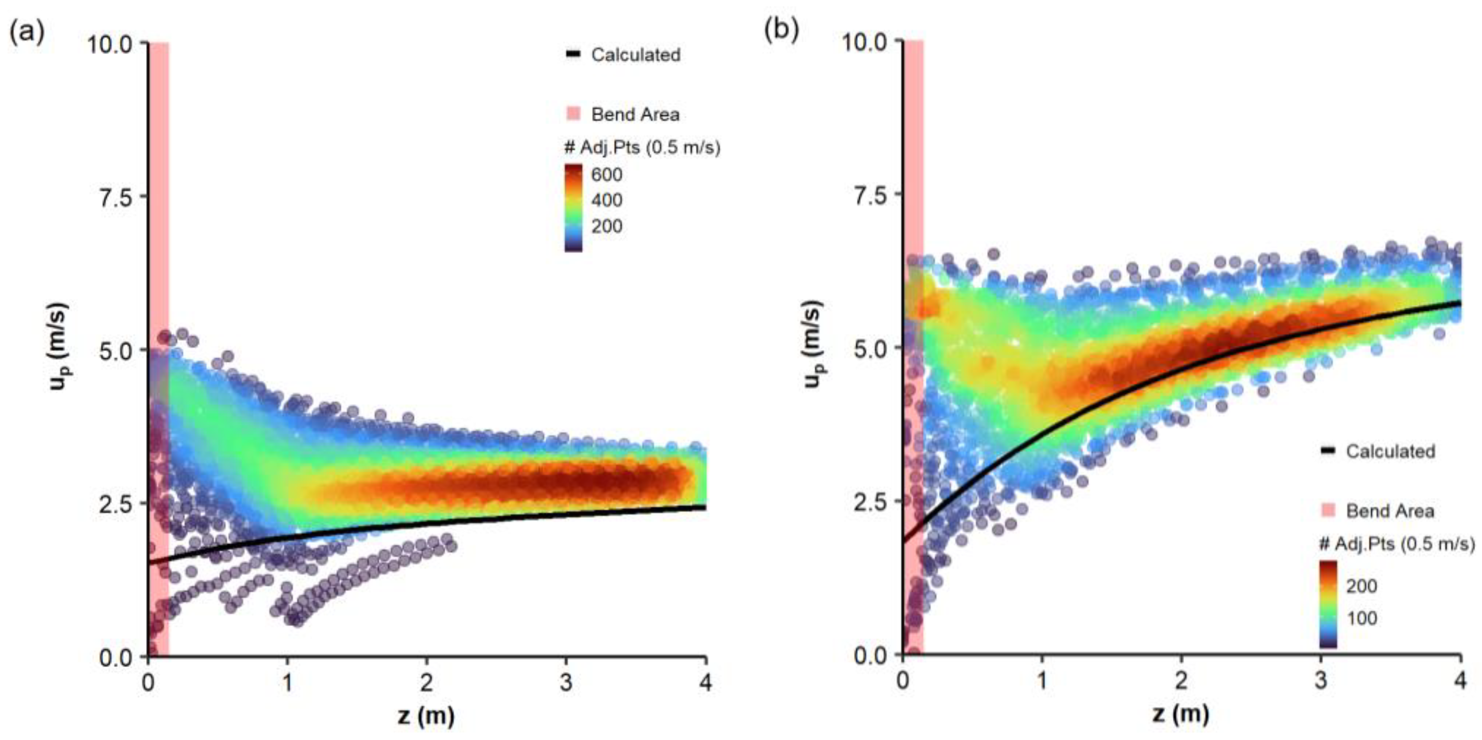
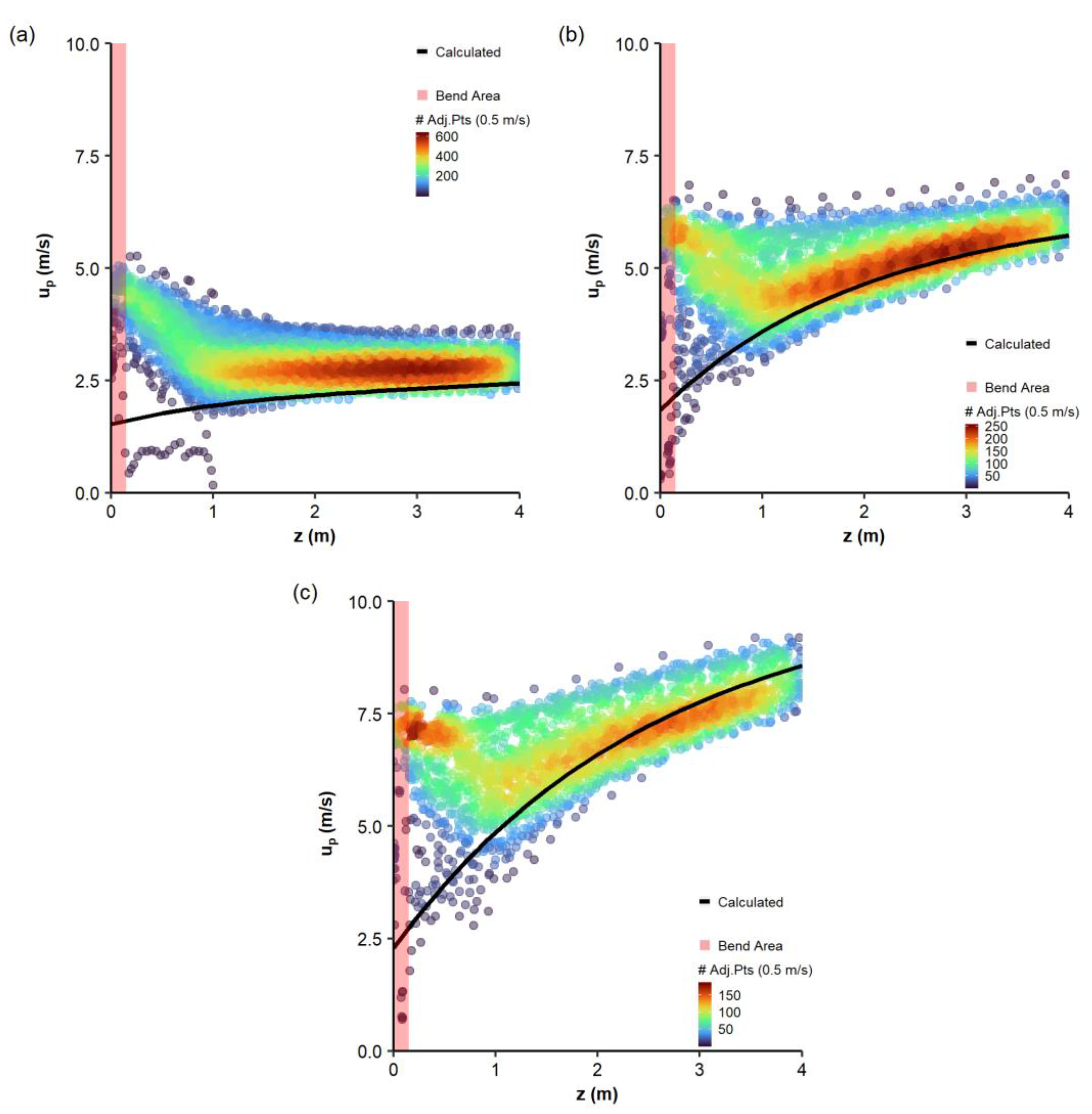
Figure 8.
One-way coupled simulation density plot, number (#) of adjacent points, data for seed velocities (up) along the vertical tube section (z) at seed rate of 0.07 kg/s and air velocities of (a) 20 m/s, (b) 25 m/s, and (c) 30 m/s.
Figure 8.
One-way coupled simulation density plot, number (#) of adjacent points, data for seed velocities (up) along the vertical tube section (z) at seed rate of 0.07 kg/s and air velocities of (a) 20 m/s, (b) 25 m/s, and (c) 30 m/s.
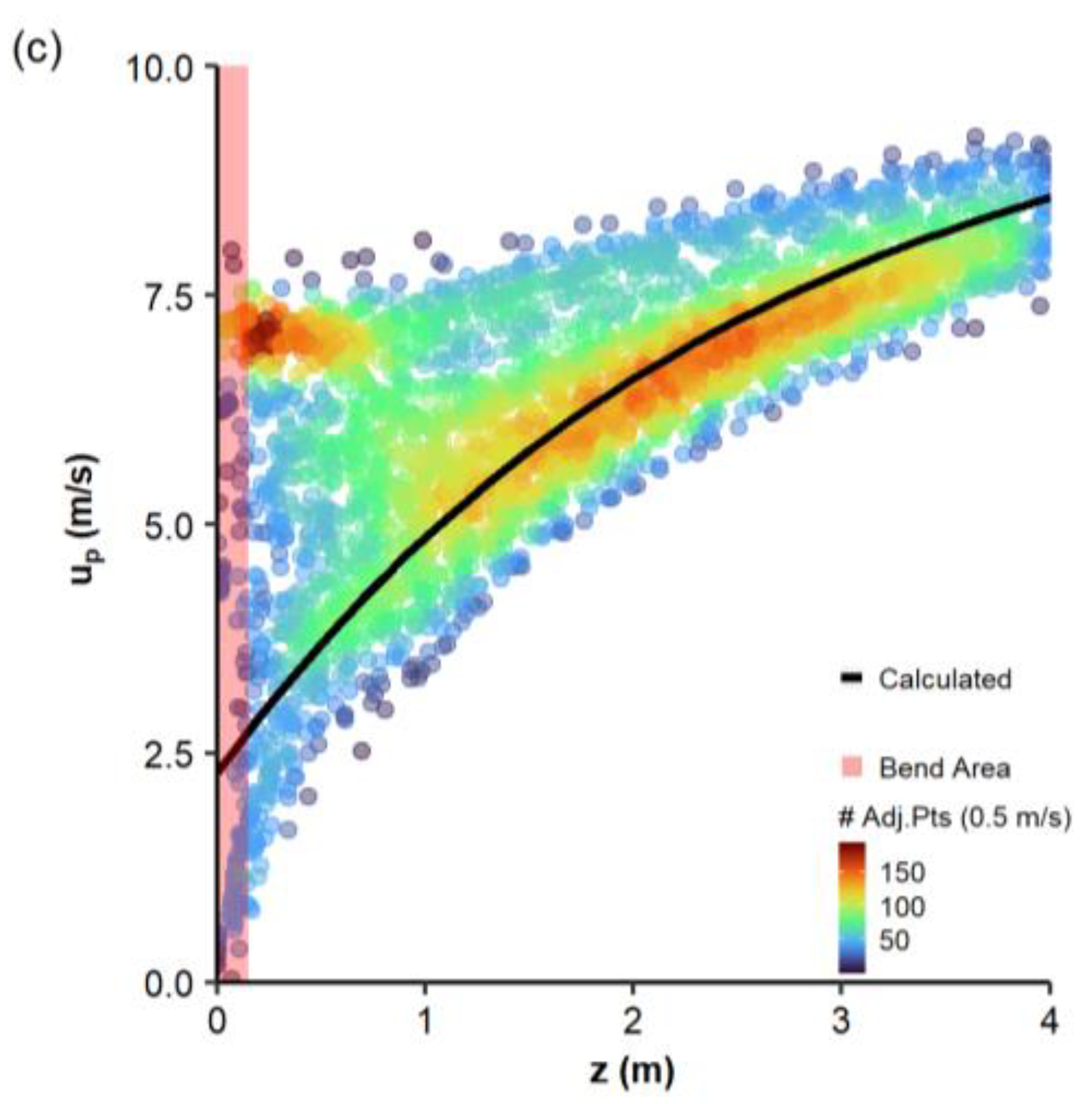
Figure 9.
One-way coupled simulation density plot, number (#) of adjacent points, data for seed velocities (up) in horizontal-vertical 90-degree elbow along the vertical tube section (z) at air velocity of 25 m/s and seed rate of (a) 0.07 kg/s, (b) 0.21 kg/s, and (c) 0.42 kg/s.
Figure 9.
One-way coupled simulation density plot, number (#) of adjacent points, data for seed velocities (up) in horizontal-vertical 90-degree elbow along the vertical tube section (z) at air velocity of 25 m/s and seed rate of (a) 0.07 kg/s, (b) 0.21 kg/s, and (c) 0.42 kg/s.
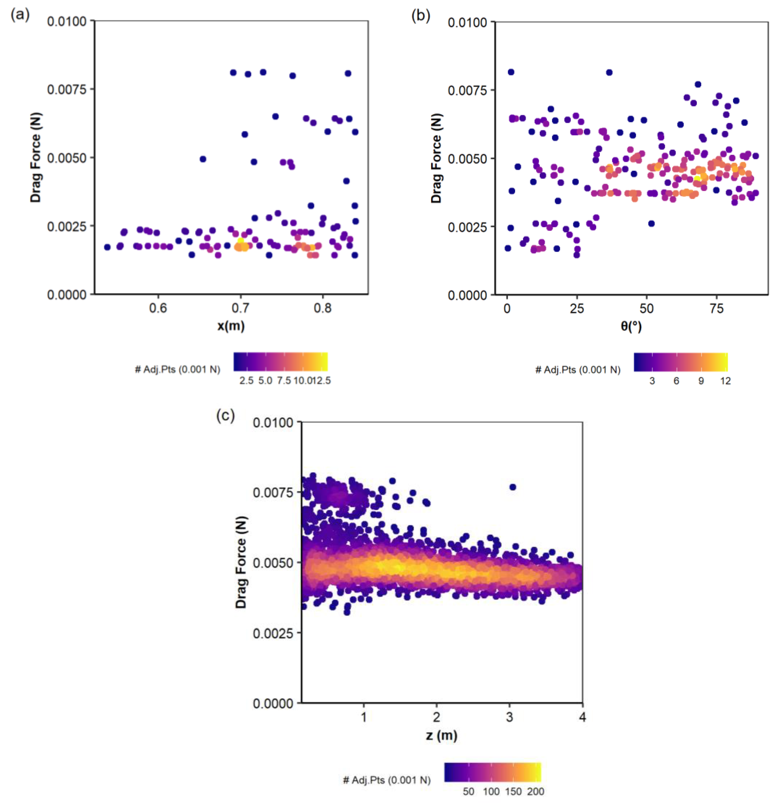
Figure 10.
One-way coupled simulation density plot, number (#) of adjacent points, data showing seed drag force for air velocity of 25 m/s and seed rate of 0.07 kg/s at different elbow locations: (a) horizontal tube section (x), (b) angle within bend area (θ), and (c) vertical tube section (z).
Figure 10.
One-way coupled simulation density plot, number (#) of adjacent points, data showing seed drag force for air velocity of 25 m/s and seed rate of 0.07 kg/s at different elbow locations: (a) horizontal tube section (x), (b) angle within bend area (θ), and (c) vertical tube section (z).
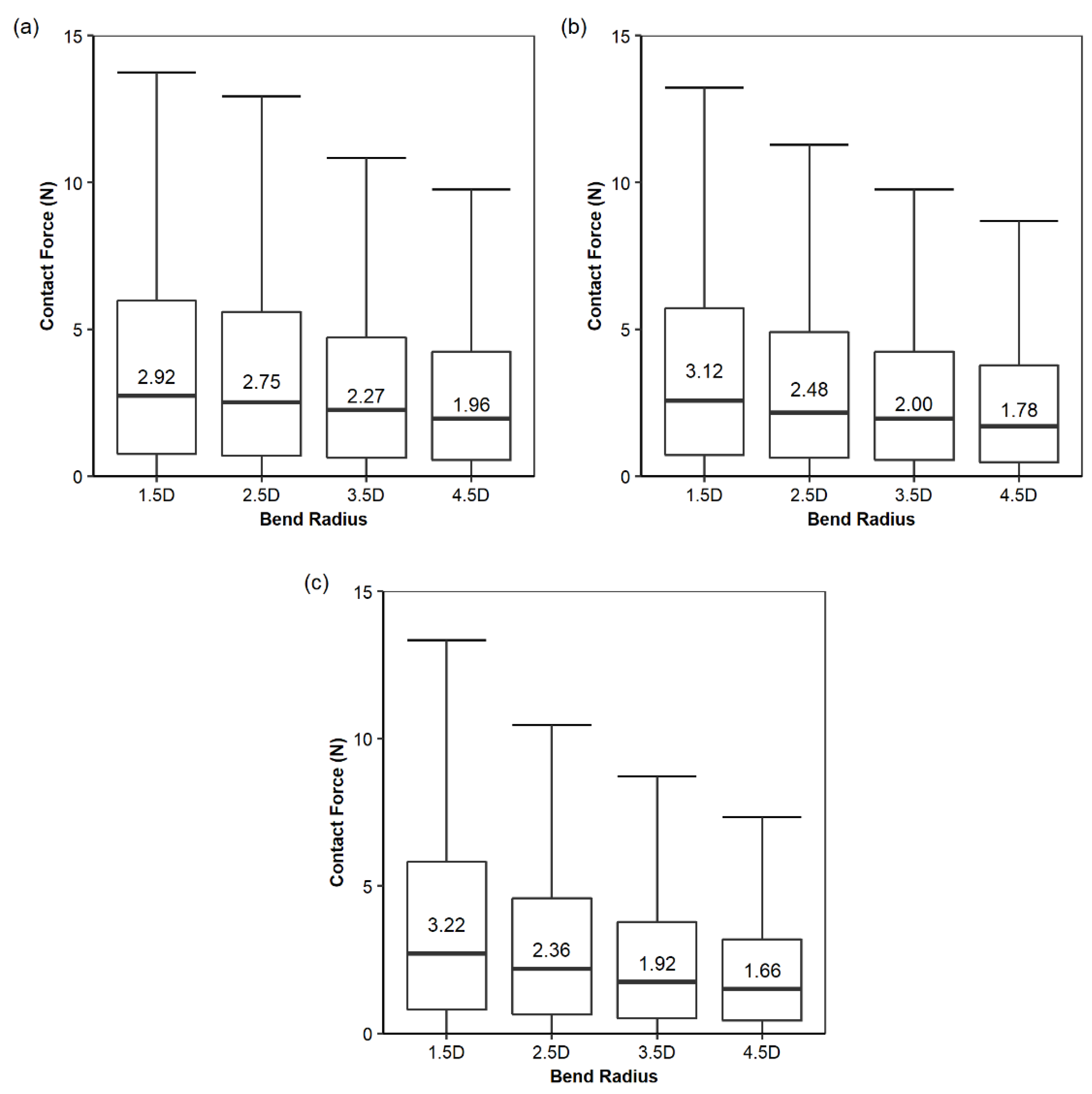
Figure 11.
Seed contact force box plots at the elbow area as a function of bend radius for different elbow diameters: (a) 48.3 mm, (b) 60.3 mm, (c) 72.4 mm.
Figure 11.
Seed contact force box plots at the elbow area as a function of bend radius for different elbow diameters: (a) 48.3 mm, (b) 60.3 mm, (c) 72.4 mm.
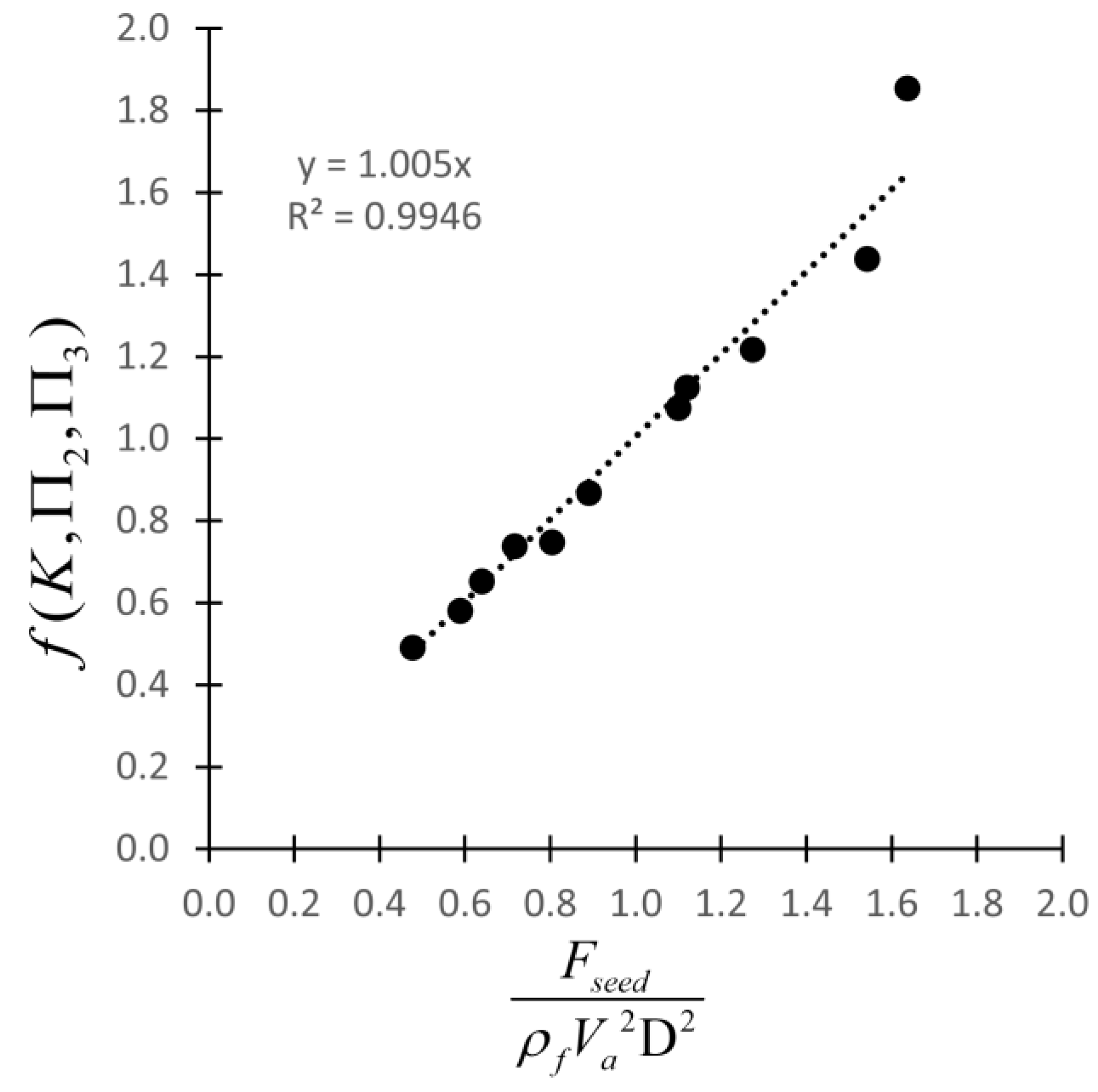
Figure 12.
Relationship between Pi groups and dimensionless seed contact force.
Figure 12.
Relationship between Pi groups and dimensionless seed contact force.
Figure 13.
Two-way coupled seed trajectory density plot, number (#) of adjacent points, and average seed positions for a seed rate of 0.07 kg/s and air velocities of (a) 20 m/s, (b) 25 m/s, and (c) 30 m/s.
Figure 13.
Two-way coupled seed trajectory density plot, number (#) of adjacent points, and average seed positions for a seed rate of 0.07 kg/s and air velocities of (a) 20 m/s, (b) 25 m/s, and (c) 30 m/s.
Figure 14.
Two-way CFD-DEM coupled simulation density plot, number (#) of adjacent points, data for seed velocities (up) along the vertical tube section (z) at seed rate of 0.07 kg/s and air velocities of (a) 20 m/s, (b) 25 m/s, and (c) 30 m/s.
Figure 14.
Two-way CFD-DEM coupled simulation density plot, number (#) of adjacent points, data for seed velocities (up) along the vertical tube section (z) at seed rate of 0.07 kg/s and air velocities of (a) 20 m/s, (b) 25 m/s, and (c) 30 m/s.
Figure 15.
Two-way coupled simulation density plot, number (#) of adjacent points, data showing seed drag force for air velocity of 25 m/s and seed rate of 0.07 kg/s at different elbow locations: (a) horizontal tube section (x), (b) angle within bend area (θ), and (c) vertical tube section (z).
Figure 15.
Two-way coupled simulation density plot, number (#) of adjacent points, data showing seed drag force for air velocity of 25 m/s and seed rate of 0.07 kg/s at different elbow locations: (a) horizontal tube section (x), (b) angle within bend area (θ), and (c) vertical tube section (z).
Table 1.
Discrete element method (DEM) input parameters.
Table 1.
Discrete element method (DEM) input parameters.
| Parameter | Symbol | Unit | Value | Reference |
|---|
| Particle Density, Pea Seed | ρp | kg/m3 | 1720 | [21] |
| Particle Diameter, Pea seed | d | mm | 6.94 | [23] |
| Modulus of Elasticity, Pea Seed | Ep | Pa | 236 × 106 | [20] |
| Shear Modulus, Pea Seed | Pg | Pa | 98.3 × 10⁶ | Calculated from Ep |
| Modulus of Elasticity, Wall | Ew | Pa | 200 × 109 | - |
| Shear Modulus, Wall | Gw | Pa | 76.8 × 10⁹ | Calculated from Ew |
| Poisson’s Ratio, Pea Seed | vp | - | 0.20 | [20] |
| Poisson’s Ratio, Wall | vw | - | 0.30 | - |
| Friction Coefficient (particle–wall) | µp-w | - | 0.22 | [21] |
| Friction Coefficient (particle–particle) | µp-p | - | 0.24 | [21] |
| Coefficient of Restitution | c | - | 0.56 | [20] |
Table 2.
Computational fluid dynamic (CFD) solver boundary conditions for air velocity (Va), pressure (P), turbulent kinetic energy (k), and rate of dissipation of the turbulent kinetic energy (ε).
Table 2.
Computational fluid dynamic (CFD) solver boundary conditions for air velocity (Va), pressure (P), turbulent kinetic energy (k), and rate of dissipation of the turbulent kinetic energy (ε).
| Region | Va (m/s) | P (Pa) | k (m2/s2) | ε (m2/s3) |
|---|
| Inlet | 20 | Zero Gradient | 1.50 | 71.87 |
| 25 | 2.34 | 140.38 |
| 30 | 3.38 | 242.57 |
| Outlet | Zero Gradient | 0 | Zero Gradient | Zero Gradient |
| Wall | 0 | Zero Gradient | kWall Function | eWall Function |
Table 3.
Simulation parameters for each simulation set.
Table 3.
Simulation parameters for each simulation set.
| Set | Parameter | Symbol | Unit | Value |
|---|
| 1 | Elbow Diameter | D | mm | 60.3 |
| | Elbow Bend Radius | R | mm | 2.5D |
| | Air Velocity (Initial Seed Velocity) | Va (Up,i) | m/s | 20 (8.7)/25 (10.9)/30 (13.1) |
| | Seed Rate | ṁs | Kg/s | 0.07 |
| | Coupling Method | - | - | One-way/Two-way |
| 2 | Elbow Diameter | D | mm | 60.3 |
| | Elbow Bend Radius | R | mm | 2.5D |
| | Air Velocity (Initial Seed Velocity) | Va (Up,i) | m/s | 25 (10.9) |
| | Seed Rate | ṁs | Kg/s | 0.07/0.21/0.42 |
| | Coupling Method | - | - | One-way |
| 3 | Elbow Diameter | D | mm | 48.3/60.3/72.4 |
| | Elbow Bend Radius | R | mm | 1.5D/2.5D/3.5D/4.5D |
| | Air Velocity (Initial Seed Velocity) | Va (Up,i) | m/s | 25 (10.9) |
| | Seed Rate | ṁs | Kg/s | 0.07 |
| | Coupling Method | - | - | One-way |
Table 4.
RStudio libraries used for data analysis.
Table 4.
RStudio libraries used for data analysis.
| Library Name | Function | Reference |
|---|
| readxl | Data processing | [33] |
| tidyverse | Data processing, plot generation | [34] |
| ggfortify | Plot generation | [35] |
| ggpointdensity | Plot generation | [36] |
| car | Statistical analysis | [37] |
| broom | Statistical analysis | [38] |
| lsmeans | Statistical analysis | [39] |
Table 5.
Coefficient of correlation (R2) and mean square error (MSE) results for linear regression between simulated and calculated seed velocities at air velocity (Va) of 25 m/s and multiple seed rates.
Table 5.
Coefficient of correlation (R2) and mean square error (MSE) results for linear regression between simulated and calculated seed velocities at air velocity (Va) of 25 m/s and multiple seed rates.
| Va (m/s) | Seed Rate (kg/s) | Linear Regression |
|---|
| R2 | MSE |
|---|
| 25 | 0.07 | 0.93 | 0.16 |
| 0.21 | 0.72 | 0.68 |
| 0.42 | 0.81 | 0.46 |
Table 6.
One-way coupled average drag force acting on seeds at various elbow sections at a seed rate of 0.07 kg/s.
Table 6.
One-way coupled average drag force acting on seeds at various elbow sections at a seed rate of 0.07 kg/s.
| Va (m/s) | Average Seed Drag Force (N) |
|---|
| Horizontal Section | Bend Area | Vertical Section |
|---|
| 20 | 0.0022 | 0.0029 | 0.0035 |
| 25 | 0.0027 | 0.0045 | 0.0048 |
| 30 | 0.0045 | 0.0067 | 0.0067 |
Table 7.
Two-way coupled average drag force acting on seeds at various elbow sections at a seed rate of 0.07 kg/s.
Table 7.
Two-way coupled average drag force acting on seeds at various elbow sections at a seed rate of 0.07 kg/s.
| Va (m/s) | Average Seed Drag Force (N) |
|---|
| Horizontal Section | Bend Area | Vertical Section |
|---|
| 20 | 0.0015 | 0.0029 | 0.0035 |
| 25 | 0.0025 | 0.0045 | 0.0048 |
| 30 | 0.0055 | 0.0066 | 0.0063 |


