Abstract
To improve the understanding of the mixing performance of double shaft, batch-type paddle mixers, the discrete element method (DEM) in combination with a Plackett–Burman design of experiments simulation plan is used to identify factor significance on the system’s mixing performance. Effects of several factors, including three material properties (particle size, particle density and composition), three operational conditions (initial filling pattern, fill level and impeller rotational speed) and three geometric parameters (paddle size, paddle angle and paddle number), were quantitatively investigated using the relative standard deviation (RSD). Four key performance indicators (KPIs), namely the mixing quality, mixing time, average mixing power and energy required to reach a steady state, were defined to evaluate the performance of the double paddle mixer. The results show that the material property effects are not as significant as those of the operational conditions and geometric parameters. In particular, the geometric parameters were observed to significantly influence the energy consumption, while not affecting the mixing quality and mixing time, showing their potential towards designing more sustainable mixers. Furthermore, the analysis of granular temperature revealed that the centre area between the two paddles has a high diffusivity, which can be correlated to the mixing time.
1. Introduction
Mixing of granular materials is a common practice in many industries such as the food, pharmaceutical and chemical industry, where consistent product quality is of great importance and is highly desirable. Mixing can be performed utilising gravity-controlled, high-shear or agitated mixers [1], which are highly popular because of their ability to handle a wide range of operational tasks [2,3]. Agitated mixers can be in the form of single or double vessels in the horizontal or vertical direction [4]. Taking the shape of the agitators into account, they can be classified into paddle, ploughshare, ribbon and screw blenders [4].
Several experimental studies have investigated agitated mixers by measuring the required force and torque for mixing [5,6], or by using positron emission particle tracking (PEPT) [7] and particle image velocimetry (PIV) to characterise particle flows [8,9]. Although these experimental investigations have provided valuable insights into the mixing process, they were constrained to a limited number of particle properties or operational parameters [10]. Moreover, obtaining local information on particle velocity and forces, which can shed light on the mixing mechanisms, is nearly impossible in experiments.
The discrete element method (DEM), initially introduced by Cundall and Strack [11], is a powerful tool which can provide detailed information on the particle level. Additionally, the influence of various types of parameters affecting the mixer’s performance can be examined efficiently using DEM. Due to these advantages, DEM has been extensively utilised to study various types of agitated mixers including single vessel [10,12,13,14,15] and double vessel mixers [16,17,18].
However, there are very few DEM studies concerning the mixing performance of double paddle mixers, which is a type of agitated double vessel mixer [4,19,20]. Jadidi et al. [4] have investigated the mixing performance of a double-shaft, paddle mixer by performed a sensitivity analysis on the impeller speed, initial loading pattern and fill level. First, they calibrated the DEM model for mono-disperse particles of 5 mm. The calibrated model was then used to study the mixing behaviour of particles with different colours (but the same size). It was concluded that the impeller rotational speed and the initial loading pattern had a significant effect on the mixing performance. Nevertheless, the fill level did not significantly affect the mixing performance. Moreover, using response surface methodology (RSM), they revealed that the interaction between the operating parameters did not significantly affect the mixing performance. As a follow-up study, Jadidi et al. [20] also investigated the effect of bi-disperse spherical particles, besides the impeller rotational speed and fill level, using both experiments and DEM simulations. It was found that the impeller rotational speed and the particle number ratio had a significant effect on the mixing performance. That is, a higher rotational speed and a higher number ratio resulted in an improved degree of mixture homogeneity, irrespective of the fill level. Recently, Jadidi et al. [19] investigated the effect of non-spherical particles on the mixing performance of the double-shaft paddle mixer. They concluded that particle shape can significantly influence the mixing performance, since non-spherical particles showed higher bed compactness and higher resistance to movement. Hence, the mixer exhibited the best performance, i.e., the lowest relative standard deviation (RSD) mixing index, for spherical particles. Furthermore, Jadidi et al. [21] suggested to further investigate the effect of the size and density of the materials.
Despite the mentioned attempts, it is not yet well understood how the mixing performance of double paddle mixers is affected by parameters other than the ones related to material or operational conditions. This study aims to gain knowledge about the parameter’s significance by investigating not only the effect of material properties (i.e., size ratio, density ratio and composition) and operational conditions (i.e., initial filling pattern, fill level and impeller rotational speed), but also the geometric parameters (i.e., paddle size, paddle angle and paddle number) on the mixing performance using DEM. Four key performance indicators (KPIs), namely the mixing quality, mixing time, average mixing power and total energy consumption to reach a saturated mixing quality, were defined to lead towards a deeper understanding of the mixer performance. The KPIs related to energy were adjusted to account for the granular mass in the mixer. Using a statistical design of experiment (DoE) approach (i.e., Plackett–Burman), the factors that significantly influence each KPI were determined. Furthermore, the time-averaged granular temperatures in three different locations were calculated to spatially explore the mixing diffusivity. The results can be used to further optimise the performance of double paddle mixers.
2. Materials and Methods
2.1. Modelling Approach
The discrete element method (DEM) was utilised to simulate the mixing mechanisms and flow patterns inside the paddle mixer. The methods in relation to mixing operations have been successfully employed in many areas such as agricultural technology, chemical engineering, pharmaceutical industry, food industry and process engineering [21,22,23,24,25,26].
Considering the soft-sphere method, particles experience two types of motions during simulation: rotational and translational. Both are governed by Newton’s laws of motion. The forces and torques on an individual particle are caused by interaction with other particles or the system’s boundaries. In Equations (1) and (2), the translational and rotational equations of motion are formulated [11].
where , and are the mass, translational velocity and angular velocity of the individual particle I, respectively. The variables and are the normal and tangential components, respectively, of the contact force between particle i and particle j and represents the gravitational force on particle i. Variables , and are the moment of inertia, rotational torque and rolling resistance torque between particle i and particle j, respectively. The coordination number represents the number of particles in contact with particle i.
In this study, the two mixture components consist of free-flowing spherical particles to minimize the computational expense [27]. The Hertz–Mindlin contact model is used to model the interactions between the particles and the interactions between particles and geometry. This model is most suitable since it takes into account the nonlinear elastic contact behaviour of particle–particle and particle–geometry interactions. Normal and tangential contact forces are calculated by Equations (3) and (4).
where , and are the coefficient of restitution, the normal overlap and the tangential overlap, respectively. The symbols E*, R*, m* and G* are the equivalent Young’s modulus, the equivalent radius, the equivalent mass and the equivalent shear modulus, respectively, calculated by Equations (5)–(8).
where , , , and are the Young’s modulus, the radius, the mass, the shear modulus and the Poisson’s ratio of particle I, respectively.
In this study, Altair EDEM was used as the DEM solver. The simulations were conducted in parallel mode using 28 CPUs and 1 GPU of a high-performance computer (Intel(R) Xeon(R) W-2275 CPU @ 3.30GHz, 16GB RAM). Post-processing was performed using Python v3.9.12 in IDE Spyder v5 and Altair’s HyperStudy v2022.1.
2.2. Simulation Setup
The 175 L double shaft, batch-type paddle mixer (Figure 1a) is based upon the first design by Forberg [28]. The shafts are positioned horizontally, each equipped with 14 paddles that are evenly distributed over four radial quadrants. The paddles are configured in such a way that they force the granular material in the radial direction (to the centre of the mixing chamber) and in the axial direction (to move in a circular pattern through the chamber) [17].
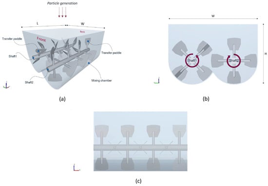
Figure 1.
(a) Isometric view, (b) front view and (c) side view of the paddle mixer. For clarity, only shaft 2 is shown in the side view.
To avoid accumulation in the corners of the mixing chamber, the last two paddles are positioned in the opposite direction with a 15 deg angle and serve as ’transfer’ paddles (Figure 1a). To avoid collisions between the paddles of the two shafts, a phase angle of 45 deg is applied (Figure 1b). The dimensions of the mixing chamber are listed in Table 1. Detailed dimensions of the shaft and paddles are left out due to confidentiality reasons. The DEM input parameters of this study are listed in Table 2.

Table 1.
Dimensions of the paddle mixer as shown in Figure 1.
Table 2.
Discrete element method (DEM) input parameters. The Poisson’s ratio, , and the shear modulus, , are adopted from [29].
The input parameters are mainly adopted from the calibrated and validated model of Jadidi et al. [4]. Moreover, a time step, , of 4.74378 × 10⁻⁵ s and a shear modulus, , of 1 × 10⁶ Pa were used for all simulations in the experimental simulation plan based upon a conducted stability analysis. The geometric properties are based upon the material stainless steel 304 [29].
The simulation was started with a particle generation process called the filling process and the actual mixing process of the binary granular material. A static factory was used to randomly generate spherical particles with a downward velocity of 2 m/s (-Z direction in Figure 1). After a gravitational settling process for approximately 3 s, the particle bed reaches a steady state while the impellers remain stationary.
The steady state is defined as the moment when the particle bed reaches a kinetic energy/potential energy ratio equal to or lower than 1 × 10⁻⁶ [30].
The number of particles follows from the input settings (particle diameter, composition and fill level). The mesh size is equal to 3Rmin. Thereafter, the shafts start to rotate according to a predetermined impeller rotational speed for 60 s.
To be able to assess the overall mixing performance of the system in a quantitative manner, a so-called mixing index is required. Typical characteristics of such an index include mixing process independence, ease of determination and accurate representation of the resulting mixing quality [31].
Bhalode et al. [32] carried out a comprehensive review of different mixing indices available in the literature and classified them into three main categories, namely variance-based, distance-based and contact-based indices. Due to their simplicity, variance-based indices are most widely used to evaluate the mixer performance. However, they are highly dependent on the grid size of the system. A small grid size could overlook a sufficient mixture on a macro-scale level, while a coarse grid could miss micro-mixing effects. Therefore, in case a variance-based index is utilized, it is necessary to conduct a grid size analysis. The distance-based indices use the distance between particles belonging to different mixture components to measure the mixing quality of the (final) product. Although these indices are grid independent, they are computationally expensive and hard to implement compared to variance-based indices. Contact-based indices utilise the contacts of a singular particle with neighbouring particles to measure mixing. Although easy to calculate in DEM, these indices are impossible to measure in experiments and hence are not suitable for validation of the DEM model with experimental results. Additionally, in the granular dilute regime, where particles are far from each other in fluidized beds/zones, contact-based indices yield erroneous results.
As a result, the distance- and contact-based mixing indices are not suitable for this study since they are not only computationally expensive but also direction dependent and misleading in dilute regimes. Thus, the variance-based mixing indices are employed in the present study. According to Emmerink [33], all indices belonging to the variance-based set, excluding the mixing segregation index (MSI), are applicable.
Here, the relative standard deviation (RSD) and Lacey’s index (LI) are used to assess the mixing performance of the system. These indices are frequently used [3,10,20,23,34,35] and calculated by Equations (9) and (11). Theoretically, an RSD of one indicates a completely segregated mixture and an RSD of zero indicates a perfectly mixed mixture.
where is the standard deviation and is the average concentration over all evaluated bins. The standard deviation is calculated by Equation (10).
where and represent the total number of evaluated bins and the average particle concentration of bin , respectivelt. The concentrations in Equations (9) and (10) are defined as the number of particles of component 1 divided by the number of particles of component 2.
LI provides an indication of the mixture’s state as well but differs in definition. An LI of zero means a completely segregated mixture and an LI of one means perfectly mixed.
where and represent variances of the mixture where the subscripts and indicate a completely segregated state or perfectly mixed state. The variables and are calculated by Equations (12)–(14).
where is the average number of particles in a bin.
2.3. Plackett–Burman (P–B)
A two-level Plackett–Burman (P–B) was selected to conduct the design of experiments (DoE). The P–B design statistically examines the significance of factors and screens the most significant ones in the least number of runs, which is desirable due to the high computational time of DEM simulations. An N-run P–B design is suitable to study up to (N − 1) factors at two levels [36]. In this study, a 12-run P–B design was used to investigate nine factors as listed in Table 3. Besides the nine factors, two virtual factors (i.e., X1 and X2) were included to complete the P–B design. Altair’s HyperStudy v2022.1 was used to conduct the P–B design.
Table 3.
Factors with corresponding levels for the Plackett–Burman (P–B) Design of Experiments (DoE).
Figure 2 visually presents most of the factor levels presented in Table 3. The composition is the total particle volume ratio between component 2 divided by component 1. In the Plackett–Burman DoE, for 6 out of 12 runs, the composition is defined as the volume ratio of small particles (component 2) to large particles (component 1). Furthermore, the initial filling patterns are defined as Front-Bottom (FB) and Top-Bottom (TB) as shown in Figure 2b. A 100% fill level is equal to the occupied bulk volume up to 107% of the shaft height. The maximum fill level of 140% is based on practice. With respect to the paddle size, the upper and lower values of the effective paddle surface were defined according to the reference paddle size shown in Figure 2d. It is important to note that for the geometric parameters, the “transfer paddle” pairs on both shafts remain unchanged.
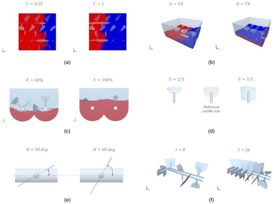
Figure 2.
Illustrations of factor levels: (a) composition, (b) initial filling pattern (FB = Front-Back, TB = Top-Bottom), (c) fill level, (d) paddle size, (e) paddle angle and (f) paddle number.
Four key performance indicators (KPIs) were formulated to assess the mixing performance in terms of mixing quality, mixing time, average mixing power per kilogram and total energy consumption per kilogram. The LI outputs could not differentiate between the state of the mixing in twelve runs (i.e., LI values had a range of 0.84–0.99) and therefore, LI was not used for the analysis. Thus, four KPIs were formulated based on the RSD as follows:
- KPI 1 (-) Mixing quality—Average steady-state RSD;
- KPI 2 (s) Mixing time—Time required to reach a steady-state RSD;
- KPI 3 (W/kg) Normalized average power—Average energy per second per kilogram over a full mixing period;
- KPI 4 (J/kg) Total energy consumption—Required energy to reach a steady state RSD.
To calculate KPI 1, the RSD should have reached a constant value known as a steady state (cf. Figure 3). Qualitatively, the steady-state period is identified by visually assessing the RSD time plots. To account for fluctuations, the average RSD is calculated over the last 10 s of mixing. In addition to KPI 1, KPI 2 is very sensitive to fluctuations. To address this issue, an upper and lower margin of 15% on the average steady-state RSD is defined to take into account these fluctuations (Figure 3). The KPI 2 calculation method for run 4, run 7 and run 10 does not hold because of the weak decline in RSD over time. To ensure consistency between all runs, the KPI 2 values were manually determined for these three runs. KPI 3 is calculated by extracting the torque values experienced by both paddle mixer shafts from EDEM and multiplying them with the constant rotation angle for every time step. The consumed energy is then divided by the total mixing time and the mass of the granular material in the system. KPI 4 is calculated by the multiplication of KPI 2 and KPI 3.
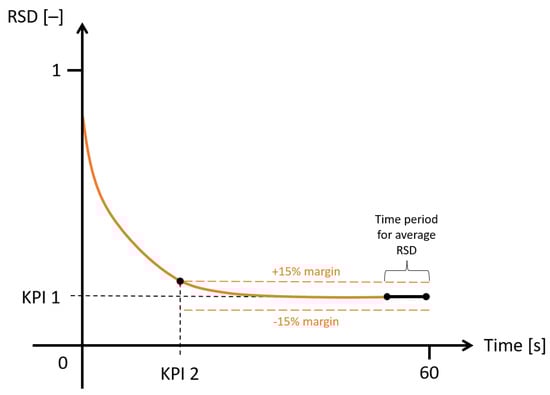
Figure 3.
Schematic of the definition KPI 1 and KPI 2 from an RSD-Time plot.
2.4. Grid System
The RSD is highly dependent on the number of bins and bin size of the grid system. To select a suitable grid system for all twelve simulations, a grid system analysis was conducted on the worst-case situation, defined as the simulation run with the largest particle size and lowest particle number (run 5). The eight different grid systems are evaluated and shown in Table 4.
Table 4.
Influence of grid system on KPI 1 for run 5.
A threshold value is determined to eliminate bins filled with particles lower than the average number of particles over all bins [12,32,37]. The 7 × 7 × 4 to 9 × 9 × 6 grid systems yield approximately a 0.17 ± 0.01 (average) steady-state RSD. A lower or higher number of bins results in a higher deviation of 0.03. The 8 × 8 × 5 grid system maintains a sufficient balance between macro- and micro-mixing mechanisms and is therefore chosen as a suitable grid system.
2.5. Granular Temperature
The granular temperature indicates the mobility of bulk material in a certain control volume. The velocities of particles in any direction in a given time period are used to calculate this macroscopic characteristic [10] as follows:
where u′ represents the fluctuation velocity of each particle at a given time and control volume and the triangular brackets ⟨⟩ function as temporal averaging within the control volume [4,10,38]. In general, the granular temperature is heavily related to the diffusive mixing mechanism of a mixing application [10]. A higher granular temperature means higher velocity fluctuations. In other words, particles behave in a chaotic and inconsistent way. To improve the understanding of the mixing mechanism in the paddle mixer and its relationship with the constructed KPIs, granular temperature data will be extracted from the DEM software. In this study, the granular temperature is used to provide further insights and support conclusions based on the KPIs.
As the granular temperature is highly dependent on the control volume and the time step, a number of steps are conducted. The used DEM software provides granular temperature extraction from evaluation points [39]. A distance-weighted sum of the particle data is performed using a normal weighting function, calculated by Equation (16), to obtain continuum temperature data between the evaluation points [39].
where ϕ is the normal distribution function and is the distance of a given particle from the evaluation point. The cut off distance identifies the width of the normal distribution function with a confidence interval equal to 99% [39]. Alternatively, from a more practical point of view, the cut off distance is equal to the radius of the spherical control volume of one single evaluation point.
It is recommended to use at least a cut off distance equal to 9 times the average particle diameter in the system [39]. To find a suitable cut off distance, the worst-case scenario is considered. Therefore, run 1 is chosen for finding a suitable cut off distance as this run consists of both particle diameters of 5 and 15 mm. For every run, a cut off distance of 25 mm is determined, where the evaluation points are a 2*cut off distance apart from each other. This comes down to a total number of 18 evaluation points over the length of the paddle mixer. To reduce the calculation time of each run, data are saved every 2 s. Consequently, a time step of 2 s was selected to obtain an average granular temperature over the full mixing period.
Three locations are selected for granular temperature assessment: location 1 (Loc_1), between the shafts, and two locations (Loc_2 and Loc_3) at the bottom, illustrated in Figure 4a. All three locations are characterized by different particle behaviour according to visual observations of the particle bed. Loc_1 represents the fluidized zone, Loc_2 the compressed state before the material is thrown into the centre of the mixing chamber and Loc_3 represents the location where the particles fall down onto the quasi-static particle bed. The granular temperature results should align with the aforementioned observations. The 18 evaluation points are evenly distributed on the red lines illustrated in Figure 4b. The average granular material for all evaluation points is gathered for every location and every run. The results can be found in the Results and Discussion section.
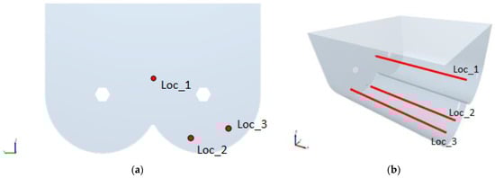
Figure 4.
Location identification for granular temperature extraction. (a) Front view of paddle mixer with location IDs and (b) isometric view of paddle mixer where the evaluation points are equally distributed on the red lines.
3. Results and Discussion
The Plackett–Burman (P–B) Design of Experiments (DoE) is shown in Table 5. The outputs of the P–B DoE are presented by KPI 1, KPI 2, KPI 3 and KPI 4. The RSD–Time plots for all twelve simulations are presented in Figure 5. As can be seen, all simulations were carried out for 60 s except run 4 and 11, where they were continued for 150 and 120 s to ensure that a steady state was reached. The results of the P–B DoE were analysed using a Pareto plot in conjunction with an analysis of variance (ANOVA) analysis for each KPI individually. The former presents the factors’ order of significance, while the latter shows the statistical significance of each factor separately. Usually, a p-value of 0.05, equivalent to a confidence interval (CI) of 95%, is used as a cut off to detect significant factors. However, a p-value of 0.1 is used in this study due to the fact that P–B DoE is not able to capture interactions between factors. In other words, the null hypothesis that the factor of interest does not have an effect on the response parameter can be rejected with 90% CI (or p < 0.1) [40].
Table 5.
Plackett–Burman (P–B) design with the resulting key performance indicators (KPIs); KPI 1 = average steady-state relative standard deviation (RSD); KPI 2 = time required to reach a steady-state RSD; KPI 3 = average energy per second per kilogram over full mixing period; KPI 4 = required energy to reach a steady state RSD.
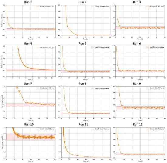
Figure 5.
RSD–Time plots of all twelve runs as in Table 5.
3.1. KPI 1: Mixing Quality
Figure 6 presents the Pareto plot of the P–B analysis of KPI 1, which shows the order of factors’ significance on the steady-state RSD value. The blue line denotes the accumulation of the total effect and the dashed lines in the bars denote a positive (+) or negative (−) correlation with the respective KPI. As for the small bars in the Pareto plot, the dashed lines are not visible, for each KPI an extra figure is added, indicating the main effect of factors on the respective KPI. As can be seen, the paddle angle has the largest effect on KPI 1 followed by the impeller rotational speed, paddle number and fill level. The ANOVA results presented in Table 6 show the factor’s significance. The R squared value indicates an accurate fit with the obtained data. Considering the cut off value of 0.1 for the p-value, only the paddle angle has a significant effect and is positively correlated with KPI 1.
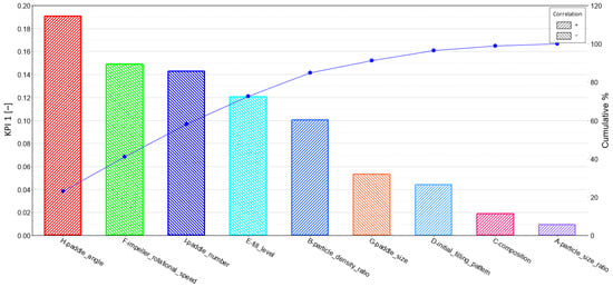
Figure 6.
The Pareto plot of KPI 1 mixing quality.
Table 6.
Analysis of variance (ANOVA) results of KPI 1 mixing quality.
Furthermore, Figure 7 shows the negatively correlated fill level, impeller rotational speed and paddle number meaning that an increase in these factors leads to a decrease in KPI 1 (thus an improvement in mixing quality).
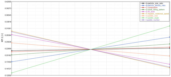
Figure 7.
Main effect of factors on KPI 1 mixing quality.
On the contrary, the paddle angle shows a positive correlation, which means that an increase in paddle angle leads to an increase in KPI 1 (thus a deterioration in the mixing quality). The material properties have a minor effect on the mixing quality, while the operational conditions and geometric parameters have a relatively significant role in this measure of mixing performance.
A comparison with the literature shows at first sight inconclusive results. Studies on other types of mixers showed the importance of the impeller configuration in terms of paddle angle in a single-shaft paddle mixer [14], and showed that the initial filling pattern does not significantly influence the mix quality for a single-shaft paddle mixer [3] and for a ploughshare mixer [12].
For the double-paddle mixer, Jadidi et al. [4] found that the initial filling pattern does have an effect on the mixing performance. However, this is in contrast with the results of this research, where we show that the initial filling pattern has no significant effect on the mixing index (KPI 1). This can be explained by the differences in paddle angles in both studies. In this study, the angled paddles cause particle dispersion in both the radial and axial directions, while Jadidi et al. [4] used paddles that are in line with the shaft, resulting in a very low axial dispersion.
The results show that the impeller rotational speed is the second most influential on KPI 1. From the literature [16], its significance was also found for another agitated mixer, namely the ribbon mixer in a double u-shaped vessel. According to Gao et al. [16], the mixing quality improves with an increase in the impeller rotational speed. Jadidi et al. [4] found contradictory results, where the impeller rotational speeds of 40 and 70 rpm with a TB initial filling pattern eventually approach the same steady-state RSD.
3.2. KPI 2: Mixing Time
With respect to the time it takes for a steady-state RSD to be reached (KPI 2), the Pareto plot and ANOVA results are shown in Figure 8 and Table 7. The ANOVA results show none of the factors are significant over the others. Nevertheless, the Pareto plot presents the order of significance, with the impeller rotational speed affecting KPI 2 the most. In Figure 9, the main (linear) effect of the factors is shown on KPI 2. Considering only the first few factors in the order of significance, the particle size ratio and impeller rotational speed are negatively correlated with KPI2, while the fill level is positively correlated. The increase in impeller rotational speed results in reaching the steady-state RSD faster (Figure 9), which is in line with the literature on double-shaft paddle mixers [4,12,20]. However, Qi et al. [18] investigated a double shaft, lab-scale screw mixer and found that the screw’s rotational speed did not affect the mixing time nor the mixing quality with a constant fill level and screw pitch.
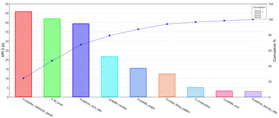
Figure 8.
Pareto plot for KPI 2 mixing time.
Table 7.
Analysis of variance (ANOVA) results of KPI 2 mixing time.
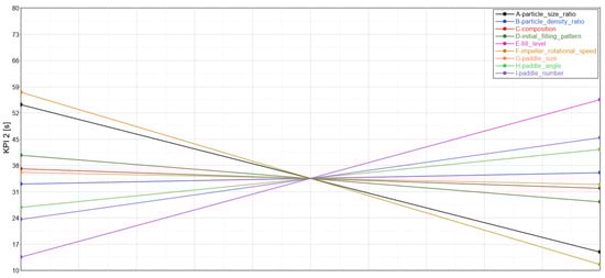
Figure 9.
The main effect of factors on KPI 2 mixing time.
Furthermore, according to Jadidi et al. [4], the fill level had no significant effect on the mixing performance. On the contrary, a study by Alian et al. [12] on a single-shaft ploughshare mixer showed that the fill level had an effect on the mixing time. They stated that it was due to the difference in free space for the particles to move through in the agitated vessel. This research shows that the fill level has a positive correlation with KPI 2; thus, increasing the fill level leads to an increase in KPI 2. In other words, the time it takes to reach a steady-state RSD increases with an increase in the fill level.
3.3. KPI 3: Average Mixing Power Per Kilogram
This KPI (as well as KPI 4) has been formulated to examine the performance of the mixer with respect to sustainability. To the best of the authors’ knowledge, there is no research work exploring the energy efficiency of paddle mixers. Having a deep understanding of the main factors influencing the energy consumption of paddle mixers paves the way for optimising this device from an environmental point of view. KPI 3 was defined as the total energy consumed by the mixer normalised by the mixing time and mass of the materials. The results of the P–B design regarding KPI 3 are presented in Figure 10 and Table 8.
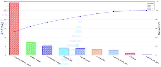
Figure 10.
Pareto plot for KPI 3 average mixing power.
Table 8.
Analysis of variance (ANOVA) results of KPI 3 average mixing power.
Figure 10 clearly shows that the impeller rotational speed, as expected, has the biggest contribution to the energy consumption. Besides this factor, the ANOVA presented in Table 8 confirms the significance of the paddle number, initial filling pattern, paddle size, paddle angle and composition (considering a p-value < 0.1). This implies that while both operational and geometric parameters are essential for the energy efficiency of the mixer, the material properties have a small effect. In other words, one should put emphasis on operational and geometric parameters for the purpose of optimising the mixer with respect to energy consumption. For instance, based on Figure 11, it can be initially recommended to utilise a lower number of paddles with a bigger size and a higher angle to minimise the energy consumed by the mixer.
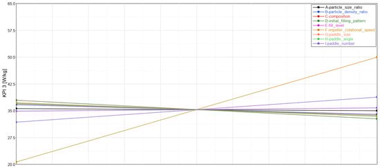
Figure 11.
The main effect of factors on KPI 3 average mixing power.
3.4. KPI 4: Total Mixing Energy Required to Reach a Steady-State RSD
KPI 4 represents the total mixing energy and is defined as a multiplication of KPI 2 (mixing time) and KPI 3 (average mixing power). It was formulated this way to examine how much energy is consumed to reach a steady-state RSD, which is becoming an increasingly important factor in the mixing process. The results of the P–B design for KPI 4 are shown in Figure 12 and Table 9.
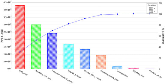
Figure 12.
The Pareto plot for KPI 4 total energy consumption.
Table 9.
Analysis of variance (ANOVA) results of KPI 4 total energy consumption.
As can be seen, the fill level shows the most contribution to the amount of energy required to reach a steady state. In addition, although KPI 3 and KPI 4 are similar, as both deal with energy consumption, the order of significance of factors for KPI 4 is very different from that for KPI 3. This is because in KPI4, besides the mixing energy, the mixing time has also been considered. An interesting observation was that by increasing the impeller rotational speed from 40 to 80 rpm, the amount of energy required to reach the steady-state RSD decreases (Figure 13). This can be explained by the fact that the impeller rotational speed has an opposing effect on KPI 2 (mixing time) and KPI 3 (mixing energy), and it can be concluded that its effect on KPI 2 is more pronounced. Additionally, it can be seen that in both cases, the mixing energy and mixing time are of interest for optimization, the geometric parameters (i.e., paddle angle and paddle size) have a negligible effect and operational conditions such as fill level and impeller rotational speeds should be focused on.
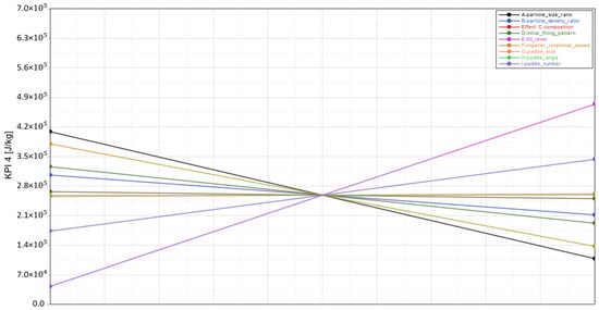
Figure 13.
The main effect of factors on KPI 4 total energy consumption.
3.5. Summary of Results of the P–B Design
The factors investigated from three different groups (material properties, operational conditions and geometric parameters) show distinctive behaviour depending on the response variable. In Table 10, a summary of all results is presented. It should be noted that the statistical significance of a factor (p < 0.1) is indicated by three pluses/minuses. A lower number of respective symbols (two or one) denotes the factor’s order of significance.
Table 10.
Summary of factor response. Pluses (+) and minuses (−) indicate positive and negative correlations, respectively. The number of pluses and minuses indicates the factor’s significance, e.g., (+++), (++) and (+) indicate p < 0.1, 0.1 ≤ p < 0.2 and p ≥ 0.2, respectively.
3.6. Granular Temperature
The granular temperature results for the three specified locations in the paddle mixer are shown in Table 11.
Table 11.
Results of the average granular temperature over the length of the paddle mixer. The three different locations are the fluidized zone (Loc_1) and at the bottom left (Loc_2) and bottom right (Loc_3). See Figure 4 for the definition of the locations Loc_1, Loc_2 and Loc_3.
First, for almost all runs it can be observed that the granular temperature is higher in the centre (Loc_1) of the mixing chamber (also called the fluidized zone) compared to the bottom locations (Loc_2 and Loc_3). This observation confirms the expected trend where the particulate behaviour is mostly dynamic at the fluidized zone being formed between two paddles. Second, Loc_2 exhibited the lowest granular temperature in nearly all cases. This is due to the quasi-static state of the granular material before being thrown into the fluidized zone of the mixing chamber. Third, it can be observed for the fluidized zone of the mixing chamber (Loc_1) that the granular temperature can be related to the mixing time (KPI 2) of the paddle mixer. For instance, run 4 and run 11, which are characterized by a very long mixing time, have a very low granular temperature compared to other runs. Thus, a low diffusive behaviour of particles in the fluidized zone affects the mixing time in a negative way.
4. Conclusions
In this study, the discrete element method (DEM) and Plackett–Burman (P–B) design were used to investigate the mixing performance of a double paddle mixer. To this end, several material properties (i.e., particle size ratio, density ratio and composition), operational conditions (i.e., filling pattern, fill level and impeller rotational speed) and geometric parameters (i.e., paddle size, angle and number) were examined. In order to quantitatively analyse their effects on mixing performance, a number of key performance indicators (KPIs) were defined, namely the average steady-state RSD (KPI 1), the mixing time (KPI 2) and the average mixing power (KPI 3). In addition, KPI 4 was formulated as a multiplication of KPI 2 and KPI 3 to examine the mixing time and energy consumption at the same time.
The results were analysed using Pareto plots in conjunction with ANOVA analyses. Furthermore, the time-averaged granular temperature was assessed in three spatial locations for all different runs to verify the observations with respect to the RSD. The main findings can be summarised as follows:
- Taking all KPIs into account, it can be generally concluded that material properties in the range investigated here do not significantly influence the mixer performance. In other words, when a mixer is well-designed, it will perform equally well in the range of material properties explored in this work. Nevertheless, it was found that a 50/50 volume ratio between components 1 and 2 needs less average mixing power (i.e., KPI 3) compared to an 20/80 composition.
- Increasing the fill level enhances the mixing quality, but at the same time sacrifices a fast mixing time and a low total energy consumption. In addition, an increase in the impeller rotational speed leads to a mixing quality improvement, higher mixing time and lower total energy consumption. In short, a lower fill level in combination with a high rotational speed could lead to improved mix qualities, achieved in a faster and more sustainable way.
- With respect to geometric parameters, the paddle angle is the most influential, where a decrease in the paddle angle significantly improves the mixing quality without compromising the mixing time or total energy consumption. Additionally, the paddle number seems to affect the mixing quality, but more research is required to confirm the aforementioned relation.
- While increasing the paddle size significantly decreases the energy consumption, it does not greatly affect the mixing quality and mixing time, meaning that this factor holds great potential to be optimised for both efficient and sustainable double paddle mixers.
- A granular temperature analysis showed an interesting relation between mixing time (KPI 2) and diffusivity in the fluidized zone of the paddle mixer. It was found that the mixing time is affected negatively when the fluidized zone is characterized by a low diffusive mixing mechanism.
- Overall, one should focus on operational conditions and geometric parameters when all the KPIs, including the mixing quality, mixing time and energy consumption, are of interest for the purpose of process optimisation.
It should also be noted that due to the high number of factors studied in this work, the P–B design was used, which has the drawback of neglecting the interactions between factors. Additionally, when using a P–B design with two factors, one of the assumptions is that the behaviour of the system between the two levels is linear, which is often not the case, as shown in [33]. Therefore, it is recommended to explore the factor space with at least three levels to capture possible non-linear behaviour. Additionally, it is worthwhile to focus on the operational conditions and geometric parameters in future work to further optimise the mixing process.
Author Contributions
Conceptualization, J.E., A.H., C.C. and D.L.S.; formal analysis, J.E.; investigation, J.E. and D.L.S.; methodology, J.E. and A.H.; resources, C.C. and D.L.S.; software, J.E.; supervision, A.H., J.J., C.C. and D.L.S.; visualization, J.E.; writing—original draft, J.E. and A.H.; writing—review and editing, J.J., C.C. and D.L.S. All authors have read and agreed to the published version of the manuscript.
Funding
This research received no funding.
Data Availability Statement
The data presented in this study are available on request from the corresponding author. The raw data are not publicly available due to confidentiality reasons.
Conflicts of Interest
The authors declare no conflict of interest.
References
- Rhodes, M.J. Introduction to Particle Technology; John Wiley & Sons: Hoboken, HJ, USA, 2008. [Google Scholar]
- Paul, E.L.; Atiemo-Obeng, V.A.; Kresta, S.M. Handbook of Industrial Mixing: Science and Practice; John Wiley & Sons: Hoboken, HJ, USA, 2003. [Google Scholar]
- Ebrahimi, M.; Yaraghi, A.; Jadidi, B.; Ein-Mozaffari, F.; Lohi, A. Assessment of bi-disperse solid particles mixing in a horizontal paddle mixer through experiments and DEM. Powder Technol. 2021, 381, 129–140. [Google Scholar] [CrossRef]
- Jadidi, B.; Ebrahimi, M.; Ein-Mozaffari, F.; Lohi, A. Mixing performance analysis of non-cohesive particles in a double paddle blender using DEM and experiments. Powder Technol. 2022, 397, 117122. [Google Scholar] [CrossRef]
- Bagster, D.; Bridgwater, J. The measurement of the force needed to move blades through a bed of cohesionless granules. Powder Technol. 1967, 1, 189–198. [Google Scholar] [CrossRef]
- Bagster, D.; Bridgwater, J. The flow of granular material over a moving blade. Powder Technol. 1969, 3, 323–338. [Google Scholar] [CrossRef]
- Stewart, R.; Bridgwater, J.; Parker, D. Granular flow over a flat-bladed stirrer. Chem. Eng. Sci. 2001, 56, 4257–4271. [Google Scholar] [CrossRef]
- Conway, S.L.; Lekhal, A.; Khinast, J.G.; Glasser, B.J. Granular flow and segregation in a four-bladed mixer. Chem. Eng. Sci. 2005, 60, 7091–7107. [Google Scholar] [CrossRef]
- Lekhal, A.; Conway, S.L.; Glasser, B.J.; Khinast, J.G. Characterization of granular flow of wet solids in a bladed mixer. AIChE J. 2006, 52, 2757–2766. [Google Scholar] [CrossRef]
- Boonkanokwong, V.; Remy, B.; Khinast, J.G.; Glasser, B.J. The effect of the number of impeller blades on granular flow in a bladed mixer. Powder Technol. 2016, 302, 333–349. [Google Scholar] [CrossRef]
- Cundall, P.A.; Strack, O.D.L. A discrete numerical model for granular assemblies. Géotechnique 1979, 29, 47–65. [Google Scholar] [CrossRef]
- Alian, M.; Ein-Mozaffari, F.; Upreti, S.R. Analysis of the mixing of solid particles in a plowshare mixer via discrete element method (DEM). Powder Technol. 2015, 274, 77–87. [Google Scholar] [CrossRef]
- Chandratilleke, G.; Dong, K.; Shen, Y. DEM study of the effect of blade-support spokes on mixing performance in a ribbon mixer. Powder Technol. 2018, 326, 123–136. [Google Scholar] [CrossRef]
- Ebrahimi, M.; Yaraghi, A.; Ein-Mozaffari, F.; Lohi, A. The effect of impeller configurations on particle mixing in an agitated paddle mixer. Powder Technol. 2018, 332, 158–170. [Google Scholar] [CrossRef]
- Laurent, B.; Cleary, P. Comparative study by PEPT and DEM for flow and mixing in a ploughshare mixer. Powder Technol. 2012, 228, 171–186. [Google Scholar] [CrossRef]
- Gao, W.; Liu, L.; Liao, Z.; Chen, S.; Zang, M.; Tan, Y. Discrete element analysis of the particle mixing performance in a ribbon mixer with a double U-shaped vessel. Granul. Matter 2019, 21, 12. [Google Scholar] [CrossRef]
- Hassanpour, A.; Tan, H.; Bayly, A.; Gopalkrishnan, P.; Ng, B.; Ghadiri, M. Analysis of particle motion in a paddle mixer using Discrete Element Method (DEM). Powder Technol. 2011, 206, 189–194. [Google Scholar] [CrossRef]
- Qi, F.; Heindel, T.J.; Wright, M.M. Numerical study of particle mixing in a lab-scale screw mixer using the discrete element method. Powder Technol. 2017, 308, 334–345. [Google Scholar] [CrossRef]
- Jadidi, B.; Ebrahimi, M.; Ein-Mozaffari, F.; Lohi, A. Investigation of impacts of particle shape on mixing in a twin paddle blender using GPU-based DEM and experiments. Powder Technol. 2023, 417, 118259. [Google Scholar] [CrossRef]
- Jadidi, B.; Ebrahimi, M.; Ein-Mozaffari, F.; Lohi, A. Mixing and segregation assessment of bi-disperse solid particles in a double paddle mixer. Particuology 2023, 74, 184–199. [Google Scholar] [CrossRef]
- Jadidi, B.; Ebrahimi, M.; Ein-Mozaffari, F.; Lohi, A. A comprehensive review of the application of DEM in the investigation of batch solid mixers. Rev. Chem. Eng. 2022. [Google Scholar] [CrossRef]
- Pantaleev, S.; Yordanova, S.; Janda, A.; Marigo, M.; Ooi, J.Y. An experimentally validated DEM study of powder mixing in a paddle blade mixer. Powder Technol. 2017, 311, 287–302. [Google Scholar] [CrossRef]
- Tsunazawa, Y.; Soma, N.; Sakai, M. DEM study on identification of mixing mechanisms in a pot blender. Adv. Powder Technol. 2022, 33, 103337. [Google Scholar] [CrossRef]
- Yuan, Q.; Xu, L.; Ma, S.; Niu, C.; Yan, C.; Zhao, S. The effect of paddle configurations on particle mixing in a soil-fertilizer continuous mixing device. Powder Technol. 2021, 391, 292–300. [Google Scholar] [CrossRef]
- Alchikh-Sulaiman, B.; Ein-Mozaffari, F.; Lohi, A. Evaluation of poly-disperse solid particles mixing in a slant cone mixer using discrete element method. Chem. Eng. Res. Des. 2015, 96, 196–213. [Google Scholar] [CrossRef]
- Shenoy, P.; Xanthakis, E.; Innings, F.; Jonsson, C.; Fitzpatrick, J.; Ahrné, L. Dry mixing of food powders: Effect of water content and composition on mixture quality of binary mixtures. J. Food Eng. 2015, 149, 229–236. [Google Scholar] [CrossRef]
- Grima, A. Quantifying and Modelling Mechanisms of Flow in Cohesionless and Cohesive Granular Materials. Ph.D. Thesis, University of Wollongong, Wollongong, Australia, January 2011. Available online: https://ro.uow.edu.au/theses/3425 (accessed on 9 March 2022).
- Forberg, H.G. Twin Horizontal Axled Inwardly Rotating Paddle Mixer for Dry Ingredients. Canada Patent CA1143372 (A), 22 March 1983. [Google Scholar]
- AZO Materials, ‘Stainless Steel–Grade 304 (UNS S30400)’, AZoM.com. 23 October 2001. Available online: https://www.azom.com/article.aspx?ArticleID=965 (accessed on 7 December 2022).
- Lommen, S.; Schott, D.; Lodewijks, G. DEM speedup: Stiffness effects on behavior of bulk material. Particuology 2014, 12, 107–112. [Google Scholar] [CrossRef]
- Poux, M.; Fayolle, P.; Bertrand, J.; Bridoux, D.; Bousquet, J. Powder mixing: Some practical rules applied to agitated systems. Powder Technol. 1991, 68, 213–234. [Google Scholar] [CrossRef]
- Bhalode, P.; Ierapetritou, M. A review of existing mixing indices in solid-based continuous blending operations. Powder Technol. 2020, 373, 195–209. [Google Scholar] [CrossRef]
- Emmerink, J. Parametric Analysis of a Double Shaft Batch-Type Paddle Mixer: A DEM Study. 2022. Available online: https://repository.tudelft.nl/islandora/object/uuid%3A940bb90b-183a-4e00-bd1c-aee2f455b3f9 (accessed on 1 February 2023).
- Basinskas, G.; Sakai, M. Numerical study of the mixing efficiency of a ribbon mixer using the discrete element method. Powder Technol. 2016, 287, 380–394. [Google Scholar] [CrossRef]
- Tsugeno, Y.; Sakai, M.; Yamazaki, S.; Nishinomiya, T. DEM simulation for optimal design of powder mixing in a ribbon mixer. Adv. Powder Technol. 2021, 32, 1735–1749. [Google Scholar] [CrossRef]
- Antony, J. Design of Experiments for Engineers and Scientists; Elsevier: London, UK, 2014. [Google Scholar]
- Boukouvala, F.; Gao, Y.; Muzzio, F.; Ierapetritou, M.G. Reduced-order discrete element method modeling. Chem. Eng. Sci. 2013, 95, 12–26. [Google Scholar] [CrossRef]
- Remy, B.; Khinast, J.G.; Glasser, B.J. Discrete element simulation of free flowing grains in a four-bladed mixer. AIChE J. 2009, 55, 2035–2048. [Google Scholar] [CrossRef]
- Altair EDEM 2022. Available online: https://2022.help.altair.com/2022.1/EDEM/index.htm#t=Getting_Started.htm (accessed on 6 February 2023).
- Fang, M.; Yu, Z.; Zhang, W.; Cao, J.; Liu, W. Friction coefficient calibration of corn stalk particle mixtures using Plackett-Burman design and response surface methodology. Powder Technol. 2021, 396, 731–742. [Google Scholar] [CrossRef]
Disclaimer/Publisher’s Note: The statements, opinions and data contained in all publications are solely those of the individual author(s) and contributor(s) and not of MDPI and/or the editor(s). MDPI and/or the editor(s) disclaim responsibility for any injury to people or property resulting from any ideas, methods, instructions or products referred to in the content. |
© 2023 by the authors. Licensee MDPI, Basel, Switzerland. This article is an open access article distributed under the terms and conditions of the Creative Commons Attribution (CC BY) license (https://creativecommons.org/licenses/by/4.0/).