Pixel-Level Concrete Crack Segmentation Using Pyramidal Residual Network with Omni-Dimensional Dynamic Convolution

Abstract

Automated crack detection technologies based on deep learning have been extensively used as one of the indicators of performance degradation of concrete structures. However, there are numerous drawbacks of existing methods in crack segmentation due to the fine and microscopic properties of cracks. Aiming to address this issue, a crack segmentation method is proposed. First, a pyramidal residual network based on encoder–decoder using Omni-Dimensional Dynamic Convolution is suggested to explore the network suitable for the task of crack segmentation. Additionally, the proposed method uses the mean intersection over union as the network evaluation index to lessen the impact of background features on the network performance in the evaluation and adopts a multi-loss calculation of positive and negative sample imbalance to weigh the negative impact of sample imbalance. As a final step in performance evaluation, a dataset for concrete cracks is developed. By using our dataset, the proposed method is validated to have an accuracy of 99.05% and an mIoU of 87.00%. The experimental results demonstrate that the concrete crack segmentation method is superior to the well-known networks, such as SegNet, DeeplabV3+, and Swin-unet.

1. Introduction

Cracks in concrete are considered as a significant flaw when inspecting civil engineering projects. From an engineering perspective, fractures affect not only the stability and longevity of engineering constructions, but also the durability of concrete [1], which may be caused by small or massive cracks that slowly spread and cause the final collapse or destruction of the structure. Currently, the primary approaches to detect crack-like flaws refer to simple instrumental measurements and visual inspection. The latter, however, is considered as an arduous operation. Moreover, there may be significant misdetection and omission in some regions with problems [2]. Manual crack detection is not ideal for mass detection since it frequently encounters problems such as heavy workload, complex structure, and inconsistent evaluation standards. Compared with manual inspection, machine vision inspection shows the features of efficiency as well as safety and reliability due to its lack of contact with the object. Traditional machine vision methods have been extensively used to solve industrial problems, including object inspection [3], material contour measurement [4], distance measurement [5], etc. For example, multi-vision measurement methods can be used to accurately measure the surface deformation and full-field strain values of steel pipe concrete columns [6]. The use of exponential functional density clustering models can perform better than the clustering and deep learning (DL) methods for indoor object extraction tasks [7]. Despite the considerable achievements, conventional vision technologies still require expert analysis and fine-tuning for their application, making them inappropriate for complex problems. Due to the continuous innovation and development of digital images, the combination of digital image processing methods and DL in the engineering structural defect detection industry is a new research direction in crack inspection technology in recent years. Then, the DL algorithms for autonomous detection are used to identify the target defects on the surface of the engineering structure rather than identifying them based on the artificial experience of using an unmanned aerial vehicle [8] or a wall-climbing robot [9] carrying relevant equipment to capture a significant amount of image data on the surface of engineering structures. In recent years, DL algorithms have made significant strides in the field of computer vision [10]. According to recent research, convolutional neural networks (CNN) can be utilized for tasks including classification [11], localization [12], and segmentation [13] in crack detection tasks. For example, researchers can augment digital image data with Generative adversarial networks (GAN) and combine them with improved visual geometry group (VGG) networks to achieve crack classification [14]. In terms of crack width measurement, a new crack width measurement method based on backbone dual-scale features can improve detection automation [15]. These studies are increasingly concentrated on employing new DL methods with successful outcomes. In certain studies on new cement repair materials, fracture segmentation algorithms based on DL have even been employed to evaluate the material performance [16].

Grey-scale segmentation, conditional random fields, and other more conventional methods constitute the majority of early segmentation algorithms, although it is very challenging to describe complicated classes using only grey-level information. With the introduction of the first semantic segmentation model based on DL, it has gained popularity in semantic segmentation tasks, that is, FCN [17], which extends end-to-end convolutional networks to semantic segmentation. To increase the efficiency of training detection with minimal datasets, an image segmentation algorithm U-Net [18] for medical image segmentation is proposed. The concept of encoder–decoder proposed by SegNet [19] is crucial to modern segmentation algorithms. Two primary optimization techniques focus on using atrous convolution and amplified convolution kernel size to successfully expand the perceptual range of feature extraction. The first is to give the network a null convolution [20]. Deeplab v1 [21], Deeplab v2 [22], DeepLab v3 [23], DeepLab v3+ [24], and DenseASPP [25] are more algorithms based on this concept. The second is to expand the convolution’s kernel size to create a wider effective receptive field [26]. Additionally, other technologies [27] make use of this concept to optimize feature extraction, and employ huge kernel pooling layers to gather these data and record the entire image. In recent years, a self-attentive semantic segmentation model [28] that employs a local-to-global approach is proposed for medical image segmentation. The success of Swin transformer in the field of image recognition shows the application potential of the transformer in vision. The main goal of these algorithms is to give the network a wider perceptual area, so as to facilitate the network to gather more global data. However, not all segmentation domains, such as crack segmentation, need global data.

The existing crack segmentation technologies can be divided into two primary groups: one is the technology of using semantic segmentation models in other domains and the other is the technology of mixing multiple networks to create a dual network for crack detection. For a crack dataset with a small amount of data, Carr et al. [29] proposed a structure with a feature pyramid core and an underlying feedforward ResNet. Yang et al. [30] proposed a pyramid and hierarchical improvement network for pavement crack detection, while Jiang et al. [31] suggested a DL-based hybrid extended convolutional block network for crack detection at the pixel level. Other effective segmentation technologies [32,33,34,35,36,37,38] likewise mostly rely on the concepts of SegNet and U-Net concepts to complete the task. Despite the excellent performance of these crack segmentation models, no studies show how the parameters of these networks affect the outcomes, for example, how much local information is collected by the network when the crack image is subjected to feature extraction, where the Skip Connection in the coding and decoding structure is located, and how many image channels are used in the feature transfer.

A pixel-level crack segmentation network (CCSN) is proposed as a solution to this issue and as a means to identify a network structure appropriate for crack segmentation. The network uses a residual network built on a feature pyramid to realize Omni-Dimensional Dynamic Convolution in the network’s fundamental block using a residual network built on a feature pyramid. The loss calculation employs a mix of the dice coefficient [39] and focal loss [40] to handle the issue of sample imbalance. The created dataset supports the claim that CCSN performs better than networks such as SegNet, DeeplabV3+, and Swin-unet. The performance of these networks is shown in Figure 1.

The main contributions of this research are summarized as follows:

1)

First, a CNN structure for crack segmentation is proposed by combining residual networks and Omni-Dimensional Dynamic Convolution. Its performance under various convolution kernels, channel numbers, connection schemes, and loss functions is thoroughly investigated to find a relatively stable and high-quality structure.

2)

Then, mIoU, mPA, and accuracy are used as the primary evaluation metrics and various loss functions are used to target binary classification and sample imbalance.

3)

Finally, a dataset for concrete cracks with distinct environments and different orientations is created and utilized for training and validation.

The remainder of this study is arranged as follows. Section 2 focuses on the work related to the method. Section 3 describes the proposed crack segmentation method in detail. Section 4 analyzes the performance of the method under different datasets. Finally, Section 5 draws the conclusion of this paper.

2. Related Work

2.1. Residual Block with ODConv

In the proposed CCSN method, the idea of Skip Connections of the residual network [41] hops is used for reference, and the Omni-Dimensional Dynamic Convolution (ODConv) [42] incorporating multi-headed attention is used.

2.1.1. Residual Network

With the increase in model layers, the problem of gradient disappearance or expansion is addressed by residual networks. Traditional neural networks frequently employ numerous convolutional layers, pooling layers, etc., especially in image processing. Since each layer takes features from the one before it, it is more likely to have problems (e.g., deterioration) as the number of layers rises. To overcome various issues of the deep neural network, the residual network adopts a Skip Connection strategy. The residual structure can be simply written in the following form:

$$x_{l+1}=x_l+F\left(x_l,W_l\right)$$

(1)

where $x_l$ is the input feature, $F\left(x_l,W_l\right)$ can be two or three convolution blocks, and $x_{l+1}$ is the output feature. Skip Connection is the direct output of layer input $x_l$ without processing plus $F\left(x_l,W_l\right)$, i.e., the layer output contains the complete input information.

2.1.2. ODConv

ODConv introduces a multi-dimensional attention mechanism with a parallel strategy to learn diverse attention of convolutional kernels along all four dimensions of kernel space.

ODConv uses an Squeeze Excitation [43] style attention module but makes it have multiple heads to compute multiple types of attention. The overall structure is shown in Figure 2. Specifically, for input, it is first shrunk by GAP to a feature vector of length and then FC is used with four heads to generate different types of attention values. Four attentional dimensions focusing on location, channel, filter, and nucleus will capture richer contextual information. ODConv leverages a novel multi-dimensional attention mechanism to compute four types of attentions ${\alpha }_{si}$, ${\alpha }_{ci}$, ${\alpha }_{fi}$, and ${\alpha }_{wi}$ for $W_i$, along with all four dimensions of the kernel space in a parallel manner. The formula is as follows:

$$y=\left({\alpha }_{w1}\odot {\alpha }_{f1}\odot {\alpha }_{c1}\odot {\alpha }_{s1}\odot W_1+\cdots +{\alpha }_{wn}\odot {\alpha }_{fn}\odot {\alpha }_{cn}\odot {\alpha }_{sn}\odot W_n\right)\ast x$$

(2)

where ∗ denotes the convolution operation and ${\alpha }_{wi}\in ℝ$ denotes the attention scalar for the convolutional kernel $W_i$; ${\alpha }_{si}\in {ℝ}^{k\times k}$, ${\alpha }_{ci}\in {ℝ}^{c_{in}}$, and ${\alpha }_{fi}\in {ℝ}^{c_{out}}$ denote three newly introduced attentions, which are computed along the spatial dimension, input channel dimension, and the output channel dimension of kernel space for the convolutional kernel $W_i$, respectively; and $\odot$ denotes the multiplication operations along different dimensions of the kernel space. Here, ${\alpha }_{si}$, ${\alpha }_{ci}$, ${\alpha }_{fi}$, and ${\alpha }_{wi}$ are computed with a multi-head attention module ${\pi }_i\left(x\right)$.

2.2. Pyramid Network

The pyramid network in our method has two levels: image pyramids [44] and feature pyramids [45]. Image pyramids are created to address the issue of multi-scale variation enhancement, where the inherent pixel information of small objects is readily lost during the process of downsampling. The multi-scale variation problem in object detection can be handled through the feature pyramids, with only a slight increase in processing effort. The feature pyramids primarily solve the weaknesses of target detection in dealing with multi-scale variation difficulties.

2.3. Loss Function

A pixel-level cross entropy (CE) loss, which analyzes each pixel separately and compares the predictions of each pixel class with our coded label vector, is the most popular loss function used for image semantic segmentation tasks. The matching loss function of each pixel is as follows:

$$\mathrm{CE}\text{\_}\mathrm{Loss}=-{\displaystyle \sum _{c=1}^M{y}_c\log (p_c)}$$

(3)

where $M$ represents the number of categories, $y_c$ is a one-hot vector with elements taking only 0 and 1 values, and $p_c$ denotes the probability that the predicted sample belongs to class $c$. When there are only two categories, the binary cross entropy (BCE) loss can be written as follows:

$$\mathrm{BCE}\text{\_}\mathrm{Loss}=-{\displaystyle \sum _{c=1}^N\left(t_c\log p_c+\left(1-t_c\right)\log \left(1-p_c\right)\right)}$$

(4)

where $p_c$ is the model input and $t_c$ is the true label. Binary cross entropy with logits (BCEL) loss combines a sigmoid layer and BCE loss into a single class. For the problem of positive and negative sample imbalance, Shrivastava et al. [46] proposed an algorithm for online hard example mining (Ohem). OhemCE loss is to calculate the cross entropy, then select hard samples according to the loss and apply higher weights to them in the subsequent training process.

Intersection over union (IoU) reflects the ratio of the intersection and merge of the true and predicted values and is commonly used as a loss function in semantic segmentation. The IoU loss expression is as follows:

$$\mathrm{IoU}\text{\_}\mathrm{Loss}=1-\frac{A\cap B}{A\cup B}$$

(5)

A loss function known as the focal loss (FL) is used to deal with the uneven classification of samples. The emphasis is to increase the weight for the loss related to the samples based on the ease of sample differentiation, which is to add smaller weights to the samples that are easy to distinguish, and to add larger weights to those that are difficult to differentiate. The expression for the loss function can then be written as

$$\mathrm{Focal}\text{\_}\mathrm{Loss}=-{\displaystyle \sum _{c=1}^M{\left(1-p_c\right)}^{\gamma }{y}_c\log p_{\mathrm{c}}}$$

(6)

FL is the addition of a weighting coefficient ${\left(1-p_c\right)}^{\gamma }$ before the standard cross entropy. Dice loss is named after the dice coefficient [47], which is a measure function used to assess the similarity of two samples. The larger value means the similarity of the two samples. The mathematical expression of the dice coefficient is as follows:

$$\mathrm{Dice}\text{\_}\mathrm{Loss}=1-\frac{2\left|X\cap Y\right|}{\left|X\right|+\left|Y\right|}$$

(7)

where $X$ represents the pixel label of the real segmented image and $Y$ represents the pixel class of the model-predicted segmented image.

3. Methodology

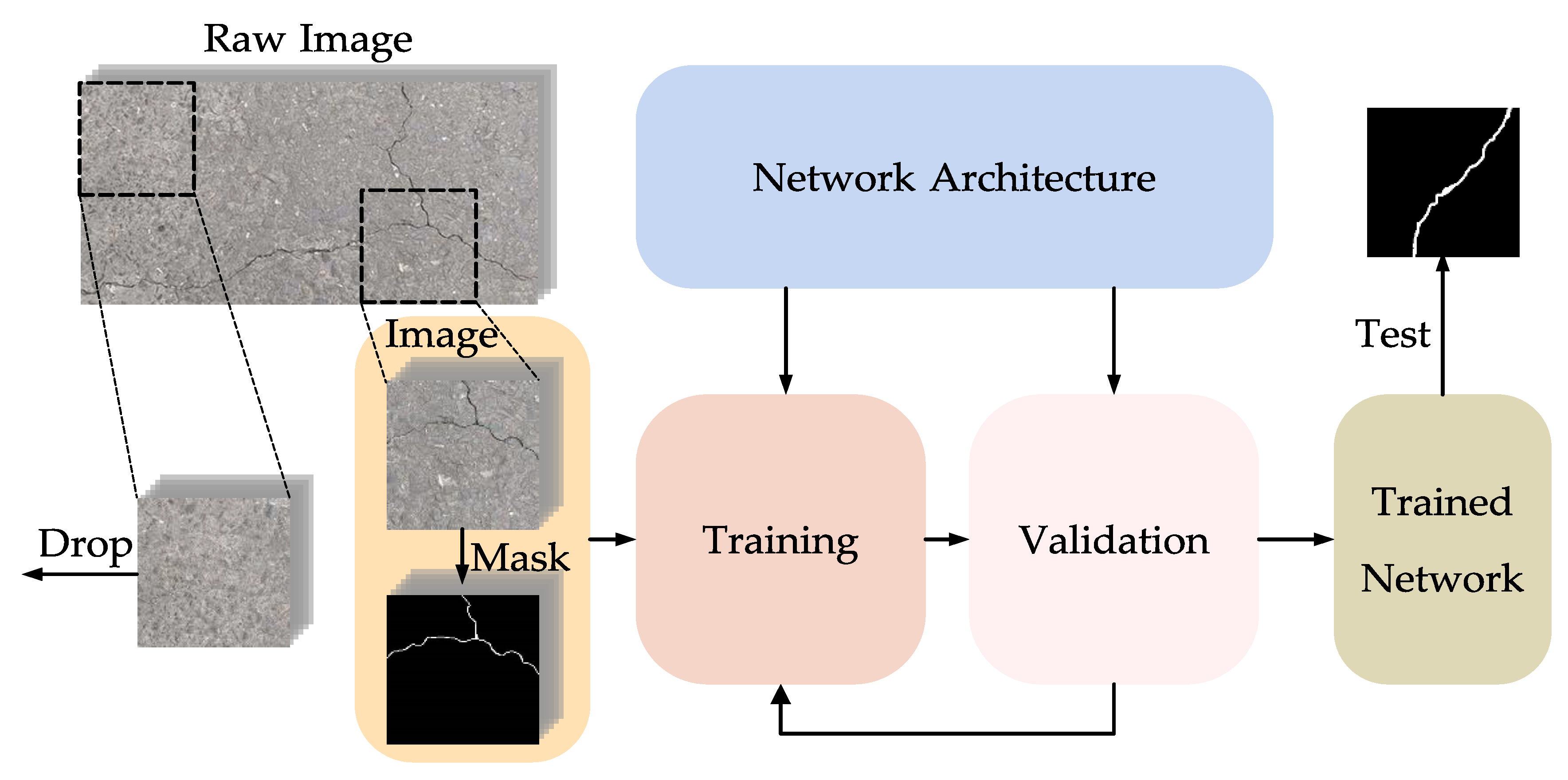
The proposed method achieves the end-to-end crack detection function with a smaller network model and higher segmentation accuracy. To evaluate the effectiveness of the suggested strategy, a concrete crack dataset (CCD) was developed. The process of establishing the CCD is shown in Figure 3. The dataset attempts to encompass all orientations and widths including fractures with simple backgrounds and cracks with complicated backgrounds. The image capture task is carried out using a smartphone. The camera sensor is the IMX600, which is a diagonal 9.2 mm (Type 1/1.7) 40 Mega-pixel CMOS active pixel type stacked image sensor with a square pixel array. The original image is obtained at a resolution of 3648 × 2763, and evenly cropped to 912 × 912. The resolution is reduced to 256 × 256. Image resizing facilitates quick processing. Considering the performance bottleneck of hardware (GPU), 2000 images are carefully selected and labelImgPlus is utilized to make the masks. The network is then trained and validated using the masks and processed images, and the trained network is then used to segment the test images.

3.1. Network

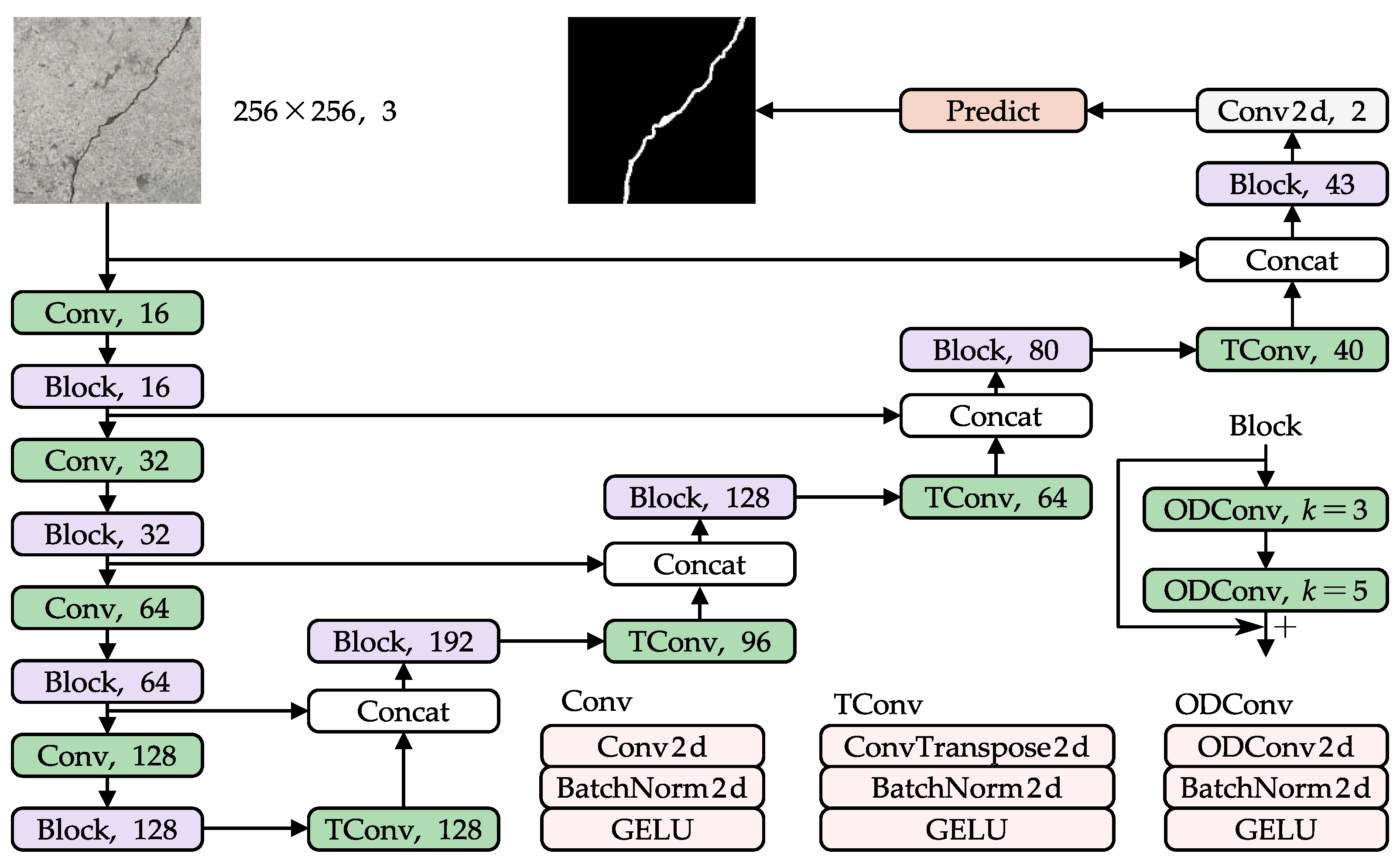
As shown in Figure 4, a pixel-level concrete crack segmentation using pyramidal residual network with Omni-Dimensional Dynamic Convolution is proposed, where the first parameter in the block indicates the block name and the second parameter indicates the number of output filters. The input is an image with a size of 256 × 256 and 3 channels of RGB, and after network calculation the output is a feature map of size 256 × 256 with 2 channels to achieve pixel-level segmentation. These 2 channels correspond to the two classes of crack and background. The network consists of an encoder–decoder. The encoder descending through Conv consist of three parts: convolutional operations, batch normalization (BN), and GELU [48] activation function. The decoder ascending through TConv consists of convolutional operations, BN, and GELU activation function. The block is made of two ODConvs, including three parts: transpose convolutional operations, BN, and GELU activation function. These two blocks are sequentially connected to deepen the network, but they are also Skip Connected to prevent gradients from fading. The feature fusion of the encoder–decoder part is channel concatenating (Concat), and the connection strategy is mentioned later. Network details are tabulated in

Table 1. Detailed parameters in CCSN.

Layer Name	Filter Size	Stride	Output Size	Operational Layers
Input image	-	-	256 × 256 × 3	-
Conv	5 × 5	2	128 × 128 × 16	BN, GELU
ODConv	3 × 3	1	128 × 128 × 8	BN, GELU
ODConv	5 × 5	1	128 × 128 × 16	BN, GELU
ADD	-	-	128 × 128 × 16	-
Conv	5 × 5	2	64 × 64 × 32	BN, GELU
ODConv	3 × 3	1	64 × 64 × 16	BN, GELU
ODConv	5 × 5	1	64 × 64 × 32	BN, GELU
ADD	-	-	64 × 64 × 32	-
Conv	5 × 5	2	32 × 32 × 64	BN, GELU
ODConv	3 × 3	1	32 × 32 × 32	BN, GELU
ODConv	5 × 5	1	32 × 32 × 64	BN, GELU
ADD	-	-	32 × 32 × 64	-
Conv	5 × 5	2	16 × 16 × 128	BN, GELU
ODConv	3 × 3	1	16 × 16 × 64	BN, GELU
ODConv	5 × 5	1	16 × 16 × 128	BN, GELU
ADD	-	-	16 × 16 × 128	-
TConv	4 × 4	2	32 × 32 × 128	BN, GELU
Connecting	-	-	32 × 32 × 192	Concatenation
ODConv	3 × 3	1	32 × 32 × 96	BN, GELU
ODConv	5 × 5	1	32 × 32 × 192	BN, GELU
ADD	-	-	32 × 32 × 192	-
TConv	4 × 4	2	64 × 64 × 96	BN, GELU
Connecting	-	-	64 × 64 × 128	Concatenation
ODConv	3 × 3	1	64 × 64 × 64	BN, GELU
ODConv	5 × 5	1	64 × 64 × 128	BN, GELU
ADD	-	-	64 × 64 × 128	-
TConv	4 × 4	2	128 × 128 × 64	BN, GELU
Connecting	-	-	128 × 128 × 80	Concatenation
ODConv	3 × 3	1	128 × 128 × 40	BN, GELU
ODConv	5 × 5	1	128 × 128 × 80	BN, GELU
ADD	-	-	128 × 128 × 80	-
TConv	4 × 4	2	256 × 256 × 40	BN, GELU
Connecting	-	-	256 × 256 × 43	Concatenation
ODConv	3 × 3	1	256 × 256 × 21	BN, GELU
ODConv	5 × 5	1	256 × 256 × 43	BN, GELU
ADD	-	-	256 × 256 × 43	-
Conv	1 × 1	1	256 × 256 × 2	-
Classification	-	-	256 × 256 × 2	Loss function

.

3.1.1. Conv and TConv Layers

In the method proposed in this paper, Conv is mainly used for reducing the dimensionality of the feature map and changing the number of filters. The kernel size for the convolution operation in Conv is 5 × 5, the stride is set to 2 × 2, and the padding is set to ensure that the size of the resulting feature map is $2^n$. TConv is used to raise the dimensionality and change the number of filters, and the kernel size in TConv is 4 × 4, with other parameters remaining the same as in Conv.

3.1.2. Block

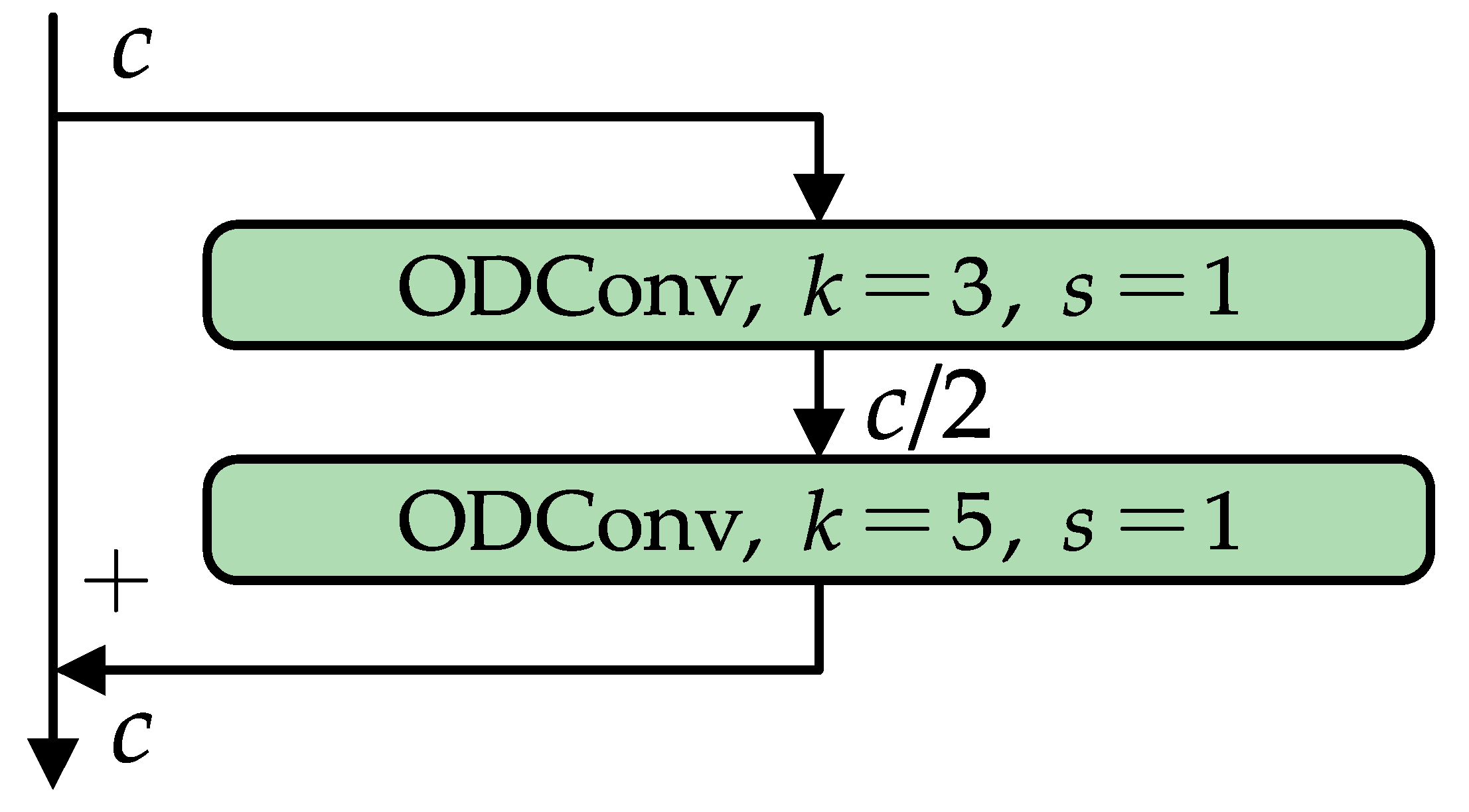
As shown in Figure 5, to solve the degradation problem of deep networks, the block used in this paper adopts the idea of residual blocks. Each block has two convolution operations with different numbers of filters, which can significantly extract two different levels of features in the residual block and accelerate the training process. To find a sense field suitable for crack segmentation and inspired by ConvNeXt [49], the block in this paper attempts to increase the kernel size to improve network performance, which is actually demonstrated by Conv and TConv. However, too large of a kernel size in convolutional operation would entail a huge amount of computation, leading to a trade-off between accuracy and speed. The reasons for choosing convolutional kernel sizes of 3 × 3 and 5 × 5 will be given in the subsequent experimental section.

In Figure 5, $c$ is the number of filters. Assume that the number of filters in the input block is c, and the number of filters will be halved ($c/2$) before the features are restored after entering the block. This method has the advantage of reducing the computation amount and somewhat alleviating the computational load caused by large convolutional kernels.

3.1.3. Connect Strategy

In this study, the feature connection sites during the feature fusion phase are analyzed in depth to further optimize network performance. Under the same assured feature dimensionality, four connection options are experimentally validated, and precise performance is provided in the following experimental section.

3.2. Loss

The cracked dataset is a typical example of an unbalanced class problem; the image contains a disproportionate number of non-cracked pixels and a small number of cracked pixels. To solve this problem, this paper combines focal loss and dice loss, and the loss function can be written in the following form:

$$\mathrm{Loss}=1-{\displaystyle \sum _{c=1}^M{\left(1-p_c\right)}^{\gamma }{y}_c\log p_{\mathrm{c}}}-\frac{2I+\epsilon }{U+\epsilon }$$

(8)

where the first half is the addition of a weighting coefficient ${\left(1-p_t\right)}^{\gamma }$ before the standard cross entropy, and the second half is the dice coefficient. The $\epsilon$ is an artificially set smoothness coefficient, $I$ denotes the intersection of positive examples, and the $U$ denotes the union of examples.

4. Experiments and Results

This section presents the experimental results of the proposed method, including its performance under different network parameters, connection strategies, and losses. At the same time, this network is compared with other networks of the same type. In this paper, to verify the effectiveness of the method, the public crack dataset is selected for further validation.

4.1. Training Configuration

The experiments were conducted using AMD Ryzen7 5800H Processor with 16 GB RAM, and NVIDIA GeForce RTX 3060 Laptop with 6 GB RAM GPU. The DL framework is pytorch, and Adam with a momentum of 0.9 was chosen as the optimizer during training. The initial learning rate and minimum learning rate were set to ${10}^{-4}$ and ${10}^{-6}$, respectively, and the learning rate descent formula is cos. Due to memory constraints, the number of multithreads and batch size were set to 4, and 50 epochs were used for training. The training process was analyzed using different sets of hyperparameters to select the optimal validated model configuration. The dataset was portioned into 80% (1600 images) for training, 10% (200 images) for validation, and 10% (200 images) for testing. All images used in the experiment were set to 256 × 256.

4.2. Evaluation Metric

To evaluate this crack segmentation network, the images were trained with a variety of different parameters, losses, architectures, and networks. Since the crack dataset is a class-imbalanced dataset, if the mean accuracy is simply used as an evaluation metric, the accuracy of the crack pixels will be masked by the accuracy of background pixels and the results will not be well observed. The mIoU is used as the main evaluation metric to assess the performance of the method, and the metrics such as precision (P), recall (R), F1-score, accuracy, and mPA (mean pixel accuracy) are compared. These evaluation metrics can be derived from a confusion matrix. The confusion matrix is shown in

Table 2. The confusion matrix for evaluation.

Pixel		Mask
		Positive	Negative
Predict	Positive	TP	FP
	Negative	FN	TN

.

The evaluation metrics for single class are shown as follows:

$$\mathrm{Precision}=\frac{\mathrm{TP}}{\mathrm{TP}+\mathrm{FP}}$$

(9)

$$\mathrm{Recall}=\frac{\mathrm{TP}}{\mathrm{TP}+\mathrm{FN}}$$

(10)

$$\mathrm{F}1-\mathrm{score}=\frac{2\mathrm{PR}}{\mathrm{P}+\mathrm{R}}$$

(11)

$$\mathrm{IoU}=\frac{\mathrm{TP}}{\mathrm{TP}+\mathrm{FP}+\mathrm{FN}}$$

(12)

$$\mathrm{Accuracy}=\frac{\mathrm{TP}+\mathrm{TN}}{\mathrm{TP}+\mathrm{FP}+\mathrm{FN}+\mathrm{TN}}$$

(13)

The precision indicates the percentage of correctly predicted pixels out of all pixels predicted by the model as positive examples. Recall indicates the percentage of all samples with positive true pixels predicted. mPA indicates the average value of the sum of the precision of all classes. Accuracy indicates the number of correctly predicted pixels as a percentage of all pixels. Moreover, mIoU indicates the summed re-average of all classes of IoU.

4.3. Network Results

4.3.1. Block

For cracked pixels, it has not been investigated how large a window should be used in the feature extraction process to obtain the connection with the surrounding pixels. To find the corresponding parameters suitable for crack segmentation, similar to ConvNeXt with a guaranteed number of parameters, this paper explores the different kernel sizes of the two ODConvs in the block.

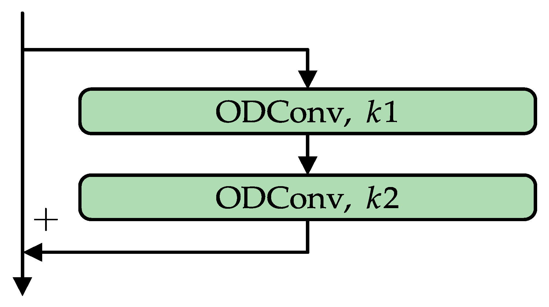
The structure of the block is shown in Figure 6, with the kernel sizes $k1$ and $k2$ set in the order of network connections. To verify the advantages of ODConv and compare the results with the block using normal convolutional operations, the comparison results are shown in

Table 3. Results of different kernel size in block.

k1	k2	ODConv	Accuracy	F1-Score	mIoU	mPA
1	3		0.9897	0.9184	0.8583	0.9143
1	3	√	0.9903	0.9244	0.8675	0.9281
3	5		0.9900	0.9212	0.8626	0.9217
3	5	√	0.9905	0.9261	0.8700	0.9300
5	7		0.9902	0.9229	0.8651	0.9218
5	7	√	0.9904	0.9249	0.8681	0.9294

. It is obvious that $k1$ and $k2$ have better performance when set to 3 and 5, respectively.

To verify the superiority of the method, the blocks in this paper are also compared with ResBlock, MobileNetV3 [50], and ConvNeXt. The experiments were performed in the same environment, but the difference is to replace the blocks with the corresponding methods. The experimental results are shown in

Table 4. Results of different blocks.

Block	Accuracy	F1-Score	mIoU	mPA
ResBlock	0.9900	0.9216	0.8632	0.9254
MobileNetV3	0.9900	0.9199	0.8606	0.9160
ConvNeXt	0.9893	0.9170	0.8561	0.9245
Ours	0.9905	0.9261	0.8700	0.9300

. The method proposed in this paper is notably superior to the alternatives.

4.3.2. Connection Strategy

The feature fusion at different scales of the network is based on the feature pyramid networks. Even for the same network structure, different connection modes may not increase the number of parameters, but they will cause different results. In this paper, four different feature fusion patterns are investigated, as shown in Figure 7. The results in

Table 5. Results of different connection mode.

Mode	Accuracy	F1-Score	mIoU	mPA
b2c	0.9905	0.9261	0.8700	0.9300
b2b	0.9903	0.9241	0.8670	0.9273
c2c	0.9905	0.9259	0.8697	0.9291
c2b	0.9904	0.9247	0.8679	0.9270

show that (a) type of connectivity achieves better results in this method.

4.3.3. Pyramid Structure

The width (channels) of the feature map in the decoder is shown in Figure 8, where the numbers indicate the number of channels. A total of 128 channels were input to the decoder section, and 64, 32, 16, and 3 channels were incorporated into the feature fusion phase from the encoder section when the feature dimension was transformed. The whole network constitutes a feature pyramid. This part obtains the feature pyramid suitable for this network by studying the changing trend of the feature pyramid.

In this paper, the trends of the four feature widths are compared and validated, as shown in

Table 6. Results of different filters.

Width	Accuracy	F1-Score	mIoU	mPA
128, 128, 64, 64	0.9905	0.9251	0.8685	0.9253
128, 64, 32, 16	0.9903	0.9248	0.8680	0.9299
64, 32, 16, 8	0.9901	0.9230	0.8652	0.9287
128, 96, 64, 40	0.9905	0.9261	0.8700	0.9300

, where width indicates the number of channels per TConv output since the features are transmitted along in the direction. The results show that widths of 128, 96, 64, and 40 perform best in this order.

4.4. Loss Results

The loss functions are described in detail in the previous sections. This section examines the performance of different loss functions on our network, as shown in

Table 7. Results of different loss functions.

Mode	Accuracy	F1-Score	mIoU	mPA
CE	0.9905	0.9232	0.8652	0.9101
BCE	0.9905	0.9236	0.8660	0.9143
BCEL	0.9905	0.9231	0.8653	0.9130
IoU	0.9904	0.9224	0.8642	0.9123
Dice	0.9903	0.9246	0.8677	0.9285
FL	0.9904	0.9228	0.8647	0.9111
OhemCE	0.9905	0.9234	0.8657	0.9123
Ours	0.9905	0.9261	0.8700	0.9300

. The results show that this method, which uses focal loss and takes into account the dice coefficient, outperforms other loss functions.

4.5. Other Network Results

4.5.1. Results on CCD

To validate the effectiveness of the proposed method, the method in this paper is compared with other methods, including classical algorithms FCN, SegNet, Unet, and Deeplabv3+. In addition, the method is compared with Swin-unet using pure transformer, which further demonstrates its advantages in crack segmentation task.

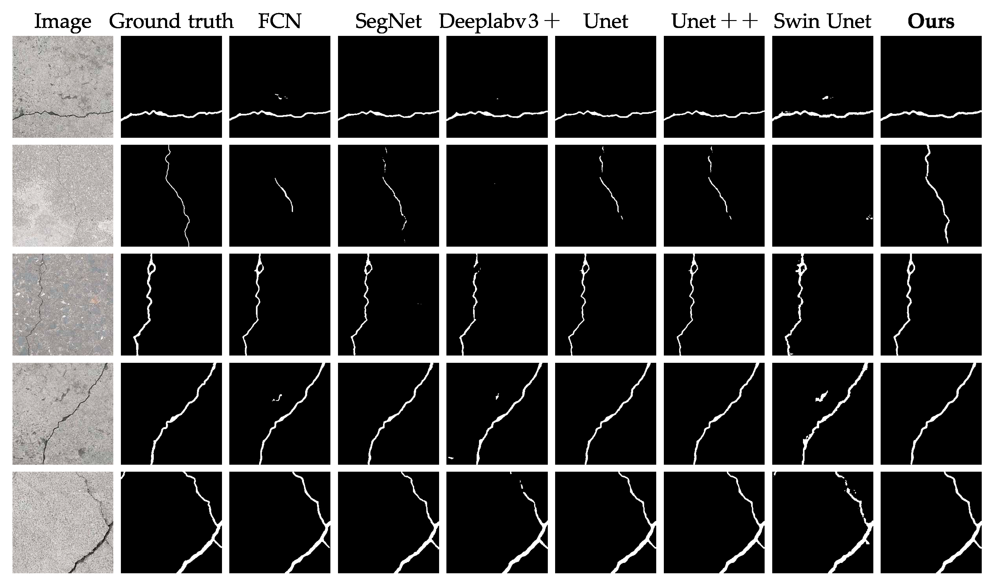
The experimental results are shown in

Table 8. Results of different networks by CCD.

Mode	Accuracy	F1-Score	mIoU	mPA
FCN	0.9894	0.9137	0.8508	0.8977
SegNet	0.9895	0.9137	0.8506	0.8951
Deeplabv3+	0.9861	0.8827	0.8052	0.8511
Unet	0.9898	0.9169	0.8556	0.9025
Unet++	0.9901	0.9203	0.8609	0.9092
Swin-unet	0.9860	0.8907	0.8184	0.8944
CCSN (Ours)	0.9905	0.9261	0.8700	0.9300

, where the U-shaped network and the coder–decoder structure crack segmentation task exhibit better performances, while algorithms such as Deeplabv3+ and Swin-unet show disappointing performances. The method proposed in this paper outperforms other methods in terms of accuracy, F1-score, mIoU, and mPA. Samples of crack detection using different networks are shown in Figure 9. In the second test sample, for example, fine (only one pixel wide) and blurred cracks pose a challenge to detection, but our method is able to detect the whole crack more completely and comes closest to the truth image of the ground.

4.5.2. Results on BCL Dataset

To enhance the persuasiveness of the methods in this paper, the Bridge Crack Library (BCL) [51] dataset published on Harvard Dataverse in 2020 was used to validate the mentioned network, as shown in

Table 9. Results of different networks by BCL.

Mode	Accuracy	F1-Score	mIoU	mPA
FCN	0.9875	0.8697	0.7902	0.8517
SegNet	0.9884	0.8802	0.8042	0.8659
Deeplabv3+	0.9875	0.8721	0.7938	0.8616
Unet	0.9884	0.8822	0.8072	0.8743
Unet++	0.9874	0.8617	0.7766	0.8193
Swin-unet	0.9853	0.8590	0.7767	0.8736
CCSN (Ours)	0.9889	0.8925	0.8209	0.9047

. In a random sample of 2000 images from the BCL dataset, 80% of them were used for training, 10% for validation, and 10% for testing, so as to ensure that the same environment as the CCD is used to start the experiments. The experimental results show that the proposed method in this paper achieves an accuracy of 98.89%, mIoU of 82.9%, and mPA of 90.47% on the BCL dataset, which are higher than other networks.

4.6. Computational Comparison

The computational complexity of the proposed CCSN network was evaluated against other networks (FCN, SegNet, DeepLabv3+, Unet, Unet++, Swin-unet). The actual performance of this method was evaluated by comparing the number of parameters, floating point operations (FLOPs), memory storage, and FPS comparisons of these networks. The computational complexity is shown in

Table 10. Computational comparison of CCSN and other networks.

Mode	Param (M)	FLOPs (G)	Storage (MB)	Training Time (min)	FPS
FCN	120.48	806.55	114	382.33	9.37
SegNet	117.78	40.08	112	68.12	65.53
Deeplabv3+	208.43	20.66	208	78.05	40.43
Unet	128.36	50.70	122	89.50	50.90
Unet++	188.78	200.11	180	214.95	17.17
Swin-unet	108.58	76.90	105	54.88	48.68
CCSN(Ours)	4.28	7.17	9.61	65.67	43.04

. For all networks including training datasets, test datasets, and hyperparameters, the network training criteria were set identically. The proposed CCSN network consists of 4.28 million learnable parameters, with only 7.17 GFLOPs and 9.61 MB storage, all of which are much lower than other networks. In addition, the training time of this method in the experiment is 65.67 min, which is shorter among all methods. In terms of FPS, the proposed network in this paper outperforms DeepLabv3+ and Unet++, and is slightly lower than SegNet, Unet, and Swin-unet. However, its overall evaluation metrics are still greatly dominated.

5. Conclusions

In this study, a crack segmentation network for automatic pixel-level crack detection is designed and implemented. Firstly, the network parameters and structure are investigated in detail so as to discover an appropriate network window size, feature connection strategy, and dimensional transformation method for crack segmentation. Then, to solve the class imbalance problem, focal loss is integrated with the dice coefficient to improve the overall accuracy of the method. To evaluate the performance, a new crack dataset (CCD) is used for training and validation. The training process is examined on the validation images, with an average accuracy of 99.05%, mIoU of 87.00%, and mPA of 93.00%. In addition, training and validation on the public dataset (BCL) also outperformed the other networks in terms of overall performance. This work provides not only further prospects for improving the accuracy of crack segmentation but also a reference for subsequent related research. The next step is to deploy the method to a wall-climbing robot or UAV for further validation and fine-tuning to adapt to the actual inspection environment.

References

1. Lu, L.; Ouyang, D. Properties of Cement Mortar and Ultra-High Strength Concrete Incorporating Graphene Oxide Nanosheets. Nanomaterials 2017, 7, 187. [Google Scholar] [CrossRef]
2. Adhikari, R.S.; Moselhi, O.; Bagchi, A. Image-based retrieval of concrete crack properties for bridge inspection. Autom. Constr. 2014, 39, 180–194. [Google Scholar] [CrossRef]
3. Rein-Lien, H.; Abdel-Mottaleb, M.; Jain, A.K. Face detection in color images. IEEE Trans. Pattern Anal. Mach. Intell. 2002, 24, 696–706. [Google Scholar] [CrossRef]
4. Abanto-Bueno, J.; Lambros, J. Investigation of crack growth in functionally graded materials using digital image correlation. Eng. Fract. Mech. 2002, 69, 1695–1711. [Google Scholar] [CrossRef]
5. Eshera, M.A.; Fu, K.-S. A graph distance measure for image analysis. IEEE Trans. Syst. Man, Cybern. 1984, SMC-14, 398–408. [Google Scholar] [CrossRef]
6. Tang, Y.; Zhu, M.; Chen, Z.; Wu, C.; Chen, B.; Li, C.; Li, L. Seismic performance evaluation of recycled aggregate concrete-filled steel tubular columns with field strain detected via a novel mark-free vision method. Structures 2022, 37, 426–441. [Google Scholar] [CrossRef]
7. Chen, X.; Wu, H.; Lichti, D.; Han, X.; Ban, Y.; Li, P.; Deng, H. Extraction of indoor objects based on the exponential function density clustering model. Inf. Sci. 2022, 607, 1111–1135. [Google Scholar] [CrossRef]
8. Lei, B.; Wang, N.; Xu, P.; Song, G. New Crack Detection Method for Bridge Inspection Using UAV Incorporating Image Processing. J. Aerosp. Eng. 2018, 31. [Google Scholar] [CrossRef]
9. Liu, Q.; Liu, Y. An approach for auto bridge inspection based on climbing robot. In Proceedings of the 2013 IEEE International Conference on Robotics and Biomimetics (ROBIO), Shenzhen, China, 12–14 December 2013. [Google Scholar]
10. Young, T.; Hazarika, D.; Poria, S.; Cambria, E. Recent Trends in Deep Learning Based Natural Language Processing. IEEE Comput. Intell. Mag. 2018, 13, 55–75. [Google Scholar] [CrossRef]
11. Mandal, V.; Uong, L.; Adu-Gyamfi, Y. Automated road crack detection using deep convolutional neural networks. In Proceedings of the 2018 IEEE International Conference on Big Data (Big Data), Seattle, WA, USA, 10–13 December 2018. [Google Scholar]
12. Cha, Y.-J.; Choi, W.; Büyüköztürk, O. Deep Learning-Based Crack Damage Detection Using Convolutional Neural Networks. Comput. Civil Infrastruct. Eng. 2017, 32, 361–378. [Google Scholar] [CrossRef]
13. Lee, D.; Kim, J.; Lee, D. Robust Concrete Crack Detection Using Deep Learning-Based Semantic Segmentation. Int. J. Aeronaut. Space Sci. 2019, 20, 287–299. [Google Scholar] [CrossRef]
14. Que, Y.; Dai, Y.; Ji, X.; Leung, A.K.; Chen, Z.; Jiang, Z.; Tang, Y. Automatic classification of asphalt pavement cracks using a novel integrated generative adversarial networks and improved VGG model. Eng. Struct. 2023, 277, 115406. [Google Scholar] [CrossRef]
15. Tang, Y.; Huang, Z.; Chen, Z.; Chen, M.; Zhou, H.; Zhang, H.; Sun, J. Novel visual crack width measurement based on backbone double-scale features for improved detection automation. Eng. Struct. 2023, 274, 115158. [Google Scholar] [CrossRef]
16. Jin, X.; Haider, M.Z.; Cui, Y.; Jang, J.G.; Kim, Y.J.; Fang, G.; Hu, J.W. Development of nanomodified self-healing mortar and a U-Net model based on semantic segmentation for crack detection and evaluation. Constr. Build. Mater. 2023, 365, 129985. [Google Scholar] [CrossRef]
17. Shelhamer, E.; Long, J.; Darrell, T. Fully convolutional networks for semantic segmentation. IEEE Trans. Pattern Anal. Mach. Intell. 2017, 39, 640–651. [Google Scholar] [CrossRef]
18. Ronneberger, O.; Fischer, P.; Brox, T. U-Net: Convolutional Networks for Biomedical Image Segmentation. In Medical Image Computing and Computer-Assisted Intervention—MICCAI 2015; Navab, N., Hornegger, J., Wells, W.M., Frangi, A.F., Eds.; Springer International Publishing: Cham, Switzerland, 2015; pp. 234–241. [Google Scholar]
19. Badrinarayanan, V.; Kendall, A.; Cipolla, R. Segnet: A deep convolutional encoder-decoder architecture for image segmentation. IEEE Trans. Pattern Anal. Mach. Intell. 2017, 39, 2481–2495. [Google Scholar] [CrossRef]
20. Yu, F.; Koltun, V. Multi-scale context aggregation by dilated convolutions. arXiv Preprint 2015, arXiv:1511.07122. [Google Scholar]
21. Chen, L.-C.; Papandreou, G.; Kokkinos, I.; Murphy, K.; Yuille, A.L. Semantic Image Segmentation with Deep Convolutional Nets and Fully Connected CRFs. arXiv 2014, arXiv:1412.7062. [Google Scholar]
22. Chen, L.-C.; Papandreou, G.; Kokkinos, I.; Murphy, K.; Yuille, A.L. DeepLab: Semantic Image Segmentation with Deep Convolutional Nets, Atrous Convolution, and Fully Connected CRFs. IEEE Trans. Pattern Anal. Mach. Intell. 2018, 40, 834–848. [Google Scholar] [CrossRef] [PubMed]
23. Chen, L.-C.; Papandreou, G.; Schroff, F.; Adam, H. Rethinking Atrous Convolution for Semantic Image Segmentation. arXiv 2017, arXiv:1706.05587. [Google Scholar]
24. Chen, L.-C.; Zhu, Y.; Papandreou, G.; Schroff, F.; Adam, H. In Encoder-decoder with atrous separable convolution for semantic image segmentation. In Proceedings of the European Conference on Computer Vision (ECCV) 2018, Munich, Germany, 8–14 September 2018; pp. 801–818. [Google Scholar]
25. Yang, M.; Yu, K.; Zhang, C.; Li, Z.; Yang, K. DenseASPP for Semantic Segmentation in Street Scenes. In Proceedings of the 2018 IEEE/CVF Conference on Computer Vision and Pattern Recognition, Salt Lake City, UT, USA, 18–23 June 2018. [Google Scholar]
26. Peng, C.; Zhang, X.; Yu, G.; Luo, G.; Sun, J. Large Kernel Matters—Improve Semantic Segmentation by Global Convolutional Network. In Proceedings of the 2017 IEEE Conference on Computer Vision and Pattern Recognition (CVPR), Honolulu, HI, USA, 21–26 July 2017; pp. 4353–4361. [Google Scholar] [CrossRef]
27. Zhao, H.; Shi, J.; Qi, X.; Wang, X.; Jia, J. In Pyramid scene parsing network. In Proceedings of the IEEE Conference on Computer Vision and Pattern Recognition 2017, Honolulu, HI, USA, 21–26 July 2017; pp. 2881–2890. [Google Scholar]
28. Cao, H.; Wang, Y.; Chen, J.; Jiang, D.; Zhang, X.; Tian, Q.; Wang, M. Swin-unet: Unet-like pure transformer for medical image segmentation. arXiv Preprint 2021, arXiv:2105.05537. [Google Scholar]
29. Carr, T.A.; Jenkins, M.D.; Iglesias, M.I.; Buggy, T.; Morison, G. Road crack detection using a single stage detector based deep neural network. In Proceedings of the 2018 IEEE Workshop on Environmental, Energy, and Structural Monitoring Systems (EESMS), Salerno, Italy, 21–22 June 2018. [Google Scholar] [CrossRef]
30. Yang, F.; Zhang, L.; Yu, S.; Prokhorov, D.; Mei, X.; Ling, H. Feature Pyramid and Hierarchical Boosting Network for Pavement Crack Detection. arXiv 2019, arXiv:1901.06340. [Google Scholar] [CrossRef] [Green Version]
31. Jiang, W.; Liu, M.; Peng, Y.; Wu, L.; Wang, Y. HDCB-Net: A Neural Network with the Hybrid Dilated Convolution for Pixel-Level Crack Detection on Concrete Bridges. IEEE Trans. Ind. Informat. 2020, 17, 5485–5494. [Google Scholar] [CrossRef]
32. Cheng, J.; Xiong, W.; Chen, W.; Gu, Y.; Li, Y. Pixel-level Crack Detection using U-Net. In Proceedings of the TENCON 2018—2018 IEEE Region 10 Conference, Jeju, Republic of Korea, 28–31 October 2018. [Google Scholar]
33. Ji, J.; Wu, L.; Chen, Z.; Yu, J.; Lin, P.; Cheng, S. Automated Pixel-Level Surface Crack Detection Using U-Net. In Multi-Disciplinary Trends in Artificial Intelligence; Kaenampornpan, M., Malaka, R., Nguyen, D.D., Schwind, N., Eds.; Springer International Publishing: Cham, Switzerland, 2018; pp. 69–78. [Google Scholar] [CrossRef]
34. Leal da Silva, W.R.; Schwerz de Lucena, D. Concrete Cracks Detection Based on Deep Learning Image Classification. Proceedings 2018, 2, 489. [Google Scholar]
35. Zou, Q.; Zhang, Z.; Li, Q.; Qi, X.; Wang, Q.; Wang, S. DeepCrack: Learning Hierarchical Convolutional Features for Crack Detection. IEEE Trans. Image Process. 2018, 28, 1498–1512. [Google Scholar] [CrossRef] [PubMed]
36. Liu, Z.; Cao, Y.; Wang, Y.; Wang, W. Computer vision-based concrete crack detection using U-net fully convolutional networks. Autom. Constr. 2019, 104, 129–139. [Google Scholar] [CrossRef]
37. Zhang, X.; Rajan, D.; Story, B. Concrete crack detection using context-aware deep semantic segmentation network. Comput. Civ. Infrastruct. Eng. 2019, 34, 951–971. [Google Scholar] [CrossRef]
38. Liu, Y.; Yao, J.; Lu, X.; Xie, R.; Li, L. DeepCrack: A deep hierarchical feature learning architecture for crack segmentation. Neurocomputing 2019, 338, 139–153. [Google Scholar] [CrossRef]
39. Sudre, C.H.; Li, W.; Vercauteren, T.; Ourselin, S.; Jorge Cardoso, M. In Generalised Dice Overlap as a Deep Learning Loss Function for Highly Unbalanced Segmentations. In Deep Learning in Medical Image Analysis and Multimodal Learning for Clinical Decision Support; Cardoso, M.J., Arbel, T., Carneiro, G., Syeda-Mahmood, T., Tavares, J.M.R.S., Moradi, M., Bradley, A., Greenspan, H., Papa, J.P., Madabhushi, A., Eds.; Springer International Publishing: Cham, Switzerland, 2017; pp. 240–248. [Google Scholar]
40. Lin, T.-Y.; Goyal, P.; Girshick, R.; He, K.; Dollar, P. Focal Loss for Dense Object Detection. IEEE Trans. Pattern Anal. Mach. Intell. 2020, 42, 318–327. [Google Scholar] [CrossRef] [Green Version]
41. He, K.; Zhang, X.; Ren, S.; Sun, J. Deep Residual Learning for Image Recognition. In Proceedings of the 2016 IEEE Conference on Computer Vision and Pattern Recognition (CVPR), Las Vegas, NV, USA, 27–30 June 2016. [Google Scholar]
42. Li, C.; Zhou, A.; Yao, A. Omni-Dimensional Dynamic Convolution. arXiv 2022, arXiv:2209.07947. [Google Scholar]
43. Hu, J.; Shen, L.; Sun, G. Squeeze-and-Excitation Networks. In Proceedings of the 2018 IEEE/CVF Conference on Computer Vision and Pattern Recognition, Salt Lake City, UT, USA, 18–23 June 2018. [Google Scholar]
44. Han, D.; Kim, J.; Kim, J. Deep Pyramidal Residual Networks. In Proceedings of the 2017 IEEE Conference on Computer Vision and Pattern Recognition (CVPR), Honolulu, HI, USA, 21–26 June 2017. [Google Scholar]
45. Lin, T.-Y.; Dollar, P.; Girshick, R.; He, K.; Hariharan, B.; Belongie, S. Feature Pyramid Networks for Object Detection. In Proceedings of the 2017 IEEE Conference on Computer Vision and Pattern Recognition (CVPR), Honolulu, HI, USA, 21–26 June 2017. [Google Scholar]
46. Shrivastava, A.; Gupta, A.; Girshick, R. Training Region-Based Object Detectors with Online Hard Example Mining. In Proceedings of the 2016 IEEE Conference on Computer Vision and Pattern Recognition (CVPR), Las Vegas, NV, USA, 27–30 June 2016. [Google Scholar]
47. Milletari, F.; Navab, N.; Ahmadi, S.-A. V-net: Fully convolutional neural networks for volumetric medical image segmentation. In Proceedings of the 2016 Fourth International Conference on 3D Vision (3DV), Stanford, CA, USA, 25–28 October 2016. [Google Scholar]
48. Hendrycks, D.; Gimpel, K. Bridging nonlinearities and stochastic regularizers with gaussian error linear units. In Proceedings of the ICLR 2017 Conference, Toulon, France, 24–26 April 2017. [Google Scholar]
49. Liu, Z.; Mao, H.; Wu, C.-Y.; Feichtenhofer, C.; Darrell, T.; Xie, S. A ConvNet for the 2020s. In Proceedings of the 2022 IEEE/CVF Conference on Computer Vision and Pattern Recognition (CVPR), New Orleans, LA, USA, 19–20 June 2022. [Google Scholar]
50. Howard, A.; Sandler, M.; Chen, B.; Wang, W.; Chen, L.-C.; Tan, M.; Chu, G.; Vasudevan, V.; Zhu, Y.; Pang, R.; et al. Searching for MobileNetV3. In Proceedings of the 2019 IEEE/CVF International Conference on Computer Vision (ICCV), Seoul, Republic of Korea, 27 October–2 November 2019. [Google Scholar]
51. Jin, T.; Li, Z.; Ding, Y.; Ma, S.; Ou, Y. Bridge Crack Library. In V1, Deaccessioned Version ed.; Harvard Dataverse, 2020. Available online: https://dataverse.harvard.edu/dataset.xhtml?persistentId=doi:10.7910/DVN/RURXSH (accessed on 17 November 2022).
Figure 1. Inference mIoU, FLOPs, speed, and storage performance on our dataset. The bigger the circle, the faster the speed. The redder the color, the larger the storage.
Processes 11 00546 g001
Figure 2. A schematic of ODConv uses GAP + FC + Sigmoid.
Processes 11 00546 g002
Figure 3. Overview of the proposed segmentation framework.
Processes 11 00546 g003
Figure 4. Schematic illustration of CCSN network architecture.
Processes 11 00546 g004
Figure 5. Schematic illustration of Block.
Processes 11 00546 g005
Figure 6. Schematic illustration of block with different kernels.
Processes 11 00546 g006
Figure 7. Schematic illustration of different connection mode.
Processes 11 00546 g007
Figure 8. Schematic illustration of decoder feature width.
Processes 11 00546 g008
Figure 9. Samples of crack detection using different networks.
Processes 11 00546 g009