Development of Anomaly Detectors for HVAC Systems Using Machine Learning

Abstract

Faults and anomalous behavior affect the operation of Heating, Ventilation and Air Conditioning (HVAC) systems. This causes performance loss, energy waste, noncompliance with regulations and discomfort among occupants. To prevent damage, automated, fast identification of faults in HVAC systems is needed. Fault Detection and Diagnosis (FDD) techniques are very effective for these purposes. The best FDD methods, in terms of cost effectiveness and data exploitation, are based on process history; i.e., on sensor data from automation systems. In this work, supervised and semi-supervised models were developed. Other than with regard to outdoor temperature and humidity, the input parameters of an HVAC system have few internal variables. Performance of traditional methods (e.g., VAR, Random Forest) is low, so Artificial Neural Networks (ANNs) were selected, since they can capture nonlinear relationships among features and are easily optimized. ANNs can detect simultaneous faults from different classes. ANN metrics are easily evaluated. The ground truth is obtained from process history (supervised case) and from a mix of deterministic methods and clustering (semi-supervised case). The derivation of the ground truth in the semi-supervised case, and extensive comparison with advanced supervised models, set this work apart from previous studies. The Mean Absolute Error (MAE) of the best supervised model was 0.032 over 15 min and 0.034 over 30 min. The Balanced Accuracy Score (BAS) of the best semi-supervised model was 86%.

1. Introduction

Construction and operation of buildings accounted for 36% of worldwide energy demand and for 37% of energy-related ${\mathrm{CO}}_2$ emissions in 2020 [1]. As per the impact assessment for the Climate Target Plan 2030, residential and services buildings should reduce their GHG emissions by 60%, compared to 2015 [2]. Previous studies show that buildings can use 20–40% less energy if poor HVAC control strategies are detected and improved and if more up-to-date HVAC controllers are developed [3,4,5]. To curb energy consumption, some buildings, especially the most modern and large ones, feature automation systems, such as Building Management Systems (BMSs), which monitor and control the HVAC, mechanical and electrical equipment. HVAC systems usually account for 40% of the energy used in buildings [6], and if lighting is included, this figure can reach 70% [7]. The recast Energy Performance of Buildings Directive (EPBD) [8] has spurred on the installation of services, such as building automation, smart meters and control systems, that can ensure high energy savings. Collecting, monitoring and processing HVAC data through the above services helps to detect potential sources of energy waste and faults using FDD techniques, namely, analytical tools enabling the detection of faults in HVAC systems and which provide useful information to plan troubleshooting strategies. Faulty HVAC components account for no less than 30% of the energy used in commercial buildings [9] and this share can be reduced using FDD.

According to Kim and Katipamula [9] FDD methods for building systems can be based (1) on qualitative models, such as rules or qualitative physics; (2) on quantitative models, such as detailed or simplified physical models; and (3) on process history. Quantitative models use algebraic and differential equations that describe the behavior of the systems. Differences between actual measurements and results of these models mark faults. However, solving the underlying equations often requires much effort. HVAC processes are always multivariable, and nonlinear, and involve complex heat and mass transfer. Moreover, validating quantitative models requires detailed experimental data about the building physics and the setup of each system. This makes building quantitative models and using them time-consuming. Quantitative models are very useful for retrofit analysis or for defining renovation strategies [10].

Qualitative models build sets of rules or qualitative equations on a priori knowledge of the systems under study. In rule-based techniques, thresholds are derived by analyzing monitoring data. Qualitative models can be used for real-time control; e.g., for model predictive control [11,12]. They are simple and easy to develop and use. However, they are often tailored to a given system or process, so they are hard to apply to other systems or processes.

Methods based on process history tap the vast amount of sensor data from automation systems, such as BMSs. These methods are cost-effective and can achieve accurate, real-time control of the building systems without in-depth knowledge of the physics of the system or process. Unlike previous models, methods based on process history are highly dependent on the quality of the data provided. Similarly to qualitative models, methods based on process history are often hard to apply outside the data range used to build them.

As quantitative and qualitative models were not viable here, methods based on process history were examined instead. They often rely on supervised learning models (classification for discrete predictors, regression for continuous ones); in other words, they often rely on models requiring labeled data. Methods based on process history can also use unsupervised learning models (e.g., clustering, dimensionality reduction, association rules), these being models using unlabeled data. However, evaluating the performance of these models is case-dependent; thus, they were ignored here.

A labeled dataset is a set of structured data consisting of input and output variables. The latter are termed “label” or “labeled data”. The label can be binary for fault detection and binary fault diagnosis (i.e., whether a data sample is normal or faulty) or multiclass for multiclass fault diagnosis (i.e., whether a data sample marks different health states of a machine or process; e.g., normal, faulty or recovering operation in the case of three classes).

A key challenge in developing methods based on process history is the lack of labeled data, due to the fact that labeling often requires human experts and so collecting enough labeled data to classify faults is time- and resource-consuming. Moreover, samples could be incorrectly labeled [13]. Supervised learning-based FDD of HVAC systems use the following: Support Vector Machines (SVMs) [14,15,16], decision trees [15,16], gradient boosted trees [14,17], random forests [14,16,17], shallow neural networks [15], deep feedforward neural networks [15,18], Recurrent Neural Networks (RNNs) [17,19]. Zhou et al. [15] compared the performance of SVMs, decision trees, clustering (unsupervised method), shallow and deep neural networks to diagnose faults in a variable refrigerant flow system. The SVM model proved to be the best for diagnosing single faults (here, the training dataset included only one fault class), while deep neural networks excelled at diagnosing multiple faults (here, the training dataset included several fault classes). The dynamics of the system and faults related to it were neglected.

Shahnazari et al. [19] used RNNs. Their method could isolate faults in HVAC systems without the need for plant fault history, mechanistic models or expert rules. However, performance was not extensively compared among different RNNs.

Mirnaghi and Haghighat [13] noted that supervised learning-based FDD of HVAC systems was more suitable for steady-state conditions than transient ones. Moreover, they noted that FDD should neglect faulty samples from older HVAC components, as well as the first months or year of operation of HVAC components. This helps in selecting proper case studies.

Available datasets of building systems often include a small amount of labeled data and a large amount of unlabeled data. Semi-supervised learning models can leverage such datasets. Moreover, supervised learning models can seldom identify novel faults [13], unlike semi-supervised learning models. Dey et al. [20] used SVM to classify normal and faulty patterns in a terminal unit of an HVAC system. The SVM was trained on historical (i.e., labeled) data. The SVM models outperformed k-NN classifiers trained and tested on the same data.

To tackle the imbalanced training data problem for AHU FDD (i.e., datasets including a large amount of normal samples and a small amount of anomalies) Yan et al. [21] developed a semi-supervised method using SVM as the base classifier. Samples with confidence levels (classification probabilities) higher than a threshold were pseudo-labeled and added to the training dataset to improve the SVM performance at the next training iteration. The proposed method outperformed existing semi-supervised methods.

Fan et al. [22] and Fan et al. [23] used the same dataset as Yan et al. [21] and adopted a similar approach using three-layer neural networks for both fault diagnosis (16-class classification task) and unseen fault detection. Unseen (unknown) faults are those which are not in training datasets. Many combinations of semi-supervised learning parameters, these being the number of labeled data (per class), minimum confidence score for pseudo-labeling, learning rate, and maximum number of model updates, were examined. To better detect unseen faults, large confidence thresholds and learning rates were suggested.

Elnour et al. [24] developed and validated a semi-supervised attack detection method based on isolation forests for a simulated multi-zone HVAC system.

Li et al. [25] addressed the problem of data scarcity using semi-generative adversarial networks (GANs). However, the proposed method could not diagnose unknown faults in the examined system. Moreover, two different types of faults occurring simultaneously could not be diagnosed.

Martinez-Viol et al. [26] developed a parameter transfer learning approach, in which a reference classifier was trained on data from the source domain and the weights and biases of the reference classifier were used to initialize the classifier for the target domain. The target domain was trained on target data resembling source data. This study proved that transfer learning in HVAC FDD tasks required a high degree of similarity between source and target domains.

Albayati et al. [27] used data collected from a rooftop HVAC unit under normal operating conditions. Five classes of faults were analyzed. Multiple faults could occur at once. Two semi-supervised models were developed: model 1 used SVM as the supervised method, and k-NN labeling as the unsupervised method; model 2 used SVM as the supervised method, and clustering as the unsupervised method. These models classified the minority class in imbalanced datasets more accurately than the supervised model used as baseline. However, the datasets were small: datasets 1 and 2 included 3336 and 2099 samples, respectively. Thus, the applicability of the developed semi-supervised models on larger datasets was not assessed.

Mirnaghi and Haghighat [13] noted that semi-supervised learning-based FDD of HVAC systems required adjusting hyperparameters to different setups of the systems. This type of FDD also required a large amount of normal operation data, which needed to be available beforehand. Overall, semi-supervised learning-based FDD calls for more automation and enough monitored variables to fully define the operating status of the system.

Key Objectives

This work aimed to develop two types of models that perform FDD of proven, well run-in HVAC systems in non-residential buildings:

1.

predictive models that can forecast transient states;

2.

classification models that can be trained on partially labeled datasets with a small number of variables.

These models should be:

• highly accurate in terms of common ML metrics; and
• easily applicable without extensive feature engineering.

2. Materials and Methods

2.1. Case Study Building

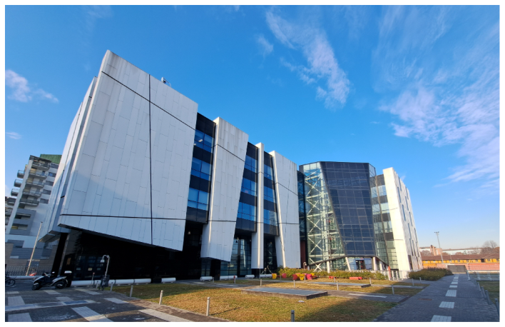
The case study building was the Energy Center, an office building in Turin, Italy (see Figure 1). This building is described in Becchio et al. [28] and Di Già and Papurello [29]. It has five floors, including a basement. The basement houses car parking, laboratories and technical rooms. The first floor houses an exposition hall, which runs through all four above-ground floors, an auditorium and a research laboratory. From the second to the fourth floor, the building houses offices and meeting rooms for companies and start-ups. The following two energy vectors cover most of the energy demand of the building: (1) electricity, through the connection to the medium-voltage grid; and (2) heat, through the connection to the district heating network of Turin. The building is equipped with HVAC systems and with a BMS that controls and manages the entire facility and its equipment.

2.2. Case Study AHU

AHUs bring in outdoor air, control its parameters and feed it to the building’s ductwork for distribution. The controlled parameters are variables, such as temperature, humidity, speed and quality, that ensure the air supplied provides thermo-hygrometric comfort in the room, according to standards such as ISO 7730:2005 [30], EN 16798-1:2019 [31] and ASHRAE 55-2020 [32]. Five all-air recirculating, modular AHUs condition indoor air in the Energy Center. The AHUs monitor the concentration of pollutants in the return air to condition room air and ensure it meets air quality standards. The flow rate of supply air is varied based on Volatile Organic Compounds (VOCs) in the return air, which is partially replaced by outdoor air to replenish oxygen and to remove pollutants and carbon dioxide. The remaining return air is mixed with fresh air and recirculated to reduce energy consumption. Each AHU independently controls one of the following thermal zones:

1.

laboratories (basement);

2.

lobby (from ground floor to third floor);

3.

auditorium (ground floor);

4.

offices (first, second and third floors).

More specifically,

1.

a terminal reheat/cooling AHU in the basement serves the laboratories;

2.

a terminal reheat/cooling AHU in the basement serves the lobby;

3.

a terminal reheat/cooling AHU on the roof serves offices in the northwest wing;

4.

a terminal reheat/cooling AHU on the roof serves offices in the northeast wing;

5.

a single-zone AHU on the roof serves the auditorium.

Single-zone and terminal reheat/cooling AHUs are defined in Seyam [33]. The single-zone AHUs supply the required sensible and latent heating/cooling load to ensure local thermal comfort. The terminal reheat/cooling AHUs supply the required latent heating/cooling load and most of the sensible heating/cooling load. The zone terminal units, such as ceiling radiant panels, supply the remaining part of the sensible heating/cooling load to ensure local thermal comfort.

The AHU serving offices in the northeast wing was analyzed here. It provides the most consistent and complete monitoring data among all AHUs. This AHU conditions air on all three floors of the office area, in both winter and summer.

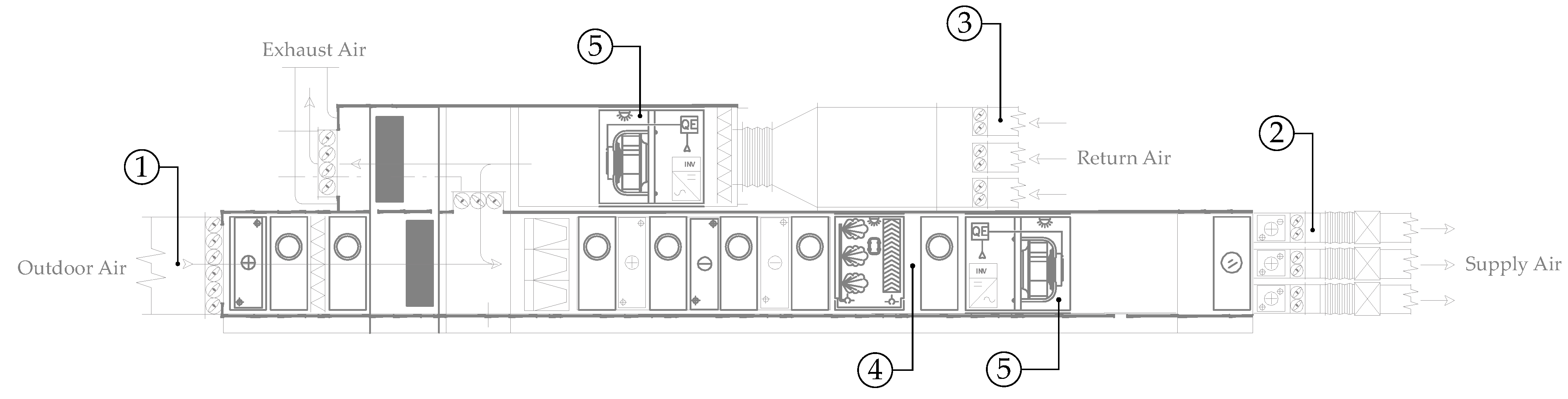
Figure 2 shows the front section of the AHU serving offices in the northeast wing.

Understanding the AHU’s winter operation helped to do the following:

• assign a different importance to each feature in the dataset;
• interpret FDD results;
• perform inspection and maintenance only if need be;
• set physics-based thresholds for confirming or rejecting anomalies identified by data-driven FDD methods; and
• focus on a specific stage of the AHU between two or more sensors.

2.3. Dataset

AHU monitoring data, see Section 2.2, was collected by the Energy Center BMS. Ideally, the sensors and meters in the AHUs measure temperature, humidity, pressure, flow rate and energy. Nevertheless, only temperature and humidity sensors are installed in most AHUs. Pressure, flow rate and energy meters are expensive and optional for HVAC control. Yan et al. [21] used a feature selection algorithm to identify key features for AHU FDD in winter and summer datasets. In the current study, features included air temperatures and humidity in different stages of the AHUs. The dataset contained the following 11 features from the AHU serving offices in the northeast wing:

1.

timestamp;

2.

temperatures of return, supply and outdoor air;

3.

relative humidity of return, supply and outdoor air;

4.

the temperature setpoint of the return air;

5.

the saturation temperature in the humidifier (see Figure 2);

6.

energy and power supplied to the fans.

Data was acquired every 15 min. The AHU’s winter operation differs from its summer operation. To reduce the number of seasonal models to be developed, data from winter 2019–2020 and from winter 2020–2021 were used here.

With so few variables available, and with scant knowledge of the control of the AHU at hand, physics-based methods and rule-based methods were ruled out; instead, data-driven methods were used.

The dataset was preprocessed.

• If fewer than 16 samples of a feature were missing in a row, the missing samples were piecewise-linearly interpolated. If more than 16 samples of a feature were missing in a row, data cleaning was applied.
• Features were standardized by removing the mean and by scaling to unit variance.

The number of samples in the preprocessed dataset was 33,984.

2.4. ML Methods

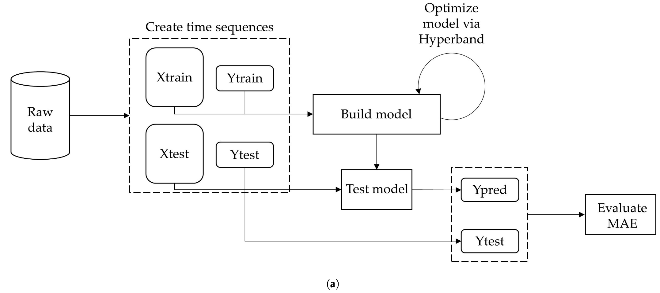
Two types of ML models trained and tested on the multivariable dataset above were the following: (1) supervised models; and (2) semi-supervised models. Both types are designed to detect multiple classes of faults in the same observation. The supervised models capture the system dynamics and detect faults in time sequences. Conversely, the semi-supervised models neglect the system dynamics. Figure 3 shows the flowchart of the FDD workflow for each type of model.

2.5. Supervised Method

The supervised model implemented adopts a Multi-Input Multi-Output (MIMO) approach. In this complex scenario, all variables in a given time window (here, one day) are fed into the model, which outputs their predicted values. This approach aims to spot variable-wise reconstruction errors that could be related to faults. The predicted time sequences can be used to detect anomalies because, if the actual time sequences are compared with the predicted ones, the actual samples that greatly differ from the predicted ones are labeled as anomalies. Reconstruction errors are evaluated through metrics: Mean Absolute Error (MAE), Mean Absolute Percentage Error (MAPE) and Root Mean Square Error (RMSE). The MAE is computed as:

$$\mathrm{MAE}=\frac{1}{\mathcal{T}}\sum _t^{\mathcal{T}}\underset{\mathrm{absolute}\mathrm{error}}{\underbrace{\frac{1}{N}\sum _i^N\left|y_{i,t}-{\widehat{y}}_{i,t}\right|}}.$$

(1)

The MAPE is computed as:

$$\mathrm{MAPE}=\frac{1}{\mathcal{T}}\sum _t^{\mathcal{T}}\frac{1}{N}\sum _i^N\frac{\left|y_{i,t}-{\widehat{y}}_{i,t}\right|}{y_{i,t}}.$$

(2)

The RMSE is computed as:

$$\mathrm{RMSE}=\sqrt{\frac{1}{\mathcal{T}}\sum _t^{\mathcal{T}}\frac{1}{N}\sum _i^N{\left(y_{i,t}-{\widehat{y}}_{i,t}\right)}^2},$$

(3)

where $y_{i,t}$ is the actual sample of features i at time t. ${\widehat{y}}_{i,t}$ is the reconstructed sample of features i at time t. $\mathcal{T}$ is the number of samples. N is the number of features.

Through a time sequence generator, a time window of size l is shifted over the input time series by one time step forward, so that all samples in the window become an input sequence, while the m samples after the window become the corresponding output sequence. All future sequences form the output of the model. In this way, a labeled dataset suitable for supervised methods is obtained.

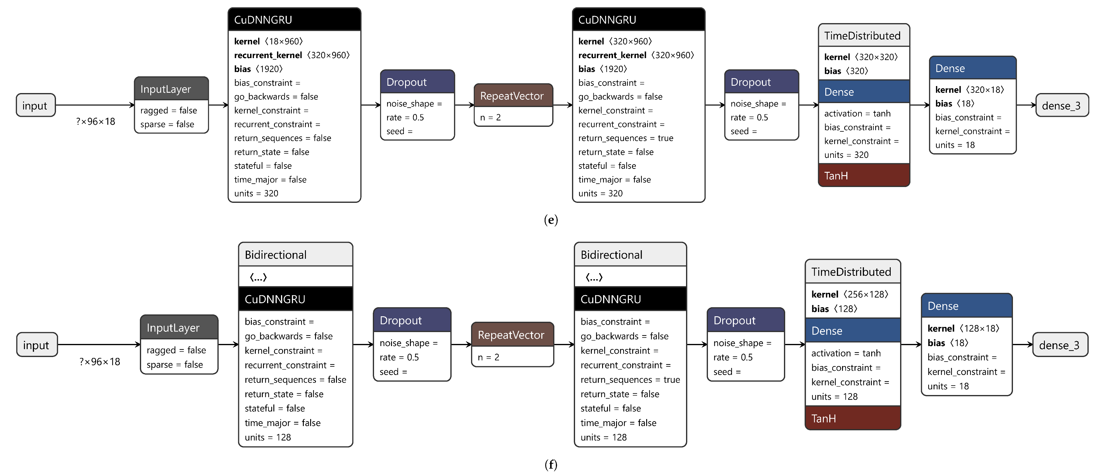
This study stemmed from the poor performance of traditional statistical methods, such as Vector AutoRegression (VAR). Its MAE on the test dataset is equal to 0.23 and too low for FDD in HVAC systems. Therefore, this study analyzed the performance of some RNNs applied to a labeled dataset. Specifically, the hidden layers consisted of Long Short-Term Memory (LSTM) cells and of Gated Recurrent Unit (GRU) cells. LSTMs have hidden states (short-term memory) and cell states (long-term memory), while GRUs only have hidden states.

Variants such as Bidirectional LSTM (BiLSTM) and Bidirectional GRU (BiGRU) were investigated, which add a backward LSTM (GRU) layer to a traditional forward LSTM (GRU) layer. The original input sequence is fed into the forward layer, while the reversed sequence is fed into the backward layer. The outputs of both layers can be combined in several ways, such as concatenation or element-wise sum, average or multiplication. Here concatenation was selected. Bidirectional versions were designed to overcome the shortcomings of traditional versions. They preserve the input information from both past and future at a given time interval, and, hence, long-term relationships are better captured.

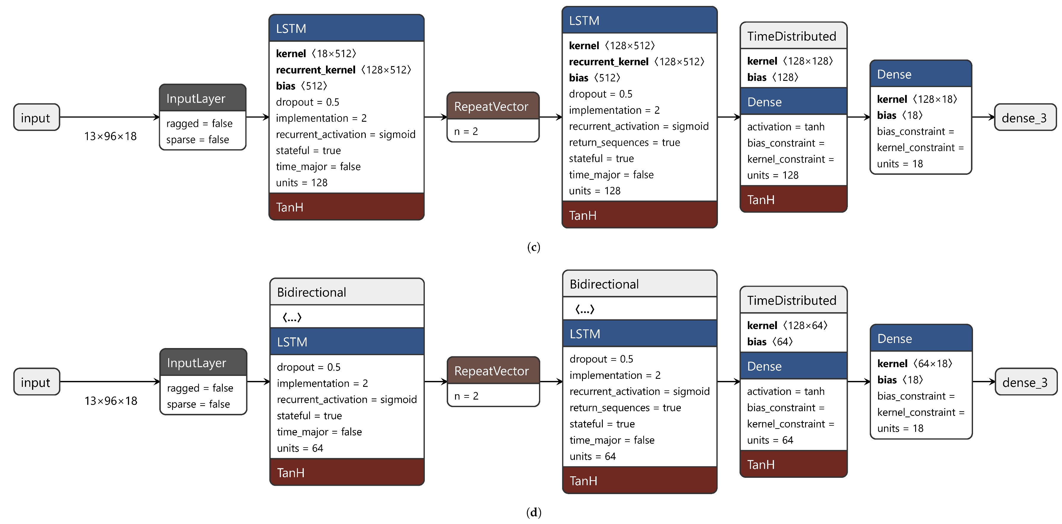
Moreover, the different performance of stateless and stateful networks was examined. Sequence-processing models can be stateless or stateful. Stateless models use sequences of identically distributed and independent training samples, while stateful models consider time dependence between batches. In stateless models, the states of the model are reset each time a new batch is processed. This forces the model to forget the states learned from previous batches. In stateful models, the training batches are assumed to be related to one another. Thus, propagating the learned internal states from one batch to another is useful, as the model better captures the time dependence. As batch size increases, stateless models tend to approach stateful models. Stateful models require batches to be time-sorted, so they can be seen as one sequence, and, hence, shuffling (changing the order of training batches) is not allowed.

This section describes the elements that made up the final network. The network consisted of an input layer, an output layer, and an arbitrary number of intermediate hidden layers. Each layer had a specific activation function. Here, six RNNs were trained and tested. The developed RNNs used the hyperbolic tangent (tanh) as the activation function. This choice enabled the use of the cuDNN implementation, which sped up training [34]. The activation function of the output layer was linear as predicting sequences is a regression problem. The batch size was set to 64 for stateless models and to 13 for stateful models. Stateful models need a batch size that divides the training dataset into equal-size batches. The maximum number of epochs was set to 500. However, to prevent overfitting, an early stopping scheme was set and a dropout of 0.5 was applied to hidden layers as a regularization technique. 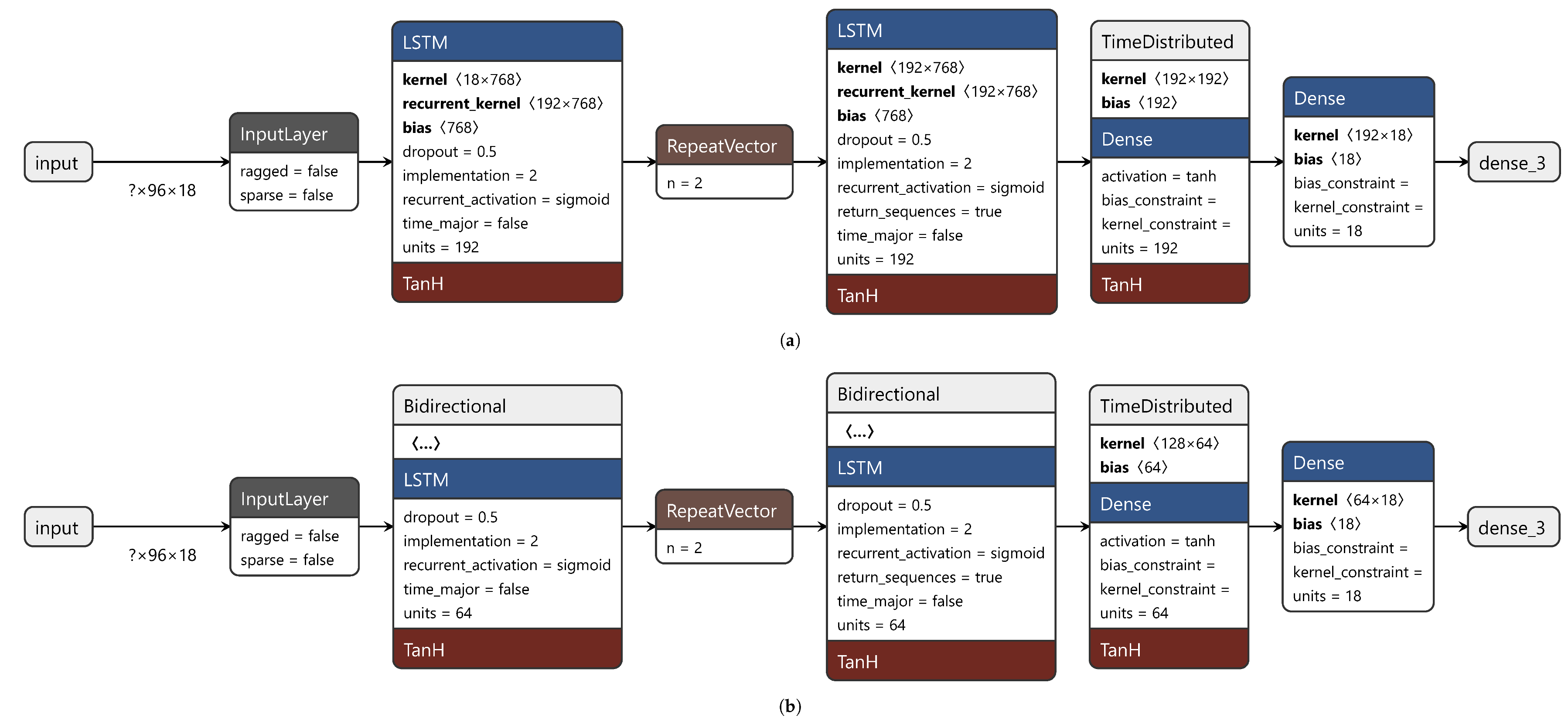The input features are listed in Section 2.3. However, 18 input features were used, because timestamps were replaced by hours and one-hot encoded days of the week. The input size was (96, 18). The sequence length was 96 as the time span considered was 24 h and data was measured and collected every 15 min; hence, 96 measurements spanned a full day’s cycle. The output size was (2, 18). The sequence length was 2 as the model should predict how variables evolve 30 min ahead.

As stated above, this study compared the performance of six variants of a model. This model was an encoder–decoder RNN, which combines the strengths of an autoencoder with those of an RNN. Between two RNN (LSTM or GRU) layers lies a Repeat Vector layer, which allows for a dimensionality reduction of the problem; namely, from 3D to 2D. The RNN layer before the Repeat Vector layer outputs a vector of 2D encoded variables. This vector is decoded by the Repeat Vector layer, which outputs 3D vectors. One of their three dimensions is the number of time steps to be predicted. The network ends with a Time Distributed layer and a Dense layer, which outputs the prediction.

The six variants were:

1.

stateless LSTM;

2.

stateless BiLSTM;

3.

stateful LSTM;

4.

stateful BiLSTM;

5.

stateless GRU;

6.

stateless BiGRU.

Each model was trained and tuned on three hyperparameters: (1) number of hidden layers; (2) number of neurons per hidden layer; (3) L1 and L2 activity regularization in the input layer.

Table 1. Candidate values of the model hyperparameters.

Hyperparameter	Candidate Values
Number of hidden layers	{1, 2, 3}
Number of neurons in the first hidden layer	{$x:x=64n,n\in \{1,\cdots ,6\}$}
L1 and L2 activity regularization factors	{1 × 10 −6, 1 × 10 −5, 1 × 10 −4, 1 × 10 −3}

lists candidate values of these hyperparameters. The Hyperband algorithm of the Keras Tuner [35] automatically tuned the hyperparameters.

The models were trained using Adam as optimizer and using MAE as metrics and as the loss function. The initial dataset was split into training and test datasets, using a 70:30 split ratio. The data split was not random but along time, as the model had to predict the future and keep memory of the past.

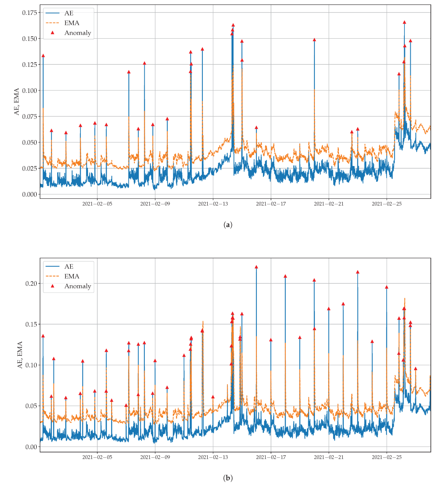
As stated above, the reconstruction errors and performance of the models were evaluated using three metrics: MAE, MAPE and RMSE. Conversely, the anomaly detection was evaluated using the absolute error from Equation (1). This prevented the model from being particularly sensitive to noise, thus, causing false positives. For example, RMSE errors were squared before being averaged, which gave more weight to larger errors. As the data showed seasonal trends, anomalies were detected using a dynamic threshold; namely, using the Exponential Moving Average (EMA) in Equation (4):

$$\begin{array}{cc}\hfill {\mathrm{EMA}}_0& =valu{e}_0,\hfill \\ \hfill {\mathrm{EMA}}_n& =\alpha valu{e}_n+\left(1-\alpha \right){\mathrm{EMA}}_{n-1}\mathrm{if}n>0,\hfill \end{array}$$

(4)

where $valu{e}_n$ is the value of absolute error at time n; ${\mathrm{EMA}}_{n-1}$ is the EMA at time $n-1$; $\alpha$ is a smoothing parameter. Here, $\alpha =\raisebox{1ex}{$10$}\!\left/ \!\raisebox{-1ex}{$22$}\right.$. A higher $\alpha$ gave more weight to the absolute error and made the threshold more sensitive to seasonality. Dynamic thresholds are more sensitive to data behavior than static thresholds.

2.6. Semi-Supervised Method

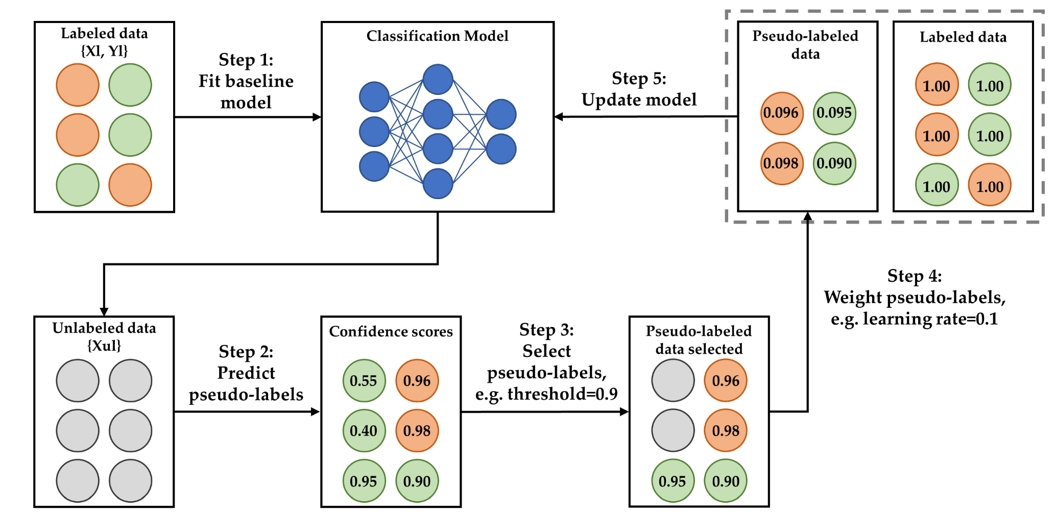
The semi-supervised FDD method implemented built on Fan et al. [23]. There, the self-training strategy was an iterative training process for developing semi-supervised neural networks.

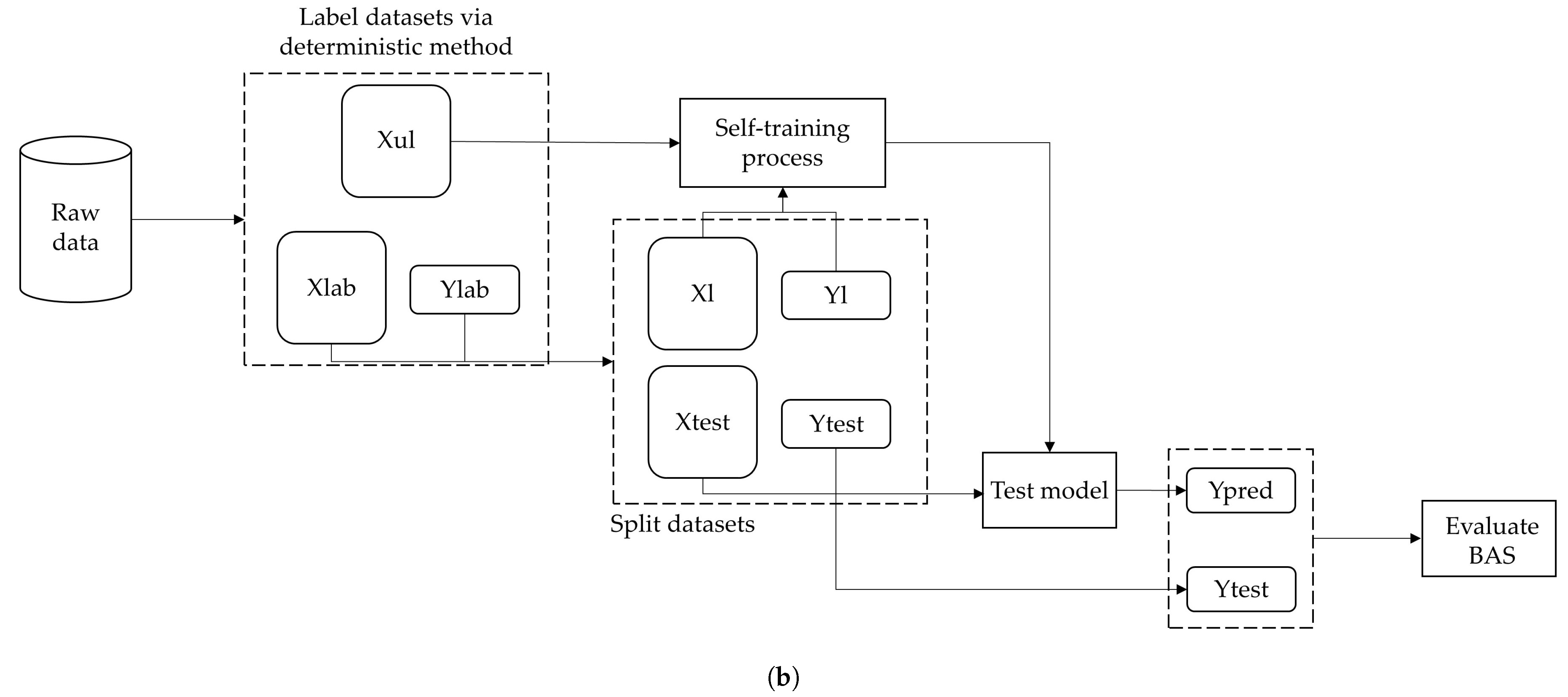
1.

In Step 1, the initial classifier (baseline model) was developed from the small amount of labeled data at hand. Input and output data were termed $X_l$ and $Y_l$, respectively. The train–test split ratio of the labeled dataset for training and testing the classifier at the first learning iteration was set to 20:80. In this way, a consistent test dataset was obtained and its size could be compared with the training dataset, which grew in size during the self-training iterations. The input features are listed in Section 2.3. However, timestamps were replaced by days of the week.

2.

In Step 2. the classifier was tested on the unlabeled data, termed $X_u$, to generate pseudo-labels.

3.

In Step 3, a learning parameter, termed confidence threshold, was introduced to select the pseudo-labels and only pseudo-labels with a relatively high confidence were kept to update the model in the next learning iteration. For example, given a confidence threshold of 0.9, only pseudo-labels with a confidence score of 0.9 or more were kept because they were reliable.

4.

In Step 4, a learning parameter, termed learning rate, which ranged from 0 to 1, was introduced to specify the training weights of the pseudo-labeled data. For example, given a learning rate of 0.1, the weight of a pseudo-labeled data sample with a confidence score of 0.92 was 0.092 (i.e., $0.92\times 0.1=0.092$) in the next learning iteration. Initial data samples were weighted 1.

5.

In Step 5, the whole self-training was rerun to update the classifier.

Figure 4 shows the self-training process.

The self-training strategy was based on three learning parameters: (1) the confidence threshold for the selection of pseudo-labeled data; (2) the learning rate for using the pseudo-labeled data; and (3) the number of learning iterations.

Table 2. Candidate values of the semi-supervised learning parameters.

Parameter	Candidate Values
Confidence threshold	{0.6, 0.7, 0.8, 0.9}
Learning rate	{0.1, 0.2, 0.3, 0.4, 0.5}
Number of iterations	{5}

lists candidate values of these parameters.

As stated in Fan et al. [22], a small confidence threshold enabled the selection of more pseudo-labels for the self-training process and, hence, the model could exploit unlabeled data more efficiently. Conversely, a high confidence threshold removed unreliable pseudo-labels, to strengthen the self-training process.

The self-training strategy assumed a subset of labeled data was available. The labeled data size was 1.16–9.26% of the data size, depending on the labeled data availability per fault [23]. In this study, however, labeled data was missing and, hence, a mix of deterministic methods and clustering was used to label data (i.e., to detect anomalous and normal HVAC data) to start the self-training strategy. The size of the initial labeled dataset thus obtained was equal to 13.8% of the whole dataset, which was deemed enough to label the unlabeled dataset.

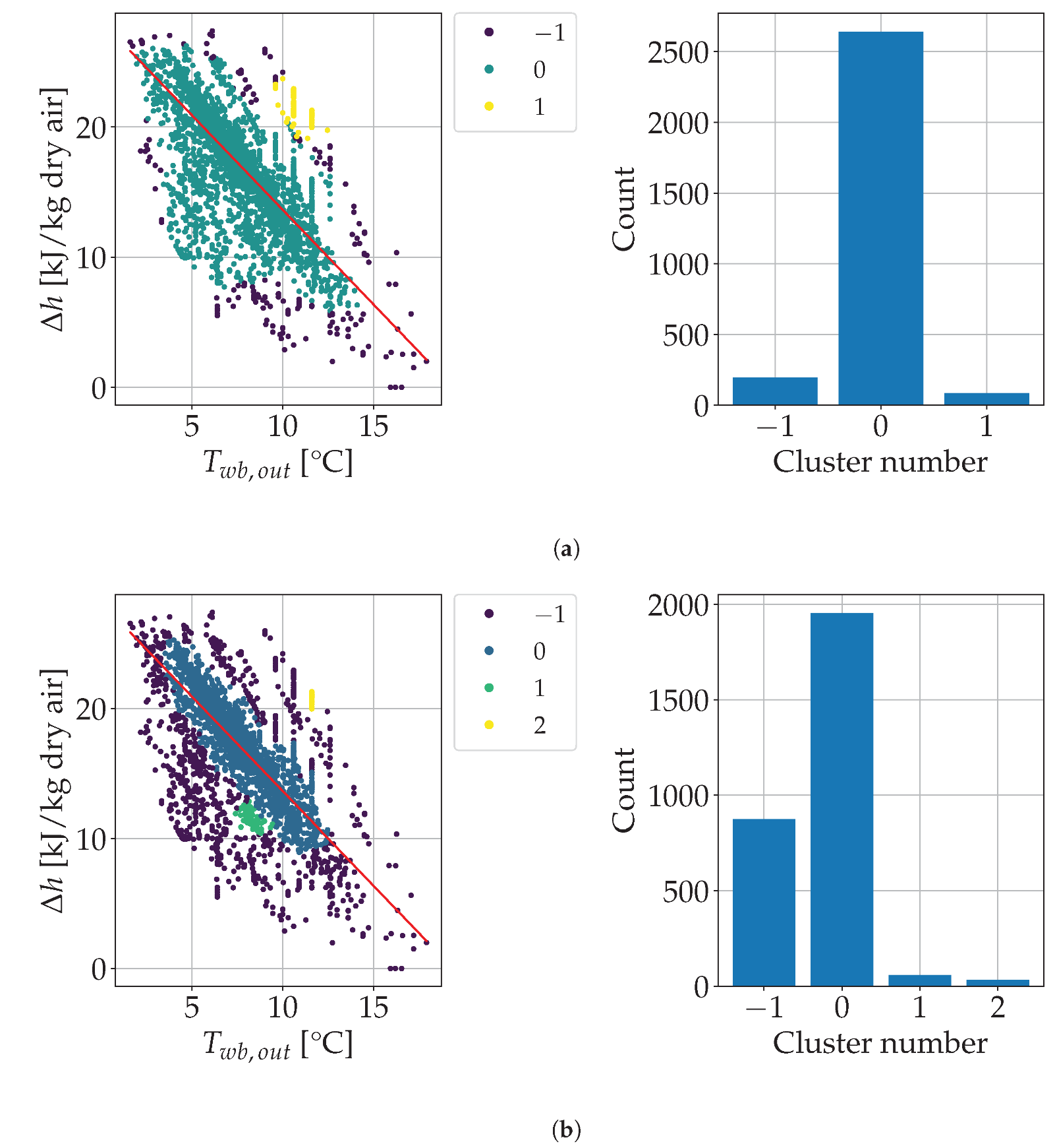
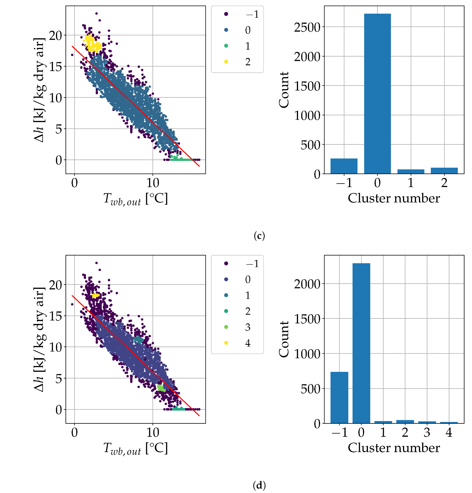
The deterministic methods above should be based on the energy analysis of the HVAC operation. However, the available data and variables did not allow for a comprehensive energy analysis, as many of the variables needed to describe the physics of the problem, such as mass flow rates, valve states (open/closed) and thermal energy usage, were unknown. Deterministic methods help to compute suitable energy Key Performance Indicators (KPIs). These KPIs describe the overall performance and/or operational criteria of an HVAC system. In this work, the main energy KPI was defined as:

$$\mathrm{KPI}(T_{out},R{H}_{out},T_{sup},R{H}_{sup})=\frac{\mathrm{\Delta }h\left(T_{out},R{H}_{out},T_{sup},R{H}_{sup}\right)}{\mathrm{\Delta }\widehat{h}\left(T_{out},R{H}_{out}\right)},$$

(5)

where $T_{out}$ is the dry-bulb temperature of outdoor air; $R{H}_{out}$ is the relative humidity of outdoor air; $T_{sup}$ is the dry-bulb temperature of supply air; $R{H}_{sup}$ is the relative humidity of supply air. Numerator $\mathrm{\Delta }h=h_{sup}-h_{out}$ is the difference between enthalpy of supply air $h_{sup}:h(T_{sup},R{H}_{sup})$ and enthalpy of outdoor air $h_{out}:h(T_{out},R{H}_{out})$. Hence, the numerator gauges the heating provided by the AHU so that air supplied to the room mixes with indoor air and ensures comfort. Denominator $\mathrm{\Delta }\widehat{h}$ is the linear best fit of enthalpy array $\mathrm{\Delta }h$ versus temperature array $T_{wb,out}$; that is,

$$\mathrm{\Delta }\widehat{h}=a{T}_{wb,out}+b,$$

(6)

where a and b are constants determined from Huber regression, a linear regression technique that is robust to outliers. $T_{wb,out}$ is the outdoor wet-bulb temperature, which depends on $T_{out}$ and $R{H}_{out}$. Equation (6) alters the energy signature, that is, the linear best fit of energy demand versus outdoor temperature, to account for outdoor relative humidity, similarly to Krese et al. [36]. Consequently, the KPI in Equation (5) compares the energy required to ensure comfort under current conditions (namely, supply and outdoor conditions) with the energy usually required to ensure comfort under current outdoor conditions.

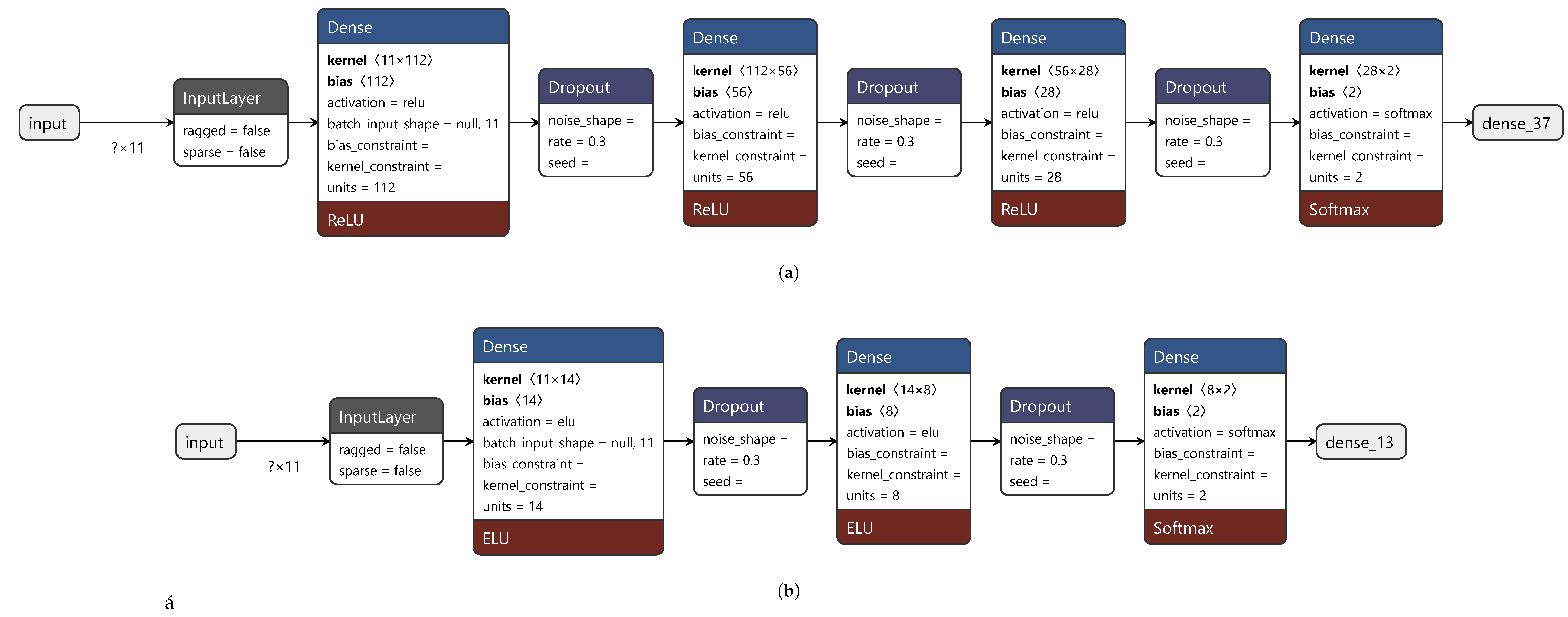
This study stemmed from the poor performance of traditional shallow learning methods, such as Random Forest, whose Balanced Accuracy Score (BAS; see Equation (8)) on the test dataset was equal to 0.65 and too low for FDD in HVAC systems. Therefore, this study analyzed the performance of some ANN classifiers. The self-training aimed to train an ANN classifier. The model should classify data samples as related to faulty or normal operation. The output layer of the model contained two neurons and used softmax as the activation function. Hence, the model output the classification probability; i.e., the likelihood that a data sample belonged to each of the two classes (faulty operation, normal operation). This likelihood was taken as the confidence score. The input layer of the classifier took in all features in the dataset at hand (see Section 2.3) as they were crucial for fault detection. The model was trained using Adam as optimizer, binary cross-entropy as the loss function and accuracy as metrics. The maximum number of epochs was set to 1000. The batch size was set to 64. A dropout of 0.3 was applied to the hidden layers as regularization technique. Moreover, in each learning iteration the model was trained using an early stopping scheme, which stopped the training if the performance of the model on the validation data did not improve after 50 training iterations. Dropout and early stopping prevented overfitting. The model weights from the epoch with the best value of the monitored quantity (here, validation loss) were used in the final model. The validation dataset was the same as the test dataset.

The performance of a classifier depends on the structure of the model and on its hyperparameters. The classifier was trained and tuned on four hyperparameters: (1) activation function; (2) number of hidden layers; (3) number of neurons per hidden layer; (4) L1 and L2 activity regularization in the input layer.

Table 3. Candidate values of the classifier hyperparameters.

Hyperparameter	Candidate Values
Activation function	{tanh, ELU, ReLU, LeakyReLU}
Number of hidden layers	{1, 2, 3}
Number of neurons in the first hidden layer	{$x:x=10+2n,n\in \{0,\cdots ,127\}$}
L1 and L2 activity regularization factors	{1 × 10 −6, 1 × 10 −5, 1 × 10 −4, 1 × 10 −3}

lists candidate values of these hyperparameters.

We designed and tested Algorithm 1 to train the classifier:

Algorithm 1 Function maximized by the differential evolution algorithm. The semi-supervised classifier was trained here.

1: procedureclassifierAccuracy(set of classifier hyperparameters) 2:     use current hyperparameters to update the classifier 3:     for j ∈ sets of learning parameters do 4:         for k ∈ {1, …, number of learning iterations} do 5:            run self-training iteration 6:            compute BAS on the test set 7:         end for 8:         save BAS on the test set as j-th BAS 9:       end for 10:     return best BAS on the test set at current evaluation 11: end procedure

The sets of classifier hyperparameters were combinations of lists in Table 3. The sets of learning parameters were all combinations of lists in Table 2; i.e., their Cartesian product. A differential evolution algorithm [37] as implemented in SciPy 1.8 [38] aimed to maximize the value returned by the procedure in Algorithm 1; i.e., the best BAS on the test set at the last self-training iteration (i.e., at $k=$number of learning iterations), over all sets of learning parameters. To this end, the SciPy algorithm evaluated the procedure up to 180 times, or until relative convergence was met. While doing so, it updated the classifier hyperparameters.

Accuracy Score (AS) and BAS assess the performance of the classifier; i.e., how well it predicts the right class. In binary classification they are defined as:

$$\mathrm{AS}=\frac{TP+TN}{P+N}$$

(7)

and

$$\mathrm{BAS}=\frac{1}{2}\left(\frac{TP}{P}+\frac{TN}{N}\right),$$

(8)

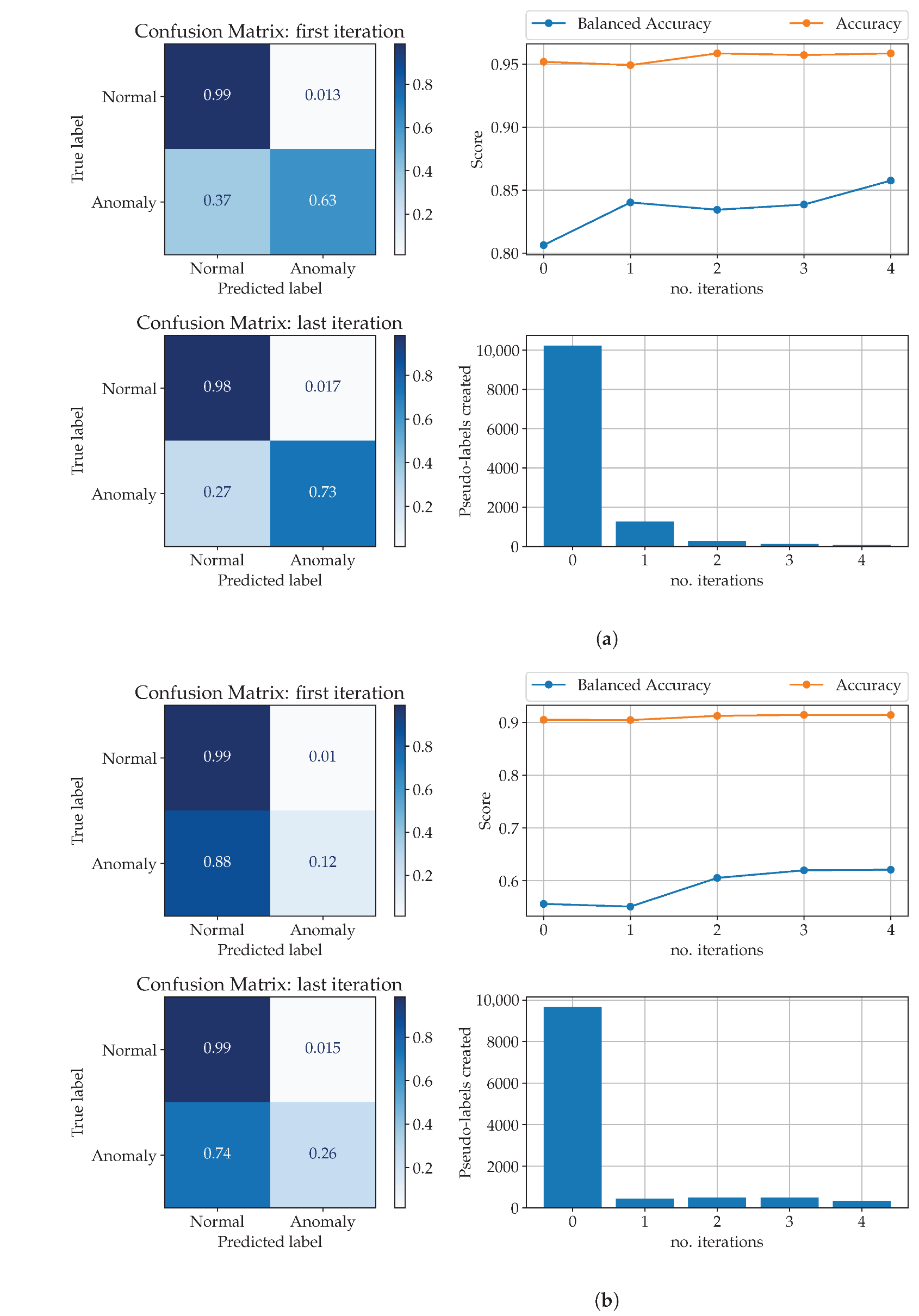
respectively. $TP$ are true positives; $TN$ are true negatives; $FP$ are false positives; $FN$ are false negatives. $P=TP+FN$. $N=TN+FP$. $\raisebox{1ex}{$TP$}\!\left/ \!\raisebox{-1ex}{$P$}\right.$ is termed sensitivity; $\raisebox{1ex}{$TN$}\!\left/ \!\raisebox{-1ex}{$N$}\right.$ is termed specificity. BAS is used for imbalanced datasets. Both BAS and AS range from 0 to 1; the higher the metrics, the better the classification. The classifier was expected to improve its performance during the self-training iterations so that its (balanced) accuracy score at the last iteration was higher than at the first.

All deep learning models used Keras 2.8 [39].

3. Results and Discussion

3.1. Supervised Method

Figure A1 (see Appendix A) shows the final structures of the analyzed networks after hyperparameter tuning. Each structure featured one hidden layer in the encoder and one hidden layer in the decoder. As per Huang et al. [40], an accurate ANN model needs not be large, as oversized networks can lead to large prediction errors. The more complex the model, the more likely it is to overfit the data instead of generalizing its behavior. Hence, the number of neurons in the hidden layers was also low. Dropout and early stopping thwart overfitting.

This analysis aimed to identify the best supervised model for detecting faults. The models were compared in terms of MAE, MAPE and RMSE.

Table 4. Performance metrics results for a 15 min forecast horizon.

Model	MAE	MAPE	RMSE
stateless LSTM	0.075	0.531	0.133
stateless BiLSTM	0.066	0.499	0.110
stateful LSTM	0.122	0.771	0.182
stateful BiLSTM	0.093	0.578	0.160
stateless GRU	0.036	0.242	0.075
stateless BiGRU	0.032	0.230	0.053

and

Table 5. Performance metrics results for a 30 min forecast horizon.

Model	MAE	MAPE	RMSE
stateless LSTM	0.077	0.524	0.141
stateless BiLSTM	0.068	0.494	0.113
stateful LSTM	0.123	0.772	0.184
stateful BiLSTM	0.094	0.579	0.165
stateless GRU	0.042	0.263	0.095
stateless BiGRU	0.034	0.226	0.064

show the performance of the models for a forecast horizon of 15 min and 30 min, respectively.

Table 4 and Table 5 show that the best performing model was the BiGRU. Its MAE was 0.032 for a 15 min forecast horizon and 0.034 for a 30 min forecast horizon. Concerning hyperparameter tuning, the best model featured 5 hidden layers; 256 ($128\times 2$) neurons in the GRU encoder layer; 256 ($128\times 2$) neurons in the GRU decoder layer; 128 neurons in the TimeDistributed layer; 18 neurons in the output Dense layer; and 1 × 10⁻⁶ as L1 and L2 activity regularization factors in the first hidden layer.

Figure 5 shows the anomalies detected by the best model on the test dataset, as explained in Section 2.5. Figure 5a exemplifies anomalies detected for a 15 min forecast horizon. Out of 9698 test samples, 99 were anomalous; that is, 1.02%. Figure 5b exemplifies anomalies detected for a 30 min forecast horizon. Out of 9698 test samples, 184 were anomalous; that is, 1.90%.

The results suggested that, on average, the reconstruction error was small. The best model was able to predict the normal operation of the system with high accuracy; therefore, when the MAE was higher than a certain preset threshold, anomalous operation was detected. The model performed well on the test dataset. Table 4 and Table 5 show that the model performed worse when the forecast horizon was longer. However, the model allowed the timely detection of faults and, hence, the performance over the time horizons examined was considered acceptable. As highlighted in Mtibaa et al. [41] and in Di Già and Papurello [29], the MIMO model appeared to be suitable for predicting the state of the system. Nevertheless, Mtibaa et al. [41] and Di Già and Papurello [29] consider an MIMO model made of LSTM cells. This work highlights how an MIMO network made of GRU encoder–decoders could improve the prediction of the state of the system.

The performance of the stateless BiGRU model was tested on three smaller training datasets, equal to $\raisebox{1ex}{$3$}\!\left/ \!\raisebox{-1ex}{$7$}\right.$, $\raisebox{1ex}{$4$}\!\left/ \!\raisebox{-1ex}{$7$}\right.$ and $\raisebox{1ex}{$5$}\!\left/ \!\raisebox{-1ex}{$7$}\right.$ of the initial training dataset. The test dataset was left unchanged. The MAE on the test dataset increased from 0.032 to 0.073, 0.074 and 0.076, respectively. This result suggested that the performance of the model above improved with a larger training dataset. However, the performance dropped and plateaued out for small training datasets.

3.2. Semi-Supervised Method

Figure 6 shows the modified energy signature in Equation (6). A negative correlation between energy demand and wet-bulb temperature can be noted: the lower the outdoor wet-bulb temperature, the higher the energy demand, and vice versa. However, the analysis conducted was not physically accurate, nor was it meant to be. The KPI in Equation (5) aimed to be a practical tool to tell the normal operation of the HVAC system apart from the anomalous one. Specifically, the farther the points were from the best-fit line (i.e., the farther the KPI in Equation (5) was from 1), the more they marked anomalous operation of the HVAC system.

Unsupervised methods were used to determine the initial labeled dataset (see Section 2.6) from Equation (6). Density-Based Spatial Clustering of Applications with Noise (DBSCAN) was used as the clustering algorithm. DBSCAN used scikit-learn 1.0.2 [42]. Figure 7 shows DBSCAN clusters from two different sets of hyperparameters: Figure 7a,c show the initial subsets of anomalous data for the self-training process in 2019 and 2020, respectively. Likewise, Figure 7b,d show the initial subsets of normal data for the self-training process in 2019 and 2020, respectively. These four subsets formed the initial labeled dataset for the self-training. Two hyperparameters were set here:

1.

$\epsilon$; i.e., the maximum distance between two points for them to be regarded as neighbors.

2.

minPts; i.e., the minimum number of neighbors of a point for it to be regarded as a core point. The point itself is included in minPts.

The selected hyperparameters ensured that the number of anomalous samples was roughly $\raisebox{1ex}{$1$}\!\left/ \!\raisebox{-1ex}{$10$}\right.$ that of normal samples. The initial labeled dataset included 455 anomalies and 4245 normal samples. This outcome matched reality, in that, the number of anomalous samples is usually an order of magnitude lower than that of normal samples. The initial labeled dataset was 28.0% of the whole dataset. Therefore, the dataset was split as follows: 8% of it was the labeled training dataset for training the baseline model; 20% was the labeled test dataset for testing the model; and 72% was the unlabeled dataset.

Concerning semi-supervised learning parameters, confidence threshold$=0.9$ and learning rate$=0.1$ yielded the best balanced accuracy. This was the strictest combination as it allowed pseudo-labeling of data only if the likelihood of belonging to a given class was higher than 90%. Moreover, a small learning rate weighted pseudo-labeled data less to ensure that the model, while self-trained, maintained high performance. As stressed in Fan et al. [23], small learning rates should be used if improving the detection of faults already found in the labeled data is the main goal.

Concerning classifier hyperparameters, Figure A2a (see Appendix A) shows the best model. 3 hidden layers; 112 neurons in hidden layer 1, 56 neurons in hidden layer 2, 28 neurons in hidden layer 3; the Rectified Linear Unit (ReLU) as the activation function in the hidden layers; 1 × 10⁻⁴ as L1 and L2 activity regularization factors in the first hidden layer.

Figure A2b (see Appendix A) shows the worst model: 2 hidden layers; 14 neurons in hidden layer 1, 8 neurons in hidden layer 2; Exponential Linear Unit (ELU) as activation function in the hidden layers; 1 × 10⁻⁴ as L1 and L2 activity regularization factors in the first hidden layer.

Figure 8a shows that the best model was highly accurate throughout the self-training. Moreover, as the self-training proceeded, both accuracy and balanced accuracy score increased, by 1.5% and 5.5%, respectively. The BAS went from 80.5% (first self-learning iteration) to 86% (last self-learning iteration).

Figure 8b shows that the worst model was fairly accurate throughout the self-training. During the self-training both accuracy and balanced accuracy score increased, by 0.5% and 4%, respectively. However, the confusion matrix at the last iteration showed that the model had low classification performance on the test dataset.

As stressed in Albayati et al. [27], the common semi-supervised models can only detect one type of fault at a time, whereas the proposed method enabled the detection of multiple types of faults at once. This matched reality, as many different kinds of faults can occur simultaneously. The good results could allow transfer of knowledge from this AHU to other AHUs, under the same operating conditions.

3.3. Overall Discussion

The results of this HVAC FDD should be interpreted and explained based on the operation of the AHU at hand. Data-driven HVAC FDD should be combined with physical knowledge of the AHU transformations and components (see Section 2.2).

The performance metrics should account for the importance of each feature by, for example, weighting them differently. This is left to future work.

4. Conclusions

The conclusions are summarized below:

• Hyperparameter tuning was performed on six supervised models. Their feature prediction was tested over 15 min and 30 min. The MAE of the best model was 0.032 in the former case and 0.034 in the latter case. The best model could predict both normal and anomalous HVAC operation with high accuracy because its MAE was reasonably low.
• The semi-supervised approach required an initial labeled dataset to label unlabeled samples as normal or anomalous. The percentage of anomalies in the initial labeled dataset closely matched reality, thanks to the deterministic method used and to DBSCAN. Hyperparameter tuning was performed on semi-supervised models. The tuner could test up to 180 models on 20 combinations of learning parameters. The BAS of the best model increased from 80.5% (first iteration of the self-learning process) to 86% (last iteration), which was deemed acceptable to automate HVAC FDD in non-residential buildings.
• The models above do not require extensive feature engineering or fully labeled datasets to perform well and, therefore, they are a stepping stone to transferring data-driven FDD methods from the energy systems of non-residential buildings to other energy systems; e.g., Industry 4.0, smart grids and smart homes.
• These methods are transferable to other energy systems if the amount and quality of historical data are high enough. Similar performance can be expected on AHUs with similar system specifications and monitored variables. However, these models could perform poorly when tackling new operational conditions. MLOps (Machine Learning Operations) pipelines can automatically retrain models if model drift occurs (i.e., lower performance of the model on new data). Future work could focus on transfer learning between similar energy systems with fewer historical samples.

References

1. Hamilton, I.; Kennard, H.; Rapf, O.; Kockat, J.; Zuhaib, S.; Simjanovic, J.; Toth, Z. 2021 Global Status Report for Buildings and Construction: Towards a Zero-emission, Efficient and Resilient Buildings and Construction Sector; United Nations Environment Programme: Nairobi, Kenya, 2021. [Google Scholar]
2. European Commission. Impact Assessment Accompanying the Document “Communication from the Commission to the European Parliament, The Council, The European Economic and Social Committee and the Committee of the Regions Stepping Up Europe’s 2030 Climate Ambition. Investing in a Climate-Neutral Future for the Benefit of Our People”. SWD(2020) 176 Final. Available online: https://eur-lex.europa.eu/legal-content/EN/TXT/?uri=CELEX:52020SC0176 (accessed on 15 January 2023).
3. Thangavelu, S.R.; Myat, A.; Khambadkone, A. Energy optimization methodology of multi-chiller plant in commercial buildings. Energy 2017, 123, 64–76. [Google Scholar] [CrossRef]
4. Rajith, A.; Soki, S.; Hiroshi, M. Real-time optimized HVAC control system on top of an IoT framework. In Proceedings of the 2018 Third International Conference on Fog and Mobile Edge Computing (FMEC), Barcelona, Spain, 23–26 April 2018; IEEE: Barcelona, Spain, 2018; pp. 181–186. [Google Scholar] [CrossRef]
5. Bagheri, A.; Genikomsakis, K.N.; Koutra, S.; Sakellariou, V.; Ioakimidis, C.S. Use of AI Algorithms in Different Building Typologies for Energy Efficiency towards Smart Buildings. Buildings 2021, 11, 613. [Google Scholar] [CrossRef]
6. Yang, H.; Zhang, T.; Li, H.; Woradechjumroen, D.; Liu, X. HVAC Equipment, Unitary: Fault Detection and Diagnosis. In Encyclopedia of Energy Engineering and Technology, 2nd ed.; CRC Press: Boca Raton, FL, USA, 2014. [Google Scholar] [CrossRef]
7. Department of Climate Change, Energy, the Environment and Water of the Australian Government. Factsheet: HVAC Energy Breakdown. Available online: https://www.environment.gov.au/system/files/energy/files/hvac-factsheet-energy-breakdown.pdf (accessed on 15 January 2023).
8. European Commission, Directorate-General for Energy. Proposal for a Directive of the European Parliament and of the Council on the Energy Performance of Buildings (Recast). COM(2021) 802 Final. Available online: https://eur-lex.europa.eu/legal-content/EN/TXT/?uri=celex:52021PC0802 (accessed on 15 January 2023).
9. Kim, W.; Katipamula, S. A review of fault detection and diagnostics methods for building systems. Sci. Technol. Built Environ. 2018, 24, 3–21. [Google Scholar] [CrossRef]
10. American Society of Heating, Refrigerating and Air-Conditioning Engineers. Energy Estimating and Modeling Methods. In ASHRAE Handbook Fundamentals (SI Edition); ASHRAE: Atlanta, GA, USA, 2017; Chapter 19. [Google Scholar]
11. Subramaniam, A.M.; Jain, T. Fault Tolerant Economic Model Predictive Control for Energy Efficiency in a Multi-Zone Building. In Proceedings of the 2018 IEEE Conference on Control Technology and Applications (CCTA), Copenhagen, Denmark, 21–24 August 2018; IEEE: Copenhagen, Denmark, 2018; pp. 205–210. [Google Scholar] [CrossRef]
12. Bianchini, G.; Casini, M.; Pepe, D.; Vicino, A.; Zanvettor, G.G. An integrated model predictive control approach for optimal HVAC and energy storage operation in large-scale buildings. Appl. Energy 2019, 240, 327–340. [Google Scholar] [CrossRef]
13. Mirnaghi, M.S.; Haghighat, F. Fault detection and diagnosis of large-scale HVAC systems in buildings using data-driven methods: A comprehensive review. Energy Build. 2020, 229, 110492. [Google Scholar] [CrossRef]
14. Ebrahimifakhar, A.; Kabirikopaei, A.; Yuill, D. Data-driven fault detection and diagnosis for packaged rooftop units using statistical machine learning classification methods. Energy Build. 2020, 225, 110318. [Google Scholar] [CrossRef]
15. Zhou, Z.; Li, G.; Wang, J.; Chen, H.; Zhong, H.; Cao, Z. A comparison study of basic data-driven fault diagnosis methods for variable refrigerant flow system. Energy Build. 2020, 224, 110232. [Google Scholar] [CrossRef]
16. Masdoua, Y.; Boukhnifer, M.; Adjallah, K.H. Fault Detection and Diagnosis in AHU System with Data Driven Approaches. In Proceedings of the 2022 8th International Conference on Control, Decision and Information Technologies (CoDIT), Istanbul, Turkey, 17–20 May 2022; IEEE: Istanbul, Turkey, 2022; pp. 1375–1380. [Google Scholar] [CrossRef]
17. Taheri, S.; Ahmadi, A.; Mohammadi-Ivatloo, B.; Asadi, S. Fault detection diagnostic for HVAC systems via deep learning algorithms. Energy Build. 2021, 250, 111275. [Google Scholar] [CrossRef]
18. Lee, K.P.; Wu, B.H.; Peng, S.L. Deep-learning-based fault detection and diagnosis of air-handling units. Build. Environ. 2019, 157, 24–33. [Google Scholar] [CrossRef]
19. Shahnazari, H.; Mhaskar, P.; House, J.M.; Salsbury, T.I. Modeling and fault diagnosis design for HVAC systems using recurrent neural networks. Comput. Chem. Eng. 2019, 126, 189–203. [Google Scholar] [CrossRef]
20. Dey, M.; Rana, S.P.; Dudley, S. Semi-Supervised Learning Techniques for Automated Fault Detection and Diagnosis of HVAC Systems. In Proceedings of the 2018 IEEE 30th International Conference on Tools with Artificial Intelligence (ICTAI), Volos, Greece, 5–7 November 2018; IEEE: Volos, Greece, 2018; pp. 872–877. [Google Scholar] [CrossRef]
21. Yan, K.; Zhong, C.; Ji, Z.; Huang, J. Semi-supervised learning for early detection and diagnosis of various air handling unit faults. Energy Build. 2018, 181, 75–83. [Google Scholar] [CrossRef]
22. Fan, C.; Liu, X.; Xue, P.; Wang, J. Statistical characterization of semi-supervised neural networks for fault detection and diagnosis of air handling units. Energy Build. 2021, 234, 110733. [Google Scholar] [CrossRef]
23. Fan, C.; Liu, Y.; Liu, X.; Sun, Y.; Wang, J. A study on semi-supervised learning in enhancing performance of AHU unseen fault detection with limited labeled data. Sustain. Cities Soc. 2021, 70, 102874. [Google Scholar] [CrossRef]
24. Elnour, M.; Meskin, N.; Khan, K.; Jain, R. Application of data-driven attack detection framework for secure operation in smart buildings. Sustain. Cities Soc. 2021, 69, 102816. [Google Scholar] [CrossRef]
25. Li, B.; Cheng, F.; Zhang, X.; Cui, C.; Cai, W. A novel semi-supervised data-driven method for chiller fault diagnosis with unlabeled data. Appl. Energy 2021, 285, 116459. [Google Scholar] [CrossRef]
26. Martinez-Viol, V.; Urbano, E.M.; Torres Rangel, J.E.; Delgado-Prieto, M.; Romeral, L. Semi-Supervised Transfer Learning Methodology for Fault Detection and Diagnosis in Air-Handling Units. Appl. Sci. 2022, 12, 8837. [Google Scholar] [CrossRef]
27. Albayati, M.G.; Faraj, J.; Thompson, A.; Patil, P.; Gorthala, R.; Rajasekaran, S. Semi-Supervised Machine Learning for Fault Detection and Diagnosis of a Rooftop Unit. Big Data Min. Anal. 2023, 6, 170–184. [Google Scholar] [CrossRef]
28. Becchio, C.; Corgnati, S.P.; Crespi, G.; Pinto, M.C.; Viazzo, S. Exploitation of dynamic simulation to investigate the effectiveness of the Smart Readiness Indicator: Application to the Energy Center building of Turin. Sci. Technol. Built Environ. 2021, 27, 1127–1143. [Google Scholar] [CrossRef]
29. Di Già, S.; Papurello, D. Hybrid Models for Indoor Temperature Prediction Using Long Short Term Memory Networks—Case Study Energy Center. Buildings 2022, 12, 933. [Google Scholar] [CrossRef]
30. Standard ISO 7730:2005; Technical Committee ISO/TC 159/SC 5 “Ergonomics of the Physical Environment”. Ergonomics of the Thermal Environment—Analytical Determination and Interpretation of Thermal Comfort Using Calculation of the PMV and PPD Indices and Local Thermal Comfort Criteria. International Organization for Standardization: Geneva, Switzerland, 2005.
31. Standard EN 16798-1:2019; Technical Committee CEN/TC 156 “Ventilation for Buildings”. Energy Performance of Buildings—Ventilation for Buildings. Part 1: Indoor Environmental Input Parameters for Design and Assessment of Energy Performance of Buildings Addressing Indoor Air Quality, Thermal Environment, Lighting and Acoustics. European Committee for Standardization: Brussels, Belgium, 2019.
32. Standard ANSI/ASHRAE 55-2020; ASHRAE Standing Standard Project Committee 55. Thermal Environmental Conditions for Human Occupancy. American Society of Heating, Refrigerating and Air-Conditioning Engineers: Atlanta, GA, USA, 2021.
33. Seyam, S. Types of HVAC Systems. In HVAC System; Kandelousi, M.S., Ed.; IntechOpen: Rijeka, Croatia, 2018; Chapter 4. [Google Scholar] [CrossRef]
34. The TensorFlow Authors. Tf.Teras.Layers.LSTM. Available online: https://www.tensorflow.org/api_docs/python/tf/keras/layers/LSTM (accessed on 15 January 2023).
35. O’Malley, T.; Bursztein, E.; Long, J.; Chollet, F.; Jin, H.; Invernizzi, L.; de Marmiesse, G.; Hahn, A.; Fu, Y.; Mullenbach, J.; et al. Keras Tuner. Available online: https://github.com/keras-team/keras-tuner (accessed on 15 January 2023).
36. Krese, G.; Prek, M.; Butala, V. Analysis of Building Electric Energy Consumption Data Using an Improved Cooling Degree Day Method. Stroj. Vestn. J. Mech. Eng. 2012, 58, 107–114. [Google Scholar] [CrossRef]
37. Storn, R.; Price, K. Differential Evolution—A Simple and Efficient Heuristic for Global Optimization over Continuous Spaces. J. Glob. Optim. 1997, 11, 341–359. [Google Scholar] [CrossRef]
38. Virtanen, P.; Gommers, R.; Oliphant, T.E.; Haberland, M.; Reddy, T.; Cournapeau, D.; Burovski, E.; Peterson, P.; Weckesser, W.; Bright, J.; et al. SciPy 1.0: Fundamental Algorithms for Scientific Computing in Python. Nat. Methods 2020, 17, 261–272. [Google Scholar] [CrossRef] [PubMed]
39. Chollet, F.; Rahman, F.; Pumperla, M.; Santana, E.; McColgan, T.; Snelgrove, X.; Oliver, M.; Matsuyama, M.; Schmidt, P.; Santos, J.F.; et al. Keras. Available online: https://keras.io (accessed on 15 January 2023).
40. Huang, H.; Chen, L.; Hu, E. A neural network-based multi-zone modelling approach for predictive control system design in commercial buildings. Energy Build. 2015, 97, 86–97. [Google Scholar] [CrossRef]
41. Mtibaa, F.; Nguyen, K.K.; Azam, M.; Papachristou, A.; Venne, J.S.; Cheriet, M. LSTM-based indoor air temperature prediction framework for HVAC systems in smart buildings. Neural Comput. Appl. 2020, 32, 17569–17585. [Google Scholar] [CrossRef]
42. Pedregosa, F.; Varoquaux, G.; Gramfort, A.; Michel, V.; Thirion, B.; Grisel, O.; Blondel, M.; Prettenhofer, P.; Weiss, R.; Dubourg, V.; et al. Scikit-learn: Machine Learning in Python. J. Mach. Learn. Res. 2011, 12, 2825–2830. [Google Scholar]
Figure 1. The Energy Center.
Processes 11 00535 g001
Figure 2. Front section of the AHU. Numbers mark sensors and meters: 1: Outdoor temperature and humidity. 2: Supply air temperature and humidity. 3: Return air temperature and humidity; temperature setpoint. 4: Saturation temperature. 5: Power and energy of plug fans.
Processes 11 00535 g002
Figure 3. FDD workflow developed for each type of model. (a) Flowchart of supervised models. (b) Flowchart of semi-supervised models.
Processes 11 00535 g003aProcesses 11 00535 g003b
Figure 4. Self-training process. Dashed region refers to new labeled training dataset.
Processes 11 00535 g004
Figure 5. Anomalies detected. An anomaly occurs when the absolute error (AE) exceeds the EMA. A subset of the anomalies detected on the test dataset is shown for clarity. (a) Anomalies detected for a 15 min forecast horizon. (b) Anomalies detected for a 30 min forecast horizon.
Processes 11 00535 g005
Figure 6. Left: Kernel Density Estimation (KDE) plots. KDE estimates the probability density of the samples in the dataset. Red line: energy signature from Equation (6). Right: T w b , o u t (top) and Δ h (bottom) in each winter. (a) Winter 2019–2020. (b) Winter 2020–2021.
Processes 11 00535 g006
Figure 7. DBSCAN clusters used as initial labeled data (anomalies, normal data) in the self-training process. Red line: energy signature. (a) Winter 2019–2020. 3 clusters. ε = 1.1 . minPts = 30. Points in cluster −1 are anomalies. (b) Winter 2019–2020. 4 clusters. ε = 0.7 . minPts = 30. Points in cluster 0 are normal data. (c) Winter 2020–2021. 4 clusters. ε = 0.5 . minPts = 20. Points in cluster −1 are anomalies. (d) Winter 2020–2021. 6 clusters. ε = 0.4 . minPts = 20. Points in cluster 0 are normal data.
Processes 11 00535 g007aProcesses 11 00535 g007b
Figure 8. Performance of best and worst classifier. Confidence threshold = 0.9 . Learning rate = 0.1 . (a) Performance of the best model. (b) Performance of the worst model.
Processes 11 00535 g008