Abstract
We modified the Zwart–Gerber–Belamri (ZGB) cavitation and RNG turbulence models based on their rotational motion characteristics, as well as simulating the phenomenon of small fluctuations in rotational speed due to the action of hydraulic excitation force, to increase the precision of numerical simulations of the cavitation characteristics of centrifugal pumps. According to the theory behind the enhanced model, the pressure gradient in the impeller runner changes uniformly, and the cavitation bubble initially manifests itself at the front edge of the blade’s suction. With the reduction in the effective margin, changes in the impeller flow channel’s pressure gradient increased, the blade’s suction-side cavitation area expanded, and the flow field’s internal disturbance enhanced, resulting in hydraulic loss to the centrifugal pump, considerably reduced operating performance, and the blade pressure side by the cavitation-affected area becoming smaller. The blade’s suction-surface pressure–load curve can be divided into a low-pressure cavitation zone, a pressure fluctuation zone, and a pressure stabilization zone. The pressure–frequency-domain diagram of each monitoring point has a discrete distribution, and the main frequency is the blade-passing frequency ƒ = 293 Hz and its n times frequency. With the deepening of the cavitation, the amplitude of the main frequency in the low-frequency band showed a trend of increasing and then decreasing, and the amplitude of the high-frequency band showed an increasing trend. When we applied the ZGB cavitation model based on the improved rotational motion characteristics to our numerical calculation of the centrifugal pumps’ cavitation characteristics, our calculated cavitation performance curve was closer to the experimental value than the ZGB model, and when the centrifugal pump’s cavitation degree was increased, the area covered by the vacuole area was 1/4 of the suction side of the vane.
1. Introduction
Centrifugal pumps are widely used in various fields because of their simple structure, low cost, and stable performance as highly versatile rotating machines. From water for daily life to daily industrial production, and from agricultural irrigation to large water conservation projects, which are the lifeblood of the national economy, centrifugal pumps play an irreplaceable role.
Centrifugal pumps affect internal flow-field movement due to the roles played by blade rotation and bending, so that the internal flow field is mostly rotational shear turbulence, characterized by dynamic–static coupling, mainstream and boundary layers, flow separation, a reverse-pressure gradient, turning flow, and a variety of more complex hydrodynamic phenomena [1].
Cavitation has an adverse effect on centrifugal pumps and constitutes one of their most common failures: the cavitation phenomenon generated by the bubble reduces the centrifugal pump head’s operating efficiency, as well as negatively affecting other performance parameters; furthermore, these bubbles damage the overflow components, reducing the centrifugal pump’s lifespan. Because the cavitation process is accompanied by vibration noise phenomena, it will also have an impact on some hidden defense equipment [2,3]. There are also constraints on the miniaturization of centrifugal pumps due to cavitation failures. Cavitation cannot be completely avoided [4] in centrifugal pumps’ operation, and engineering applications are generally used to minimize the probability of cavitation failure in centrifugal pumps through structural optimization and improving operating conditions, such as improving the structure of overflow components and increasing the pressure at the centrifugal pump inlet. To maintain centrifugal pump equipment in normal operation, the centrifugal pump’s cavitation status needs to be monitored in real time, so that cavitation failures can be prevented. Therefore, identifying the cavitation status of centrifugal pumps is of considerable research value, providing technical reference for the identification of other types of centrifugal pump failures.
Cavitation is a complex hydrodynamic phenomenon. When the fluid basin’s low-pressure region is below the liquid’s saturation vapor pressure at the corresponding temperature, the liquid vaporizes to produce a vacuolated region and expands continuously, and when the vacuole extends to the high-pressure region, the vacuolated region contracts and eventually collapses. The process from the creation to the collapse of the vacuole is called cavitation [5,6].
Numerical simulation studies for the entire fluid domain inside a centrifugal pump are developing quickly alongside the maturation of CFD fluid dynamics computational theory technology. Desheng Zhang et al. [7] modified the Rayleigh–Plesset cavitation model’s pressure and viscosity coefficients to ensure that the numerical simulation was similar to the experimental values of the centrifugal pump’s inner stream field under high-flow conditions. Tseng and Wang [8] found that the generality of the empirical coefficients can be improved by selecting the appropriate evaporation condensation coefficients in the turbulent flow model. To rectify the empirical coefficients of three separate cavitation models, Morgut [9] aggregated experimental data. Liu et al. [10] concluded that both evaporation and condensation factors in the ZGB cavitation model had significant effects on the predicted centrifugal pump head curve. Evangelos Stavropoulos-Vasilakis et al. [11] published a complete presentation of numerical methods for cavitation modeling, highlighting the connections between applications and methods.
The purpose of this paper is to study the cavitation failure mechanism of a test pump, using the fluid analysis software Fluent to numerically simulate the flow field inside the test pump cavitation, and to improve the original ZGB cavitation model and RNG k-ε turbulence model on the basis of previous theories; a numerical calculation method is proposed to improve the ZGB cavitation model based on the rotational motion characteristics, considering that within the impeller runner rotating at high speed, with a certain size of At the same time, the small fluctuation in rotational speed caused by the action of hydraulic excitation force can be simulated. Then, with the help of this theoretical model, the development process and internal flow-field characteristics of the cavitation state of the test pump are investigated to provide theoretical guidance for the original vibration signal acquisition.
This paper mainly uses Fluent numerical simulation to study the cavitation characteristics of the centrifugal pump. O. Supponen et al. [12] observed cavitation bubble production under high pressure via high-speed imaging. M. Ghorbani [13] et al. presented the visualization and image processing of spray structures affected by cavitation bubbles and cavitation flow patterns. If the conditions allow, the visualization test can be introduced and combined with the simulation results for observation and comparison, which can more intuitively show the development process of the centrifugal pump’s cavitation state and internal flow-field characteristics. In turn, the theoretical model can be used to explore the cavitation failure mechanism of the centrifugal pump and provide theoretical guidance for the design of the signal acquisition scheme.
2. Computational Model and Meshing
The cantilever centrifugal pump model adopted for our study was the IS-65-50-160 single-stage, single-suction pump with number of blades Z = 6 and specific speed ns = 81.5. The basic performance parameters were as follows: flow rate Q = 50 m3/h, head H = 34 m, and speed ne = 2930 r/min. We performed a three-dimensional hydraulic modeling of the test pump’s components using Unigraphics NX, which contains four calculation domains, namely, the inlet section, impeller, worm gear housing, and outlet section (Figure 1).
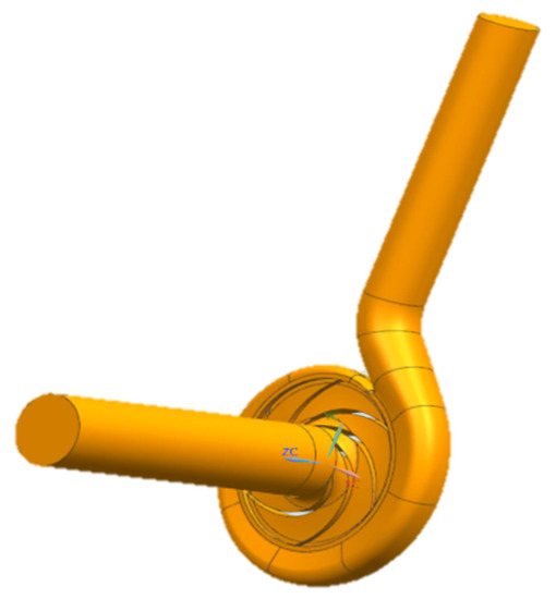
Figure 1.
Three-dimensional model of the computational domain.
We performed a structured hexahedral meshing of the model pump’s four calculation fields using ICEM software. To improve the numerical simulation’s reliability, it is also essential to confirm the grid independence. The higher the number of grids, the smaller the amount of numerical calculation errors due to the number of grids [14]; however, too many grids will also consume a lot of computational resources. Therefore, we utilized four sets of structured grids with different grid numbers for single-phase constant-flow calculation, and we used the centrifugal pump head’s variation under design conditions to determine the suitable grid numbers. Table 1 shows that when the number of grids goes beyond 291,000, the head ceases to alter. Therefore, we chose the third grid solution, as illustrated in Figure 2.

Table 1.
Grid-independent verification.
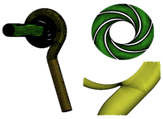
Figure 2.
Model pump and meshing of each computational domain.
3. Numerical Computation Theoretical Model
3.1. Selection and Correction of the Turbulence Model
At present, the numerical simulation of turbulence can be summarized into three methods [15]: direct numerical simulation, large-eddy simulation, and Reynolds time-averaged methods. The centrifugal pump’s operation in the internal flow field constantly undergoes irregular flow changes, meaning that the internal flow fields of the worm and impeller result in different vortex shapes and sizes. The larger vortices are related to the working parameters and geometric structure, which can be used as the vortex structure when characterizing the flow field, which is distributed according to certain rules and exists for a long time. At the same time, there are also many smaller vortices in the flow-field area, which are characteristic of randomly disordered distribution. Due to the large variation in each time and space characteristic scale in the turbulent flow inside the centrifugal pump, it is difficult to directly solve the actual flow problem using the momentum equation. To solve this problem, the momentum equation is usually averaged on the time characteristic scale to focus on the flow-field characteristics on the average time scale inside the centrifugal pump, and the momentum equation processed by the average time characteristic is called a Reynolds time-averaged equation. The Reynolds time-averaged method is widely adopted and used in engineering calculations because of the model’s low requirements regarding the grid’s quality and parameter settings. Two main turbulence models are established by the Reynolds time-averaged equation; however, we made use of the RNG k-ε model [16]. In the event of strong cyclonic flow, the RNG k-ε model has a higher computational precision and takes the turbulent vortices into consideration. The expressions for the turbulent kinetic energy k and the turbulent dissipation rate ε in the constrained equation for the incompressible flow of a constant flow are as follows:
The values of the constants in the above equations are = 0.0845, = 0.012, = 1.42, = 1.68, = 1.0, and = 1.3.
For the centrifugal pump impeller’s geometric modeling and cavitation gas–liquid two-phase flow characteristics, we added the curvature and density correction constraint equations to the RNG k-ε model [17].
The curvature correction is the addition of a curvature correction coefficient to the turbulent kinetic energy generation term Gk, with the expression of the coefficient as follows:
where the values taken for the constant terms are = 1.0, = 2.0, and = 1.0, while r is the mixed homogeneous volume fraction. The RNG k-ε model’s density adjustment modifies the turbulent viscosity, and the correction formula is as follows:
where is the gas-phase density (kg/m3), is the mixed homogeneous-phase density (kg/m3), is the liquid-phase density (kg/m3), and the constant takes the value of 10.
3.2. Selection and Correction of the Cavitation Model
We calculated the overall interphase mass transfer rate per unit volume using the vacuole number density and mass change rate in the ZGB cavitation model. The individual vacuole mass transfer rates are as follows:
The evaporative phase mass transfer rate is expressed as:
The expression for the condensed-phase mass transfer rate is as follows:
where is the nucleation volume fraction, taken as 4 × 10⁻⁴; is the evaporation coefficient, taken as 50; is the condensation coefficient, taken as 1 × 10⁻³; and RB is the bubble radius, taken as 2 × 10⁻⁶.
The conventional ZGB cavitation model, in which RB is an empirical constant, does not consider the effects of the rotational characteristics inside the centrifugal pump on the vacuole morphology. Minemura and Murakami’s study found [18,19] that when the vacuole flows along the edge of the vane, turbulence and shear forces rupture the vacuole into many small bubbles above a specific diameter, which implies the existence of a maximum bubble size in the pump. Here, we improved the ZGB cavitation model based on the previous study.
Through practical and theoretical research, Wan determined the maximum vacuole radius in the centrifugal pump based on the velocity n and the number of blades z [20]:
The average size of bubbles in the cavitation cloud diagram is about 0.6 times the maximum size Rm, and the maximum size of bubbles Rm is inversely proportional to the square root of the turbulent kinetic energy k. Because of the computation’s stability, RB can therefore be reformulated as a function of speed n and blade count z as follows:
By substituting the redefined RB expression into the original ZGB cavitation model, the improved cavitation model can be expressed as follows:
The evaporative-phase mass transfer rate is expressed as
The expression for the condensed-phase mass transfer rate is
where is the evaporation coefficient, taken as 5000; and is the condensation coefficient, taken as 1 × 10⁻³.
When using Fluent to calculate a centrifugal pump’s cavitation inside its flow field, the rotational speed n is fixed by design. However, our experiment found that the rotational speed n was not constant. Hui Sun [21] utilized Fluent and MATLAB to simulate an electric motor and a model centrifugal pump to examine how the motor’s electromagnetic torque affected the centrifugal pump’s speed. Yihang Guo [22] explained how the rotor shaft system affected the centrifugal pump’s rotor velocity, which was affected by the combined action of water, the machine, and electricity and was not a fixed value.
In our study, if the motor output shaft power P and motor rotational inertia were constant, and considering only the effect of the variation in the hydraulic torque of the centrifugal pump on the impeller speed, the speed could be modified as follows:
where is the time step, n’ is the rotational speed in the previous time step, m is the output hydraulic torque in the previous time step, P is the output shaft power, and is the motor rotational inertia, taken as 0.0449 kg·m2.
Using Fluent’s UDF function, we input the transient hydraulic moment m at each step of the centrifugal pump’s non-constant flow calculation output into the mount function by writing the definition EXECUTE_AT_END macro, while the estimated rotational speed served as the starting point for our calculation of the following time-step iteration. Figure 3 shows the running flow.
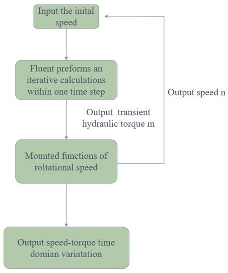
Figure 3.
Flowchart of Fluent UDF macro-operation.
3.3. Boundary Conditions and UDF Settings
We used the modified RNG k-ε turbulence and ZGB cavitation models to numerically simulate the centrifugal pump’s cavitation flow field. First, we performed single-phase steady-state calculations for the centrifugal pump to improve the convergence speed; then, we activated the mixed multiphase flow and cavitation models to perform a steady-state calculation of the two-phase flow in the cavitation state. We used the calculation results of the steady-state flow in the cavitation state as the initial values for our unsteady-state calculation. We set the ambient temperature and atmospheric pressure to 25 ℃ and 0, respectively. We set the flow medium to water vapor and water with a saturated vapor pressure of 3540 Pa. Table 2 shows the boundary conditions in the entire computational fluid domain; the inlet is the total pressure inlet, the outlet is the mass flow outlet, the volume fraction of the liquid phase at the inlet and outlet boundaries is set to 1, and the volume fraction of the vapor phase is set to 0.
Table 2.
Boundary condition setting of the computational domain.
We chose the coupled pressure algorithm as our solution method, and we also chose the least-squares cell-based and PRESTO! pressure discretization formats. Furthermore, we controlled the centrifugal pump’s cavitation severity by varying the total inlet pressure. For the steady-state calculation, we monitored the head to characterize whether the calculation was converged or not, and we considered the steady-state calculation as converged when the head H tended to be stable. For our unsteady-state calculation, we set the time step to ts = T/360 = 5.6883 × 10⁻⁵ s, where T is the rotation period, i.e., each 1° of impeller rotation is a time step, while we set the calculation iteration residual to 10−4, and the total calculation time was 3600 time steps, while convergence was achieved in about 80 steps.
The UDF function can be used to modify or control the computational model or flow during Fluent computation. The program we wrote runs as a compiled function, which is imported, compiled, and embedded in a shared library to communicate with Fluent.
4. Analysis of Calculation Results
4.1. Cavitation Performance Results
We varied the inlet pressure to control the cavitation severity in the internal flow field at a fixed outlet flow rate. The centrifugal pumps’ effective cavitation margin NPSHa is expressed as follows:
where is the total inlet pressure (Pa), is the saturated vapor pressure (Pa), is the inlet flow rate (m/s), ρ is the liquid-phase density (kg/m3), and g is the acceleration of gravity (m/s2).
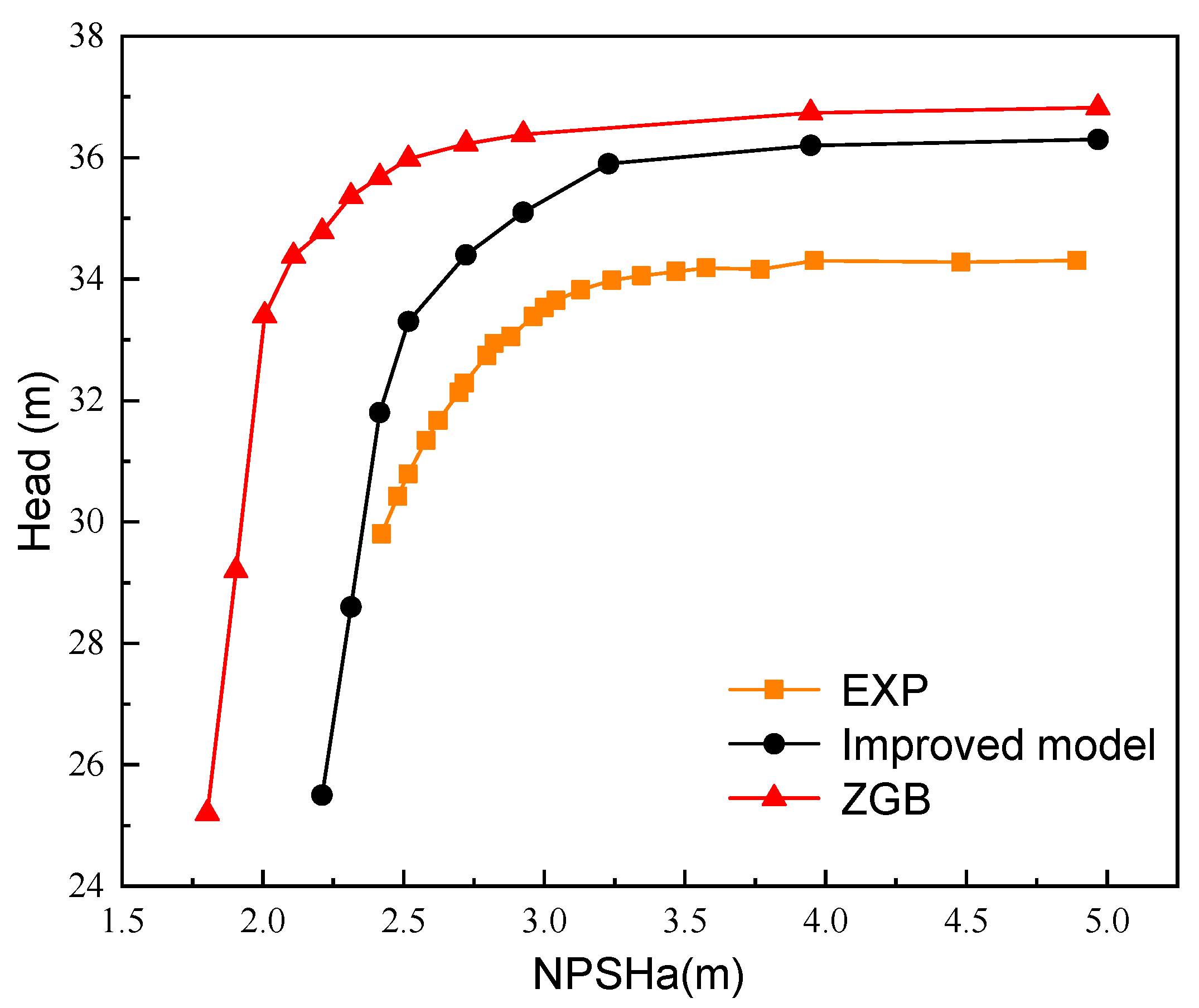
Figure 4 compares our experimental results with the cavitation performance curves before and after improvements to the cavitation and turbulence models.
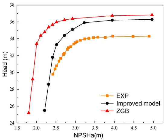
Figure 4.
Comparison of cavitation performance curves.
When the effective cavitation margin was large, the head of the pump was relatively stable; however, as the effective cavitation margin decreased to a certain point, the pump’s head started to drop, and cavitation started to emerge. The centrifugal pump’s head considerably decreased as the effective cavitation margin shrank, causing serious pump cavitation. The critical cavitation margin is the effective cavitation margin when the centrifugal pump head decreases by 3%, and the test pump’s critical cavitation margin was 2.95 m, which was 2.41 m and 2.93 m before and after improvements to the model, respectively, and the improved cavitation performance curve was more similar to the test statistic. Table 3 shows the unsteady-state calculation carried out at four selected operating points.
Table 3.
Calculated working points.
4.2. UDF Speed Output under Cavitation Conditions
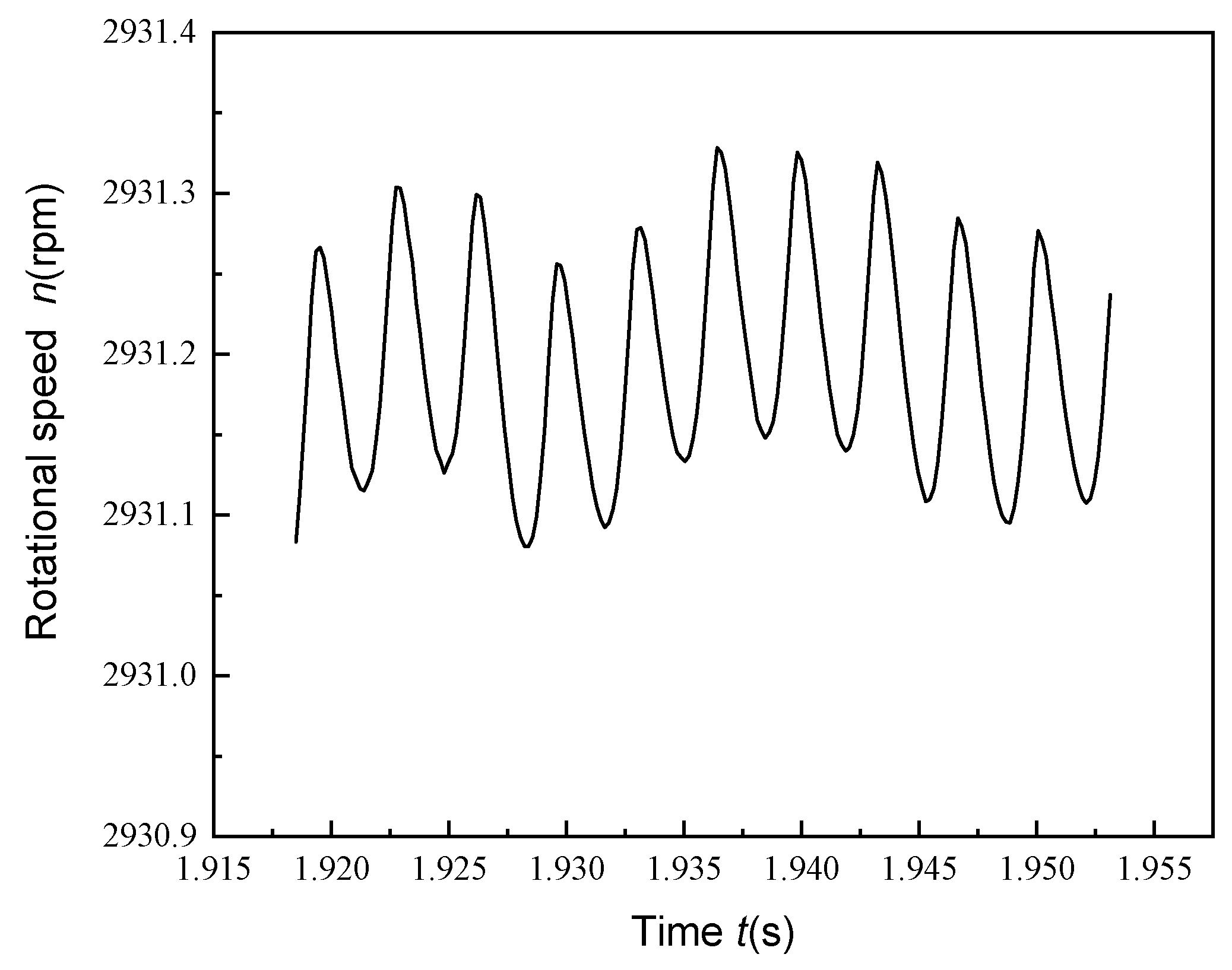
One of the crucial operating factors for centrifugal pumps is rotational speed. Additionally, this is associated with centrifugal pumps’ variations in internal hydraulic torque, which result in small fluctuations in pump speed. In our study, we performed speed correction using the UDF mount function, and the resulting speed fluctuation waveforms were relatively similar in all four operating conditions. As an example, Figure 5 shows the time-domain diagram of the speed fluctuation from the UDF output after the non-stationary numerical calculation stabilization under the cavitation priming condition, and the waveform shows a triangle with obvious periodicity and very small fluctuations near the rated speed.
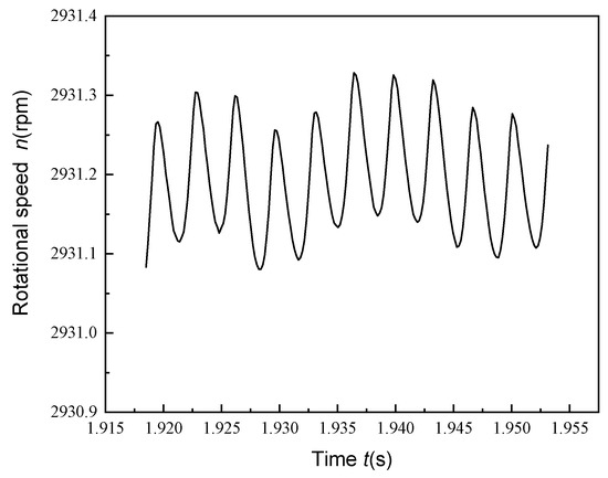
Figure 5.
Time-domain diagram of the centrifugal pump’s speed fluctuations.
4.3. Impeller Runner Static Pressure Field Analysis
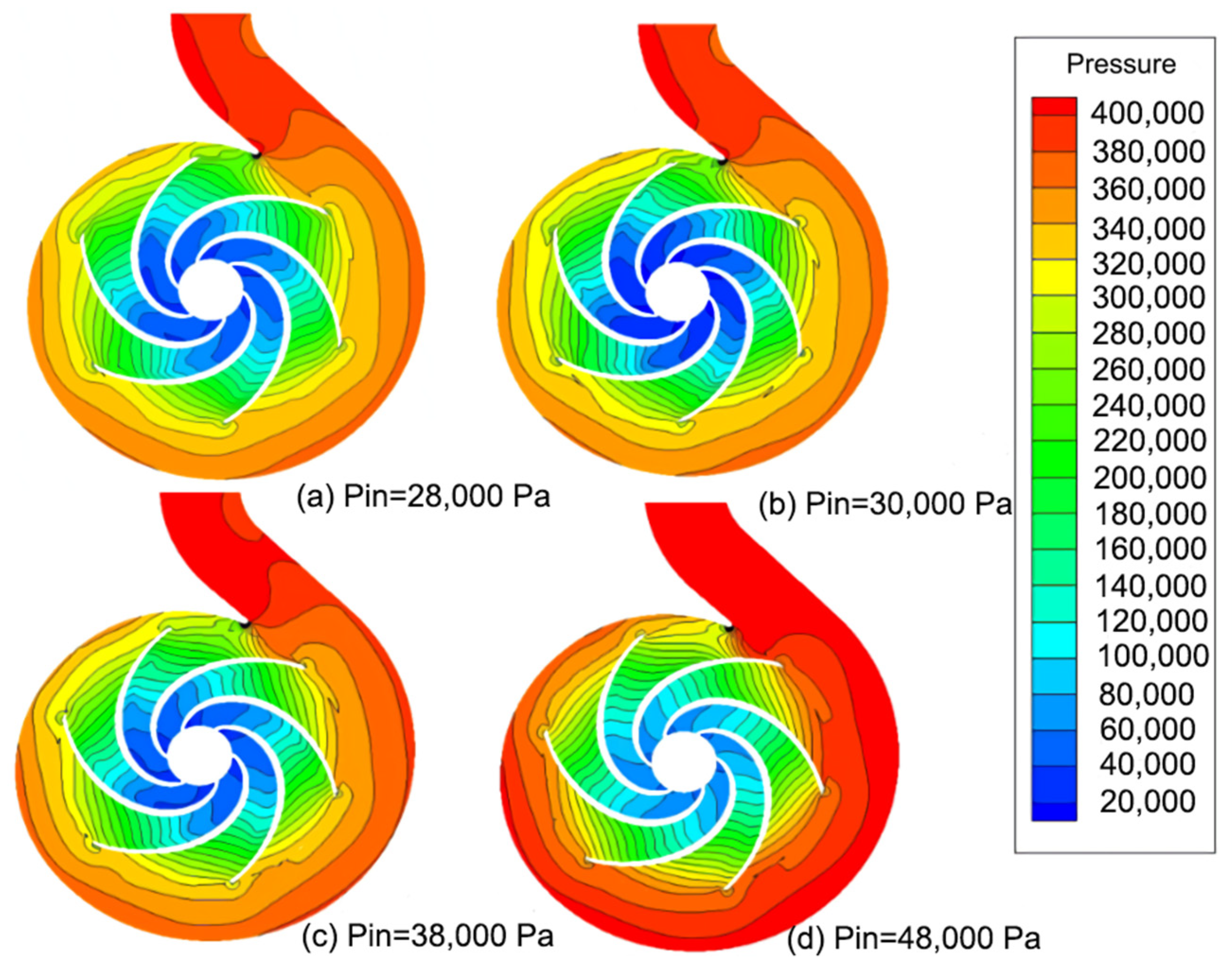
Figure 6a–c show that when the effective cavitation margin is reduced, the blade’s low-pressure suction-surface region begins to increase. When the cavitation phenomenon is more serious, the blade’s low-pressure suction-surface area begins to expand to the front edge of the blade. Figure 6a,b show that, when the effective cavitation margin is lower than the critical cavitation margin, the suction side of the vane’s flow channel is an almost entirely low-pressure area, affecting the pump’s operating performance.

Figure 6.
Static pressure distribution of centrifugal pumps at different NPSHs.
4.4. Analysis of Relative Velocity Distribution of the Impeller Runners
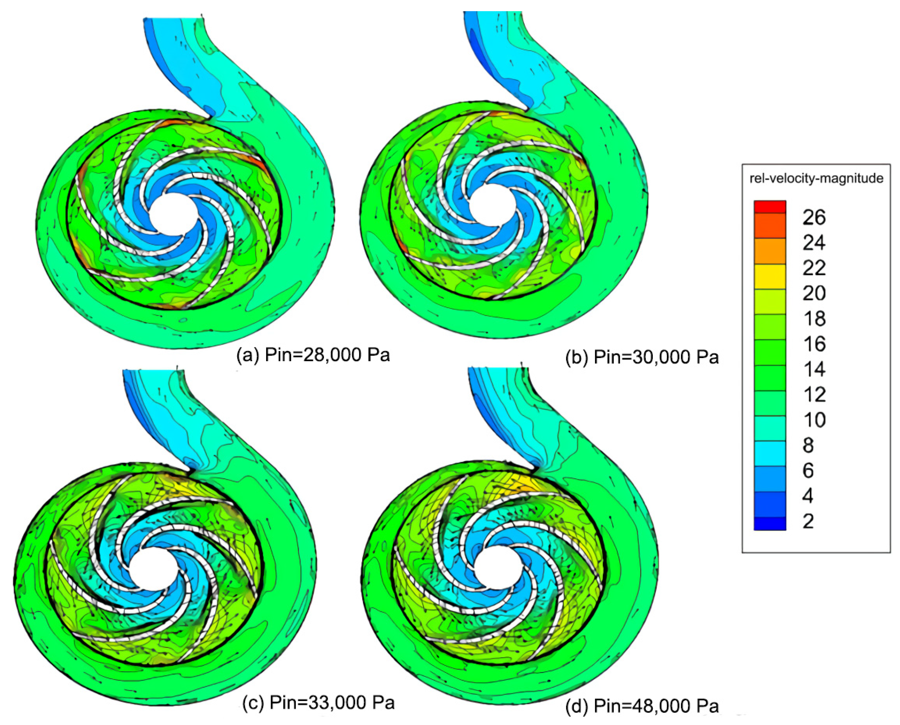
Figure 7 shows the cloud plot of the centrifugal pump’s relative velocity distribution under different effective cavitation margins. Figure 7 illustrates how the impeller flow channel’s relative velocity profile is close to the velocity profile in the steady-state flow field in the non-cavitating condition when the effective cavitation margin is higher than the critical cavitation margin. The cavitation phenomenon only exists in the leading edge of the blade’s suction position, and the impact on the internal flow field is very small. The relative velocity distribution progressively increases along the middle runner of the impeller, and there is a local high-speed area at the posterior edge of the vane’s surface pressure. At the leading edge of the vane’s surface pressure, there is a local low-speed area. Figure 7 shows that when the effective cavitation margin is lower than the critical cavitation margin, the local low-speed area on the pressure side of the blade starts to expand to the impeller runner, causing the blockage of the runner, and there is an obvious local high-speed area at the trailing edge of the blade’s suction side, which keeps expanding in the runner as the effective cavitation margin decreases. The velocity vector diagram shows that the local low-speed region has a secondary reflux phenomenon, which is because as the effective cavitation margin continues to decline, the vacuole expands to the impeller runner, causing blockage and impeding the normal flow of fluid.
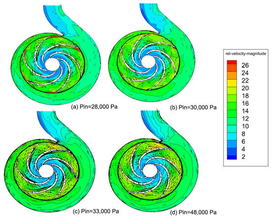
Figure 7.
Relative velocity distribution at different NPSHs.
4.5. Volume Fraction Distribution of Vacuoles in the Impeller Runner
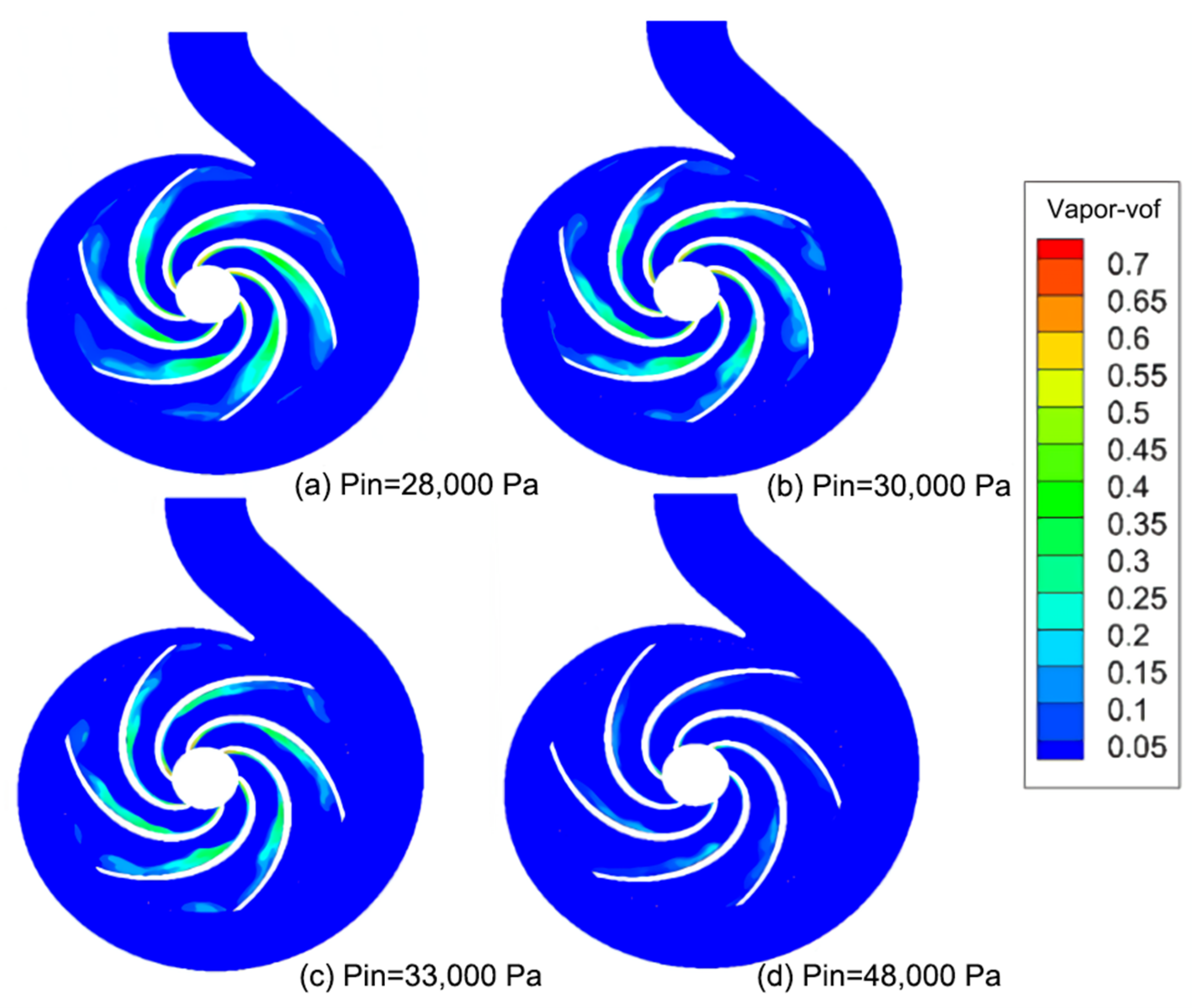
Figure 8 shows the impeller section’s cavitation volume fraction distribution at the designed flow rate. Figure 9 demonstrates the cavitation morphology. Figure 8d and Figure 9d show that when the pump’s effective cavitation margin is much higher than the critical cavitation margin, the cavitation phenomenon in the pump is not obvious, and only a small number of vacuoles are produced at the vane’s leading edge. Figure 8c and Figure 9c show that when the centrifugal pump’s inlet pressure decreases to 33,000 pa, the blade’s suction side at the impeller flow channel begins to grow along the impeller, with the attached air bubble covering about 1/4 of the blade’s suction-side surface. Because of the fluid medium, the air bubbles along the impeller flow channel and in the middle of the blade’s suction side converge, crowding the impeller runner and the blade’s trailing edge because of pressure changes and secondary reflux at the latter. Due to pressure changes and secondary reflux, the vacuole is continuously shed until its collapse. Figure 8a,b and Figure 9a,b show that when the effective centrifugal pump’s cavitation margin is lower than the critical cavitation margin, the cavitation phenomenon intensifies, and the blade’s suction-side surface thickens and increases the vacuole area, extending the vacuole tail to the blade’s expanding surface pressure, thereby further crowding the impeller runner and seriously affecting the centrifugal pump’s operational performance.

Figure 8.
Volume fraction distribution of different NPSH vacuoles.
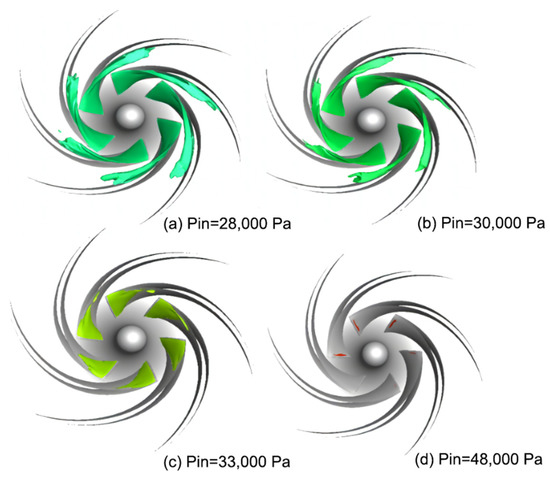
Figure 9.
Morphology of vacuoles under different NPSHs.
4.6. Blade Surface Load Distribution
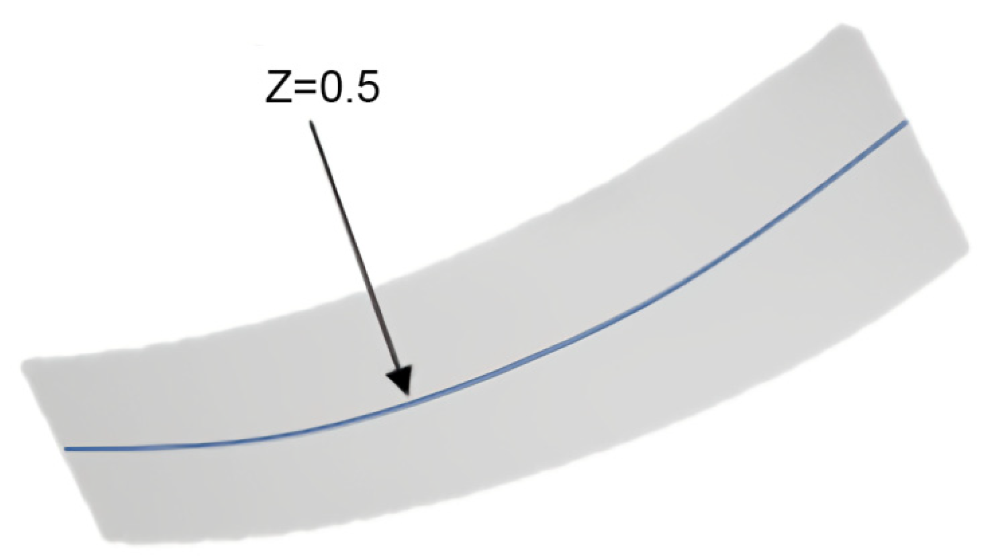
We demonstrated the impact of cavitation on the centrifugal pump’s operating performance by analyzing the load distribution at different degrees of cavitation on the vane’s pressure and suction surfaces. We selected the intersection line between any of the centrifugal pump’s vane surfaces and the impeller runner with a z = 0.5 rotational tangent (Figure 10).
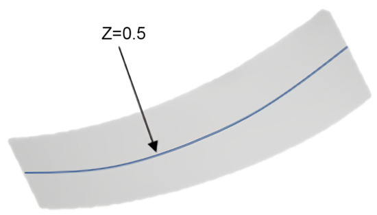
Figure 10.
Blade’s surface-pressure sampling curve.
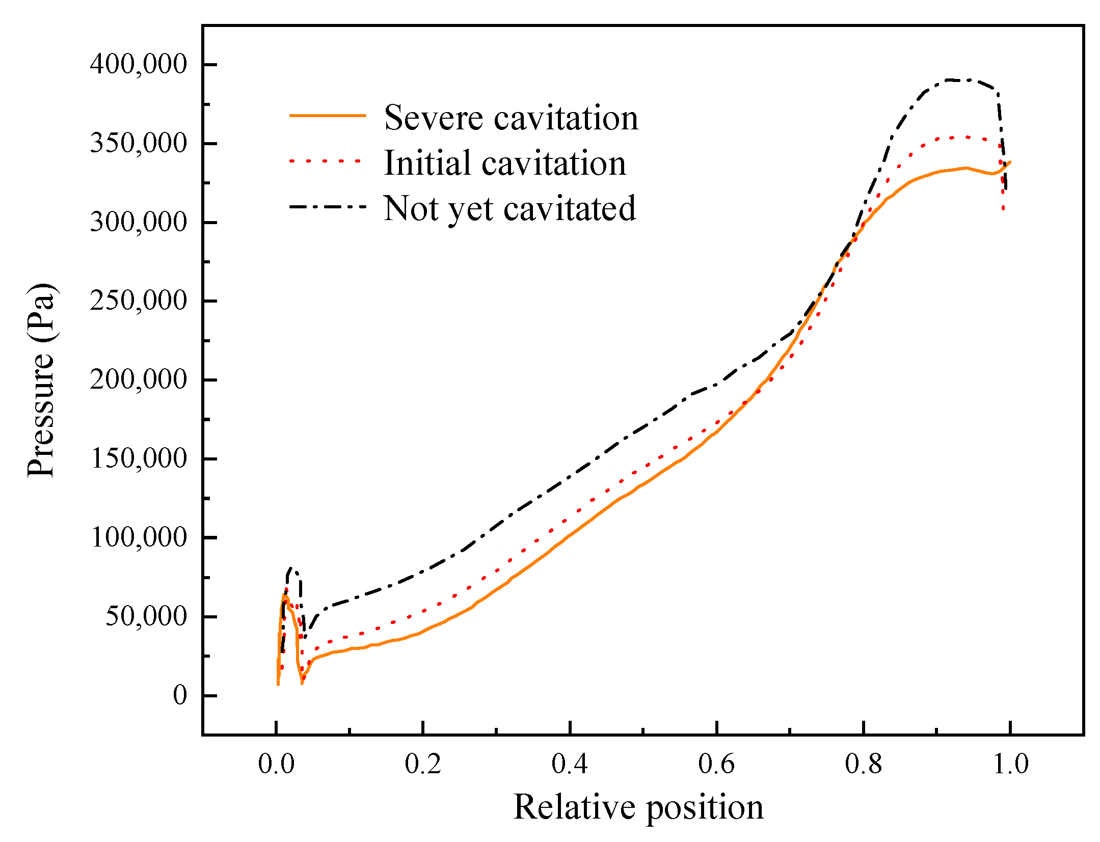
Figure 11 and Figure 12 show the blade’s surface-pressure and suction-surface load–distribution curves, respectively, and S is the 0~1 dimensionless number that characterizes the relative position of the blade’s surface. Figure 11 illustrates that the distribution trend of the blade’s surface-pressure load in various cavitation states is essentially comparable to the pressure load distribution along the relative position of the overall upward trend. The blade’s leading edge has a relatively small value point, meaning that the region easily produces cavitation phenomena. As the effective cavitation margin decreases, the blade’s load distribution generally shows a downward trend, and when the impeller runner displays serious cavitation, the very small value point of the blade’s leading edge is lower than the saturation steam pressure, indicating that there is a cavitation area.
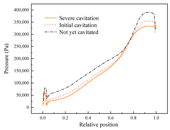
Figure 11.
Blade’s surface pressure–load distribution curve.

Figure 12.
Blade’s suction-surface load–distribution curve.
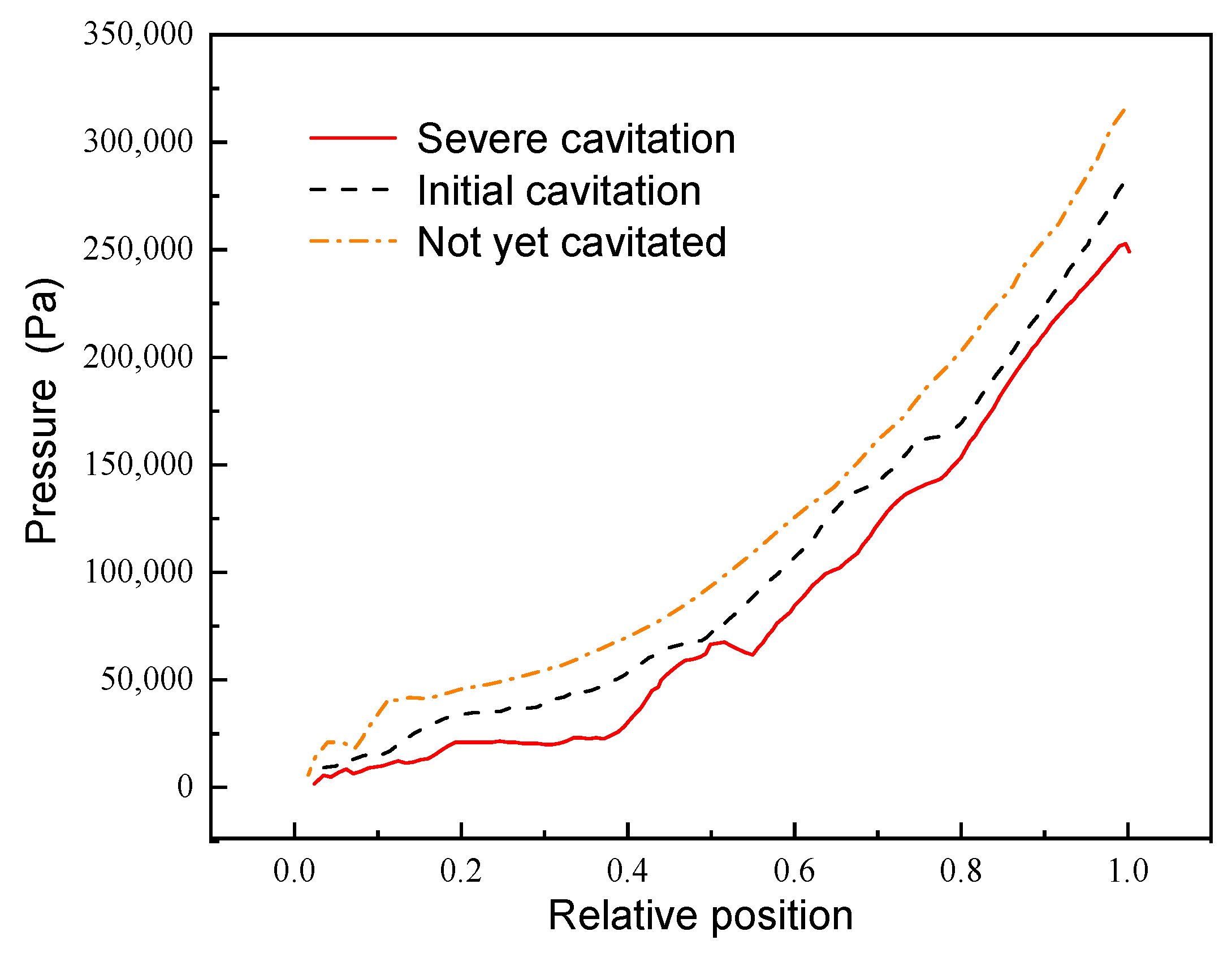
Figure 12 demonstrates that the vane’s suction-surface slope is greater than the vane’s surface-pressure slope, indicating that the vane’s suction-surface pressure–distribution gradient is greater. The blade’s suction surface’s low-pressure area is mainly concentrated in the vane’s leading edge position. Cavitation has not occurred, and the vane’s suction-surface curve is relatively smooth as a result of the residual reduction in effective cavitation, while the blade’s intermediate position appears at multiple extreme-pressure value points, due to the cavitation phenomenon expanding to the blade’s suction surface’s intermediate region. In this region, a large number of discrete small bubbles exist, which cause pressure curve fluctuations. The blade’s trailing edge in different cavitation-state curves is smoother, indicating a smaller influence of the cavitation phenomenon. Compared with Figure 11, the cavitation phenomenon primarily manifests at the blade’s suction side.
4.7. Impeller Runner Monitoring-Point Pressure-Pulsation Analysis
Figure 13 shows the arrangement of the pressure-pulsation monitoring sites. In our study, we set the pressure-pulsation monitoring points at two locations with obvious pressure-pulsation characteristics in the worm-shell flow channel; P1 is the worm-shell spacer, while P2 is the worm-shell-domain outlet. Unsteady-state calculations can be used to obtain the time-domain diagram of pressure pulsation at the pressure-pulsation monitoring locations. Because the pressure values are generally large, the pressure coefficient Cp is introduced to represent the transient pressure values. The expression of the pressure coefficient is as follows:
where p is the pressure value (Pa), ∆p is the average pressure value (Pa), ρ is the liquid density (kg/m3), and ν is the impeller outlet’s circumferential velocity (m/s).
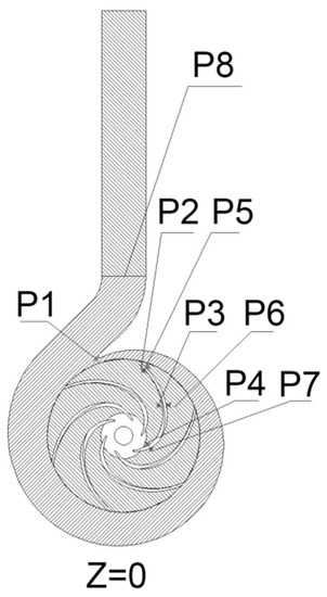
Figure 13.
Setting pressure-pulsation monitoring points.
To examine the centrifugal pump’s pressure-pulsation properties under various cavitation scenarios, we used the transient pressure values of the last three flow cycles at each monitoring point under three different cavitation states, and we obtained pressure coefficient frequency-domain maps after converting them into pressure coefficients and applying fast Fourier transform (FFT) to each monitoring point’s pressure coefficient time-domain data.
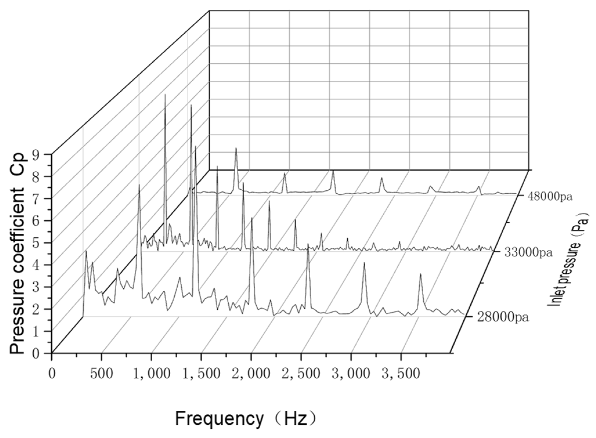
Figure 14 and Figure 15 show the frequency-domain plots of the pressure coefficients at the monitoring points of the worm-shell spacer and the worm-shell outlet, respectively. The frequency-domain diagrams of the pressure coefficients at the two monitoring points in different cavitation states are discrete, and the main frequency is the blade passage frequency ƒ = 293 Hz and its n times frequency. The two monitoring stations show a low-frequency pressure-pulsation signal when the cavitation event takes place in the flow channel, which creates a small amount of random pressure-pulsation signals. Figure 14 shows that with the deepening of the cavitation, the main frequency amplitude at the tongue shows a trend of increasing and then decreasing, and the n-frequency amplitude tends to increase, due to the enhancement of the flow field at the tongue after the cavitation has been disturbed. However, as a result of the drop in inlet pressure, the main frequency amplitude shows a small decrease. Figure 15 shows that with the deepening of the cavitation, the trends of frequency-domain changes at the outlet and the septum are similar—the main frequency amplitude increases and then decreases, and the n-frequency amplitude increases; however, the change in the main frequency amplitude at the outlet is less than that at the septum.
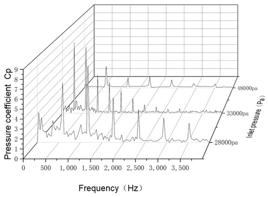
Figure 14.
Frequency-domain diagram of pressure pulsation across the tongue.
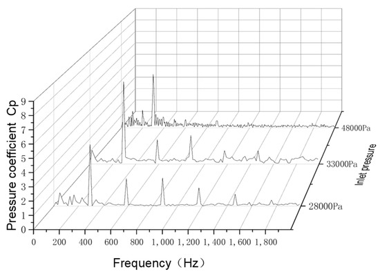
Figure 15.
Frequency-domain diagram of pressure pulsation at the volute outlet.
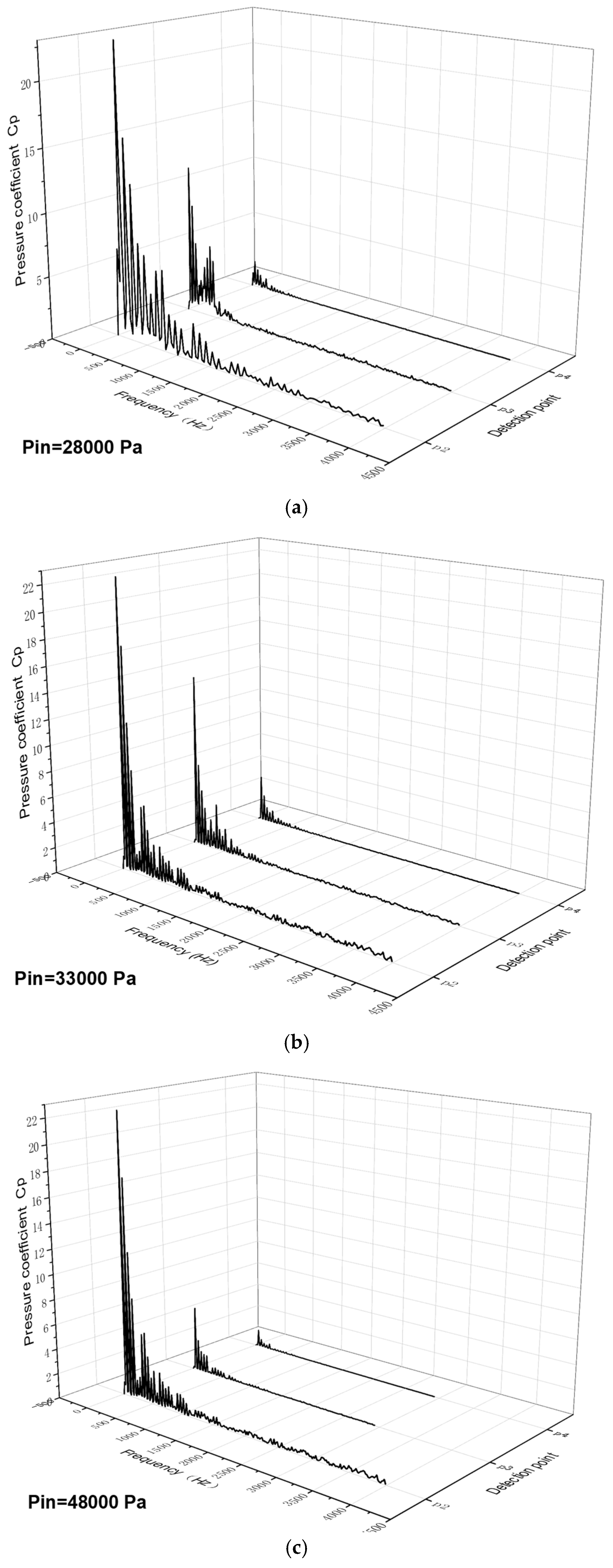
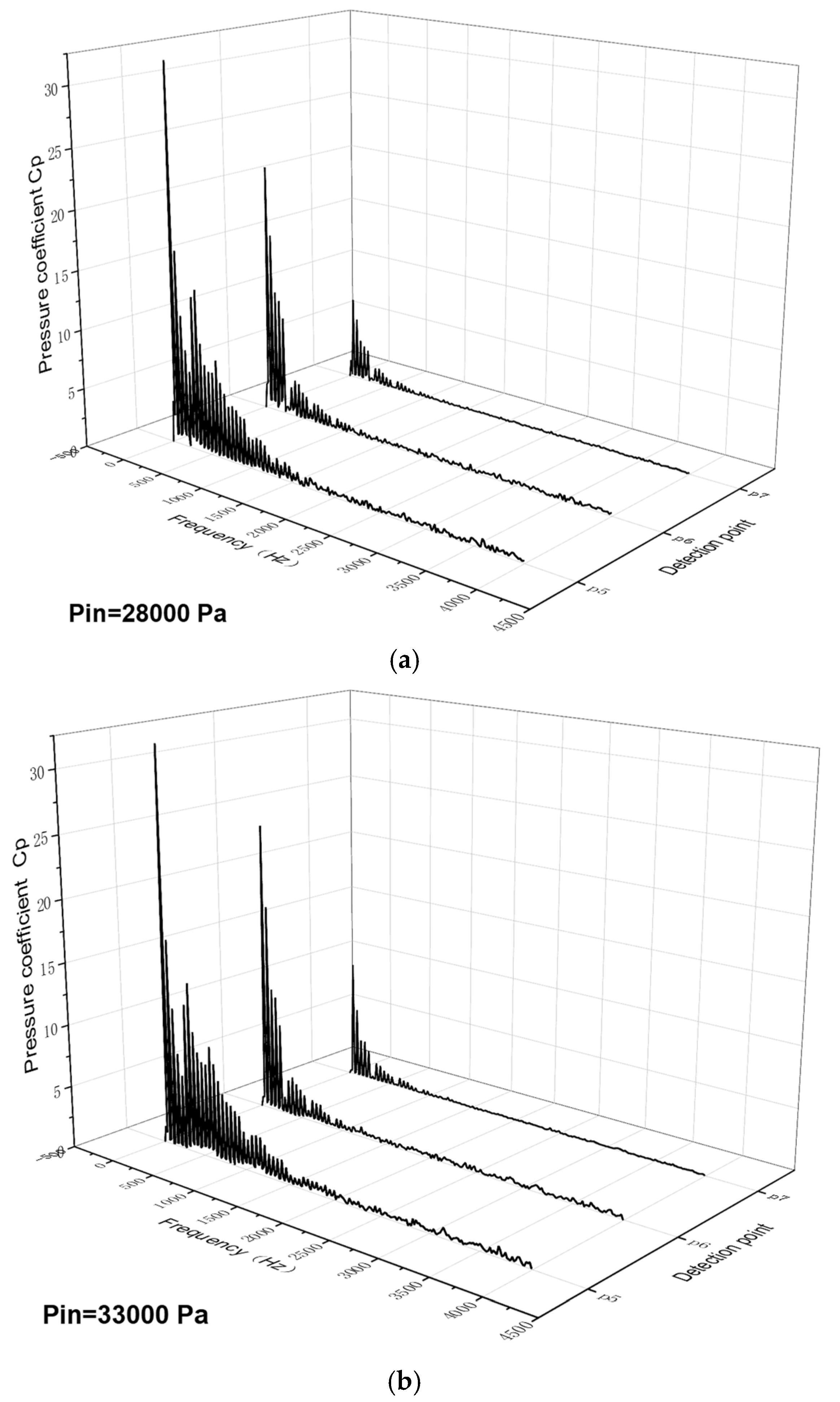
Figure 16 and Figure 17 show the frequency-domain waterfall plots of pressure pulsation at monitoring points P2~P7 in the impeller domain under three different cavitation states, where P2, P3, and P4 are the blade’s suction surface and P5, P6, and P7 are the blade’s surface pressure, respectively. Figure 17 shows that the main frequency amplitude steadily drops along the impeller runner at each monitoring station. The amplitude of the principal frequency at point P2 located at the leading edge of the blade is the highest among the three monitoring points, and the amplitude of the principal frequency at point P2 decreases with the deepening of the cavitation degree. The earliest connected vacuoles form on the blade’s suction surface’s leading edge, and the area with a higher vacuole volume fraction causes the main frequency amplitude to decrease, which may be due to the expansion of the vacuole area to the middle of the blade’s flow channel after the collapse of continuous shedding, resulting in an increase in the pulsation amplitude. With the intensification of cavitation, the vacuole area further extends, and the pulsation amplitude decreases. The changes to the blade’s trailing edge at P4 are relatively small compared with P2 and P3, indicating that the blade’s trailing edge at the impact of cavitation is the smallest. Figure 17 shows that when the cavitation intensifies, the three monitoring locations on the blade’s surface pressure display a modest drop in the main frequency amplitude, mainly due to the reduction in the inlet pressure.
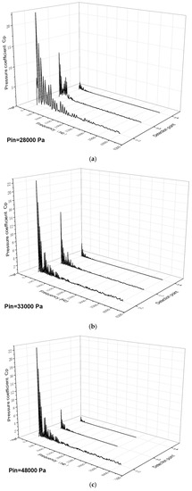
Figure 16.
(a–c) Frequency-domain diagram of pressure pulsation at the suction surface of the blade.

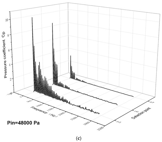
Figure 17.
(a–c) Frequency-domain diagram of pressure pulsation on the surface pressure of the blade.
5. Conclusions
We proposed a numerical calculation method to improve the ZGB cavitation model based on the rotational motion characteristics, considering the phenomenon that a certain size of vacuole will be torn into smaller-sized vacuoles in the impeller runner with high-speed rotation, while at the same time simulating the phenomenon of small fluctuations in rotational speed caused by hydrodynamic excitation force.
(1) When the improved ZGB cavitation model based on the rotational motion characteristics was applied to our numerical calculation of the centrifugal pump’s cavitation characteristics, the calculated cavitation performance curves were closer to the experimental values than the traditional ZGB model.
(2) Centrifugal pump cavitation was generated by air bubbles, which were mainly in the front edge of the blade’s suction. When the centrifugal pump’s cavitation degree intensified, air bubbles at the blade’s suction side began to grow along the impeller runner, with the air bubble area covering about 1/4 of the blade’s suction-side surface; air bubbles gathered along the impeller runner’s movement and in the middle of the blade’s suction side, crowding the impeller runner so that the pump’s running performance decreased considerably. Compared with the surface pressure, the blade’s suction surface was larger due to the cavitation phenomenon, while its pressure–load curve could be divided into a low-pressure cavitation area, a pressure fluctuation area, and a pressure stability area.
(3) The pressure–frequency-domain diagram of each monitoring point was a discrete distribution, and the main frequency was the blade’s passing frequency ƒ = 293 Hz and its n times frequency. With the deepening of the cavitation, the amplitude of the main frequency in the low-frequency band showed a trend of increasing and then decreasing, and the amplitude of the high-frequency band showed an increasing trend.
5.1. Innovation Points
The purpose of our paper was to study the test pump’s cavitation failure mechanism based on the fluid analysis software Fluent to numerically simulate the flow field inside the test pump’s cavitation, thereby improving the original ZGB cavitation and RNG k-ε turbulence models based on previous theories. We proposed a numerical calculation method to improve the ZGB cavitation model based on the rotational motion characteristics, considering that small fluctuations in rotational speed are caused by the action of hydraulic excitation forces within the impeller runner rotating at high speed. Then, with the help of our theoretical model, we studied the development process and internal flow-field characteristics of the test pump’s cavitation state to provide theoretical guidance for the acquisition of original vibration signals.
5.2. Computer Equipment
The server used for the numerical calculation of this subject had a higher computing power compared to a personal computer. Its processors were Intel(R) Xeon(R) Platinum 8373C CPU @ 2.60 GHz 2.60 GHz (two processors).
5.3. Research Perspectives
We mainly used Fluent numerical simulation to study a centrifugal pump’s cavitation characteristics. If conditions allow, the introduction of a visualization test combined with the simulation results for observation and comparison can more intuitively show the development process of a centrifugal pump’s cavitation state and internal flow-field characteristics. In turn, the theoretical model can be used to explore a centrifugal pump’s cavitation failure mechanisms and provide theoretical guidance to design a signal acquisition scheme.
Author Contributions
Conceptualization, J.W.; Formal analysis, J.W. and L.S.; Methodology, L.S.; Project administration, J.W. and Y.L.; Software, L.S.; Supervision, J.W. and Y.Z.; Validation, L.S., Y.Z., Y.L. and F.Z.; Visualization, Y.L. and F.Z.; Writing—original draft, L.S.; Writing—review & editing, J.W. All authors have read and agreed to the published version of the manuscript.
Funding
This research was funded by the Jiangsu Provincial Youth Fund (BK20201007) and the Jiangsu Provincial University Fund (20KJD470002).
Data Availability Statement
Data are contained within the article. All the code generated or used during the study are available from the corresponding author.
Acknowledgments
The author thanked the Jiangsu Provincial Youth Fund and Jiangsu Provincial Higher Education Fund.
Conflicts of Interest
The authors declare no conflict of interest.
Nomenclature
| ns | Specific speed |
| Q | Flow rate |
| H | Head |
| ne | Rotational speed |
| Z | Number of blades |
| k | Turbulent kinetic energy |
| ε | Turbulent dissipation rate |
| Gk | Turbulent kinetic energy generation term |
| Curvature correction coefficient | |
| ρv | Density of gas phase |
| Density of mixed homogeneous phase | |
| Density of liquid phase | |
| Nucleation volume fraction | |
| Evaporation coefficient | |
| Condensation coefficient | |
| Bubble radius | |
| Maximum vacuole radius | |
| Evaporation coefficient | |
| Ccond | Condensation coefficient |
| Time step | |
| n’ | Rotational speed in the previous time step |
| m | Previous time step’s output hydraulic torque |
| P | Shaft output power |
| Motor’s rotational inertia |
References
- Wang, F. Advances in computational modeling of rotational turbulence in fluid machinery. J. Agric. Mach. 2016, 47, 1–14. [Google Scholar]
- Gu, W.; He, Y.; Hu, T. Noise characteristics and bubble interface transients in axisymmetric body bubble flow. J. Shanghai Jiaotong Univ. 2000, 34, 1026–1030. [Google Scholar]
- Zhao, C.; Wang, C.; Wei, Y.; Zhang, X. Experiments on cavitation flow field and ballistic characteristics of slender body underwater motion. Explos. Impact 2017, 37, 439–446. [Google Scholar]
- Savar, M.; Kozmar, H.; Sutlovic, I. Improving centrifugal pump efficiency by impeller trimming. Desalination 2009, 249, 654–659. [Google Scholar] [CrossRef]
- Zhao, G. Research on Cavitation Flow Instability and Its Control in Centrifugal Pumps; Lanzhou University of Technology: Lanzhou, China, 2018. [Google Scholar]
- Li, Y.; Feng, G.; Li, X.; Si, Q.; Zhu, Z. An experimental study on the cavitation vibration characteristics of a centrifugal pump at normal flow rate. J. Mech. Sci. Technol. 2018, 32, 4711–4720. [Google Scholar] [CrossRef]
- Zhang, D.; Pan, D.; Shi, W.; Zhang, X. Numerical simulation of cavitation flow and its induced pressure pulsation in axial flow pumps. J. Huazhong Univ. Sci. Technol. (Nat. Sci. Ed.) 2014, 42, 34–38. [Google Scholar]
- Tseng, C.C.; Wang, L.J. Investigations of Empirical Coefficients of Cavitation and Turbulence Model Through Steady and Unsteady Turbulent Cavitating Flows. Comput. Fluids 2014, 103, 262–274. [Google Scholar] [CrossRef]
- Morgut, M.; Nobile, E.; Bilus, I. Comparison of Mass Transfer Models for the Numerical Prediction of Sheet Cavitation around a Hydrofoil. Multiph. Flow 2011, 37, 620–626. [Google Scholar] [CrossRef]
- Liu, H.; Wang, J.; Wang, Y.; Zhang, H.; Huang, H. Influence of the Empirical Coefficients of Cavitation Model on Predicting Cavitating Flow in Centrifugal Pump. Nav. Archit. Ocean Eng. 2014, 6, 119–131. [Google Scholar] [CrossRef]
- Stavropoulos-Vasilakis, E.; Kyriazis, N.; Jadidbonab, H.; Koukouvinis, P.; Gavaises, M. Review of Numerical Methodologies for Modeling Cavitation. Cavitation Bubble Dyn. 2021, 1–35. [Google Scholar] [CrossRef]
- Supponen, O.; Farhat, M.; Obreschkow, D. High-speed imaging of high pressures produced by cavitation bubbles. In Proceedings of the International Conference on High-Speed Imaging and Photonics 2018, Enschede, The Netherlands, 8–12 October 2018. [Google Scholar]
- Ghorbani, M.; Alcan, G.; Yilmaz, D.; Unel, M.; Kosar, A. Visualization and image processing of spray structure under the effect of cavitation phenomenon. J. Phys. Conf. 2015, 656, 012115. [Google Scholar] [CrossRef]
- Asuaje, M.; Bakir, F.; Kouidri, S.; Kenyery, F.; Rey, R. Numerical modelization of the flow in centrifugal pump: Volute influence in velocity and pressure fields. Int. J. Rotating Mach. 2005, 3, 244–255. [Google Scholar] [CrossRef]
- Li, X. Study on the Flow Mechanism of Supercavitation around Water Wings; Beijing University of Technology: Beijing, China, 2008. [Google Scholar]
- Yakhot, V.; Orszag, S.A. Renormalization group analysis of turbulence. i. Basic theory. J. Sci. Comput. 1986, 1, 3–51. [Google Scholar] [CrossRef]
- Spalart, P.R.; Shur, M. On the sensitization of turbulence models to rotation and curvature. Aerosp. Sci. Technol. 1997, 1, 297–302. [Google Scholar] [CrossRef]
- Minemura, K.; Murakami, M. A theoretical study on air bubble motion in a centrifugal pump impeller. J. Fluids Eng. 1980, 102, 446–453. [Google Scholar] [CrossRef]
- Murakami, M.; Minemura, K.; Takimoto, M. Effects of entrained air on the performance of centrifugal pumps under cavitating conditions. Trans. Jpn. Soc. Mech. 1980, 23, 1435–1442. [Google Scholar]
- Wang, J.; Wang, Y.; Liu, H. Rotating Corrected-Based Cavitation Model for a Centrifugal Pump. J. Fluids Eng. 2018, 140, 111301. [Google Scholar]
- Sun, H.; Yuan, S.; Luo, Y.; Guo, Y. Analysis of non-constant flow inside a centrifugal pump with the joint action of water and electricity. J. Drain. Irrig. Mach. Eng. 2016, 34, 122–127,150. [Google Scholar]
- Guo, Y. Study on the Non-Constant Characteristics of Centrifugal Pump Torque and Speed; Jiangsu University: Zhenjiang, China, 2017. [Google Scholar]


Disclaimer/Publisher’s Note: The statements, opinions and data contained in all publications are solely those of the individual author(s) and contributor(s) and not of MDPI and/or the editor(s). MDPI and/or the editor(s) disclaim responsibility for any injury to people or property resulting from any ideas, methods, instructions or products referred to in the content. |
© 2023 by the authors. Licensee MDPI, Basel, Switzerland. This article is an open access article distributed under the terms and conditions of the Creative Commons Attribution (CC BY) license (https://creativecommons.org/licenses/by/4.0/).