Enzymatic Hydrolysis of Complex Carbohydrates and the Mucus in a Mathematical Model of a Gut Reactor

Abstract

The human gut microbiota rely on complex carbohydrates for energy and growth, particularly dietary fiber and host-produced mucins. These complex carbohydrates must first be hydrolysed by certain microbial groups to enable cross-feeding by the gut microbial community. We consider a mathematical model of the enzymatic hydrolysis of complex carbohydrates into monomers by a microbial species. The resulting monomers are subsequently digested by the microbial species for growth. We first consider the microbial species in a single compartment continuous stirred-tank reactor where dietary fiber is the only available substrate. A two compartment configuration in which a side compartment connected by diffusion is also studied. The side compartment is taken to be the mucus layer of the human colon, providing refuge from washout and an additional source of complex carbohydrate in the form of mucins. The two models are studied using stability analysis, numerical exploration, and sensitivity analysis. The delay in substrate availability due to hydrolysis results in bistability and the unconditional asymptotic stability of the trivial equilibrium. The addition of the mucus compartment allows the microbial species to survive under conditions that would otherwise result in washout in a comparable single compartment reactor. This would suggest that depending on the features of the gut microbiota being studied, extracellular hydrolysis and a representation of the mucus layer should be included in mathematical and lab reactor models of the human gut microbiota.

1. Introduction

The human colon houses a complex community of microogranisms that have a significant impact on human health and disease. These microbes persist in part on complex carbohydrates that escape digestion in the upper gastrointestinal tract. The complex carbohydyrates, which primarily include resistant starches, plant cell wall polysaccharides and non-digestible oligosaccharides, are digested into beneficial metabolites by the microbial community once they reach the colon [1]. Though complex carbohydrates are the primary source of nutrients for the entire gut microbial community, their degradation must be initiated by a subset of the population referred to as the primary degraders [1,2]. This group of gut microbiota possess a suite of enzymes that break down complex carbohydrates into consumable sugars through the process of enzymatic hydrolysis [1]. We develop two mathematical models of the microbial-assisted enzymatic hydrolysis of complex carbohydrates into consumable sugars, and the growth of microbial species from the produced sugars, as a system of ordinary differential equations (ODEs). Our models are formulated in the context of a chemostat framework, mimicking experimental bioreactors that are often used to study questions of gut health. The carbohydrates are in the form of externally supplied dietary fiber, and, in the case of the second model, internally produced mucins which are sloughed from a mucus layer representation. We present a mathematical and computational analysis of the resulting ODE models. The aim of this work is to explore in greater detail the mechanism of the enzymatic hydrolysis of carbohydrates, to understand the impact of this process on mechanistic models of the gut, and to determine the importance of including a mucus representation in both mathematical and experimental reactor models of the gut.

The human colon is a tubular-shaped organ consisting of a hollow lumen covered with a two layer mucosal membrane. The mucus layer has many functions in the gut, including (i) being a physical barrier that separates the gut microbial from the host, (ii) providing attachment sites that prevent microbes from washout, and (iii) providing the gut microbiota with a source of carbon in the form of glycoproteins (mucins) [3]. Mucus is continuously shed into the lumen, allowing both luminal and mucosal bacteria to forage on glycoproteins. The mucosal community is thought to differ from the luminal community in composition, rate of proliferation and resource utilization [4,5]. While the composition of the colonic microbial community differs between individuals, in a healthy state, there exists a stable community that grants protective, structural and metabolic benefits to the host [6].

A key role of the gut microbiota is the fermentation of complex substrates that escape digestion in the upper gastrointestinal tract, the majority of which are insoluble complex carbohydrates. The degradation of these complex carbohydrates to soluble monomeric sugars results in the release of energy to the microbial community. This is facilitated by certain microbial species that have varying degrees of nutritional specialization and abundance. Endogenously produced mucins also serve as a major source of complex carbohydrates. In the absence of dietary fiber, such as during low fiber diets, members of the gut microbial community shift to the metabolism of mucus glycans [3]. This shift has been correlated with a compromised colonic mucus barrier and several negative health outcomes, such as imbalances in the gut microbial community (dysbiosis), increased pathogen susceptibility, and several disease states [3].

Complex organic materials often must be degraded into substrates that can be consumed by microorganisms. The microbiota that inhabit the colon can express enzymes that the host cannot, allowing for the degradation of resistant macronutrients entering the colon. While the gut microbial community exhibits a high degree of functional redundancy, a subset of the gut microbial community are responsible for the extracellular enzymatic degradation of complex carbohydrates. This primary degradation of complex carbohydrates makes nutrients available in the form of soluble monosaccharides that results in cross-feeding by other groups of bacteria.

It is possible to investigate the interactions of complex carbohydrates, gut microbiota, and the colonic mucus barrier through in vivo, in vitro, and in silico methods, each with its advantages and drawbacks. In vivo studies which involve human subjects provide the greatest biological significance but have ethical, economical and practical constraints. Human clinical studies have shown correlations between dietary fiber deprivation and mucus layer integrity, and other negative outcomes; however, human studies of the gut microbiota are subject to host interference and are typically limited to end-point measurements in the form of fecal samples [7]. Moreover, while healthy states of homeostasis exist [8], gut communities vary between individuals [6,7]. These factors make drawing conclusions on underlying mechanisms and processes difficult.

Many of the shortcomings of in vivo studies can be addressed using in vitro and ex vivo studies. On a finer scale, this includes culture-based cell models, organ culture, and microfluidic systems. The goal of these approaches are to study microbiota–host interactions. These studies can provide functional and mechanistic information such as the adherence of commensal and pathogenic cells to intestinal epithelial cells and human mucosa. However, culture-based cell models are limited to human and microbial cells that can be cultured in a laboratory. In organ culture, organoid traits are dependent on the individual they were extracted from, and microfluidic systems are expensive and do not allow for high-throughput experiments. These experiments are limited to addressing specific interactions, and a single model cannot encompass all the features of colon physiology and gut microbiology [9].

In vitro fermentation models, or experimental gut reactors, can also be used to study the human colon on a larger scale. These experimental models range from simple batch culture to complex continuous culture or ‘chemostat’ systems, and allow for the study of the gut microbial community without the complexity of the host physiology [6]. For example, the Simulator of the Human Intestinal Microbial Ecosystem (SHIME), is a multicompartment bioreactor that simulates the human gut [10]. In [11] an overview of existing experimental gut reactor models is presented. Experimental gut reactors are typically seeded from feces and reach an equilibrium (steady state) that resembles the in vivo distal colon microbial community [6]. Unlike other types of experimental studies of the gut, experimental gut reactor studies are highly reproducible, economical and allow for the culture of whole gut microbial communities [12]. It is also possible to represent the mucus, for example, by using mucin breads or a mucin-covered microcosm [9]. However, the equilibrium state of the gut microbial community can vary depending on the source of the inoculum and varies between individuals and temporally within an individual fecal donor. Variation in reactor conditions, lack of simulation of mucosal binding sites, and the lack of host selective pressures can also result in a discrepancy between the composition of a reactor microbial community and fecal inocula [6]. Experimental gut reactors are easier to model than the in vivo system. Mathematical modelling can be a useful tool to understand such experimental systems and their limitations.

There are several existing mechanistic mathematical models of fermentation in the human colon by the gut microbiota, each with varying degrees of detail. To our knowledge, the first complete metabolic model of the human colon was presented in [13]. In this model, the lumen and mucus environments of the colon are considered as a bioreactor and the processes within the colon are derived from mass balances of the metabolites and microbial groups involved. The proximal, distal and transverse regions of the luminal colon are each represented as a continuously stirred-tank reactor (CSTR) connected in series. Intestinal mucus is modelled as a separate compartment adjacent to each region of the colon, providing additional substrate with transport of microbes and substrates occurring between the mucus compartment and its respective luminal compartment. The microbial community is based on the well-established Anaerobic Digestion Model 1 (ADM1) [14], which is routinely used in modelling anaerobic bioreactors in wastewater and solid waste treatment. Similarly, the model presented in [15] is also based on ADM1, using a more simplified representation of the colon and multiple input substrates. The colon is represented as a single compartment CSTR and input substrates include carbohydrates, galactooligosaccharides, and proteins. Following ADM1, [13] use a functional representation of the gut microbiota based on the degraded substrate and metabolic pathways, dividing the gut microbiota into four major groups. Carbohydrates are the only substrate considered, as they are the majority of substrate entering the colon, and are hydrolysed by the biomass functional group at the top of the metabolic chain. This model was extended in [16,17]. In [16], the colon is represented as a single reactor without separate lumen and mucus compartments. The gut microbiota are divided into 10 functional groups, each with 10 strains with stochastically generated growth parameters. Multiple substrates are available for growth, with biomass growth from protein, non-starch polysaccharides, resistant starch and sugars. Biomass growth from multiple substrates is possible with substrate preferences, and substrates is directly utilized for growth, without a hydrolysis step. In [18], a software tool in R is presented, allowing for multiple reactor configurations, substrates, biomass functional groups, and metabolic pathways. In [17], the colon is represented as a continuous plug flow reactor with a fixed-medium of constant volume attached to the inner surface representing the intestinal mucus layer. Materials are well-mixed across a cross-sectional area and transported through the colon occurs with constant velocity. As in [13], carbohydrates are the only substrate that enter the colon from the upper gastrointestinal tract but meal times are approximated rather than a constant rate of input. Anaerobic digestion of carbohydrates follows from [13], excluding gaseous states. A software tool in C of this model is presented in [19]. In [20], a plug-flow model of the human colon is presented, with a focus on the impact of colon physiology on bacterial growth and composition. A hydrodynamic approach is taken and the flow rate is related to intestinal wall contractions and water absorption along the colon. The two dominant phyla, the Bacteroidetes and the Firmicutes, compose the modelled bacterial groups. Finally, in [21], the presented model includes a sophisticated representation of the mucus layer and its properties, with the same metabolic processes in [13], excluding gaseous states. In all mathematical models discussed, the main products of fermentation are short-chain fatty acids (SCFAs), with [13,15,17,20], including the absorption of metabolites by the host.

Mathematical models of primary degradation have been explored in several studies in the context of anaerobic digestion and microbial growth in a chemostat. A relevant chemostat model with an additional degradation step has been previously studied in [22]. In this model, a nutrient is supplied into a chemostat with a single species of microorganism. The nutrient must first be converted into a growth-limiting intermediate product by the microorganism before it can be consumed for growth. Both the conversion rate of the nutrient to intermediate product and the growth rate of the organism through consumption of the intermediate product are described as monotone response functions. In [22], it was demonstrated that the washout equilibrium is locally asymptotically stable, even if an asymptotically stable positive equilibrium point exists. This results in the survival of the organism being additionally dependent on the initial concentration of the species. If the initial concentration of the organism is too low, it will tend towards the washout equilibrium, even if a stable positive equilibrium exists. Moreover, unlike the standard chemostat in [23], depending on the monotone response function used, the existence of more than one positive equilibria is possible. For example, for a Monod response function, there exists two positive equilibria, with one equilibrium being an asymptotically stable node and the other an unstable saddle point. Unlike the standard chemostat model, the model outcomes depend on initial conditions in addition to certain parameters.

While the various mathematical models share a common goal of characterizing the digestion in the colon, not all include a description of a primary degradation of complex carbohydrates or a distinct mucus compartment. We study the effect of including these features in a single compartment chemostat model of primary degradation that is extended to include a lateral diffusive compartment, as first presented in [13]. Representing the mucus layer as a separate compartment allows us to capture its main features, such as the distinct ecological niche of the mucus and its function providing attachment sites that prevent washout. This reactor configuration was studied in detail in [24], where the growth of a single species from a single growth-limiting substrate was considered in a chemostat model with a second lateral diffusive compartment. In [24], the first compartment is a standard single species chemostat with a second compartment that is connected through lateral diffusion. As with the standard chemostat, there is a constant flow of growth-limiting substrate into the first compartment only. The substrate and microorganism can pass between the two compartments through diffusion, but there is no inflow or outflow from the second compartment. As with the standard chemostat, under certain conditions, the washout equilibrium is globally asymptotically stable; however, there is an additional condition for stability that is dependent on diffusion and compartment volume not present in the standard chemostat. If the two conditions for stability of the washout equilibrium are not met, then there exists a single asymptotically stable positive equilibrium. It was found that the addition of the lateral diffusive compartment allowed for the survival of the organism in cases that would typically result in extinction in the single compartment standard chemostat model. In particular, if the microorganism is removed from the reactor at a rate higher than the maximal growth rate, the lateral diffusive compartment can act as a refuge for microorganisms and allow for survival.

In a mathematical model of carbohydrate digestion in the gut presented in [25], it was found that the model outcome following antibiotic treatment depended on the survival of the bacterial functional group responsible for the primary degradation of supplied substrate. If concentration of this group was reduced below a threshold concentration by antibiotic treatment, the system would tend to washout and would not recover. To understand the mechanisms responsible for complete washout, we study a subset of the model presented in [25]. While the fermentation of carbohydrates by the gut microbiota is a multistep process, this study will focus on the first step in the metabolic network. We assume this step occurs in two stages: (1) the hydrolysis of a complex polysaccharide (fiber) into monomeric sugars and (2) the substrate-dependent growth of a microorganism through the consumption of the monomeric sugar. The first stage, hydrolysis, is modelled using Contois kinetics, as are used in previous mathematical models of the human gut [13,15,17,21], where the growth rate depends on both the concentration of the microorganism and the concentration of fiber. The second stage, the growth of the microbial community, is modelled using Monod kinetics, where the growth rate depends on the concentration of the substrate. We model these processes in two reactor representations, (i) a single compartment continuously-stirred tank reactor representing the lumen and (ii) with the inclusion of the mucus as separate compartment attached to the lumen.

2. Model Formulation

In this section, we introduce two mathematical models of carbohydrate degradation in the human colon and the microbial group responsible for the hydrolysis of the carbohydrate. In the first model, we consider only the lumen environment of the colon and the dietary fiber that reach the colon. The second model adds the mucus environment as well as host-secreted mucins, which act as an additional source of substrate.

2.1. Single Compartment Model

In the simplest form, the model consists of the fermentation of a dietary polysaccharide (fiber) to a monosaccharide (sugar) by a single bacterial species in a simple continuous stirred-tank reactor (CSTR), shown in Figure 1. There is a constant flow of media into and out of the reactor and the contents of the reactor are fully mixed. Fiber enters into the reactor at a constant rate and there is a constant outflow of fiber, sugar and biomass. Fiber is exogenously degraded by the bacteria into consumable sugar through enzymatic hydrolysis. The sugar made available through the degradation of fiber is the only growth-limiting substrate available for the bacteria to consume.

2.1.1. Basic Model Assumptions

A1

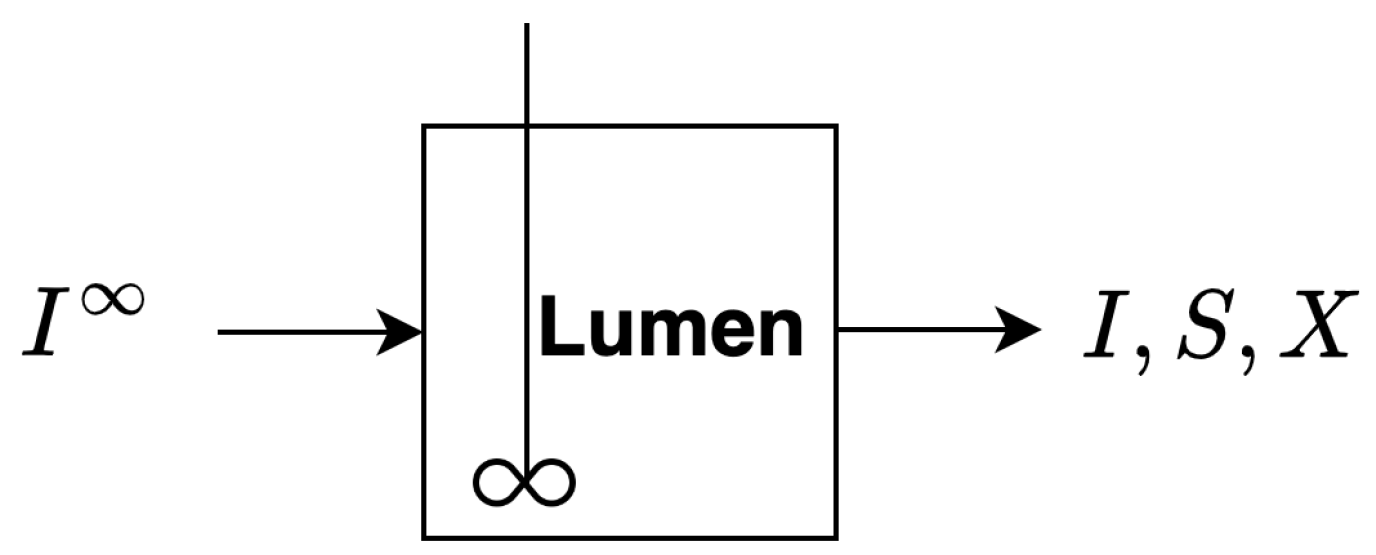
The reactor is fully mixed and contains fiber, sugar and bacteria. There is constant inflow of a fiber into the reactor and constant outflow of fiber, sugar and biomass from the reactor.

A2

Fiber is exogenously broken down into digestible monosaccharide sugar by the bacteria.

A3

Sugar is a growth limiting substrate consumed by the bacteria. The growth of bacteria is proportional to the uptake of sugar.

A4

Bacteria die through first-order decay.

2.1.2. Governing Equations

Based on the above assumptions, our model is formed in terms of the dependent variables: fiber concentration I [gL${}^{-1}$], sugar concentration S [gL${}^{-1}$] and sugar degrading biomass concentration X [gL${}^{-1}$].

$$\begin{array}{cc}\hfill & \dot{I}=\underset{\mathrm{A}1:\mathrm{Transport}}{\underbrace{D(I^{\infty }-I)}}-\underset{\mathrm{A}2:\mathrm{Hydrolysis}}{\underbrace{g(I,X)X}}\hfill \end{array}$$

(1)

$$\begin{array}{cc}\hfill & \dot{S}=\underset{\mathrm{A}1:\mathrm{Transport}}{\underbrace{-DS}}-\underset{\mathrm{A}3:\mathrm{Growth}}{\underbrace{f\left(S\right)X}}+\underset{\mathrm{A}2:\mathrm{Hydrolysis}}{\underbrace{Y_{I}g(I,X)X}}\hfill \end{array}$$

(2)

$$\begin{array}{cc}\hfill & \dot{X}=\underset{\mathrm{A}1:\mathrm{Transport}}{\underbrace{-DX}}+\underset{\mathrm{A}3:\mathrm{Growth}}{\underbrace{Y_{S}f\left(S\right)X}}-\underset{\mathrm{A}4:\mathrm{Decay}}{\underbrace{\alpha X}}\hfill \end{array}$$

(3)

The substrate dependent growth rate of X from S, $f\left(S\right)=\frac{{\kappa }_{S}S}{K_S+S}$, follows Monod kinetics. The rate of hydrolysis of I resulting in S, $g(I,X)=\frac{{\kappa }_{I}I}{K_{I}X+I}$, follows Contois kinetics. The dilution rate, D [d${}^{-1}$], is derived from $D=\frac{Q}{V}$, where Q [Ld${}^{-1}$] is the flow rate and V [L] is the reactor volume. ${\kappa }_I$ is the maximum specific hydrolysis rate of I to S. The parameter ${\kappa }_S$ [d${}^{-1}$] is the maximum specific growth rate of X from S and is achieved when S is in excess (ie. $S>>K_S$). The yield coefficients $Y_I$ [dimensionless] and $Y_S$ [dimensionless] are the yield of S per unit of I and X per unit of S, respectively. The parameters $K_I$ [dimensionless] and $K_S$ [gL${}^{-1}$] are half-saturation concentrations.

2.2. Dual Compartment Model

We extend the model presented in Section 2.1 to include the mucus environment of the human colon. The mucus environment is represented as a second compartment that is attached to the main luminal compartment. A schematic of the reactor configuration is shown in Figure 2. Mucins are endogenously produced in the mucus compartment and slough into the lumen. There is a transport of bacteria and sugar between the two compartments.

2.2.1. Basic Model Assumptions

A1

The reactor consists of two compartments of different volumes. Both reactor compartments are fully mixed and contain fiber, sugar and bacteria. The main compartment of the reactor represents the lumen of the colon. The second compartment of the reactor represents the mucus lining of the colon. There is constant inflow of a fiber into the lumen compartment and constant outflow of fiber, sugar and biomass from the lumen compartment. There is transport through the mucus compartment.

A2

Fiber is exogenously broken down into digestible monosaccharide sugar by the bacteria.

A3

Sugar is a growth limiting substrate consumed by the bacteria. The growth of bacteria is proportional to the uptake of sugar.

A4

Bacteria die through first-order decay.

A5

Mucins, which are analogous to fiber, are endogenously produced by the host in the mucus compartment.

A6

There is bi-directional exchange of all components between the lumen and mucus, excluding fiber. Mucins in the mucus compartment are sloughed into the lumen compartment, but there is no exchange of fiber from the lumen to the mucus compartment. Exchange is linear and donor-controlled.

2.2.2. Governing Equations

From the above assumptions, the model can be formed in terms of the dependent variables fiber concentration in the lumen $I_l$ [gL${}^{-1}$], sugar concentration in the lumen $S_l$ [gL${}^{-1}$], sugar degrading biomass concentration in the mucus $X_l$ [gL${}^{-1}$], fiber concentration in the mucus $I_m$ [gL${}^{-1}$], sugar concentration in the mucus $S_m$ [gL${}^{-1}$], and sugar degrading biomass concentration in the mucus $X_m$ [gL${}^{-1}$].

$$\begin{array}{cc}\hfill & {\dot{I}}_l=\underset{\mathrm{A}1:\mathrm{Transport}}{\underbrace{D(I^{\infty }-I_l)}}-\underset{\mathrm{A}2:\mathrm{Hydrolysis}}{\underbrace{g(I_l,X_l)X_l}}+\underset{\mathrm{A}6:\mathrm{Exchange}}{\underbrace{\left(\frac{V_m}{V_l}\right){\gamma }_{s,I}{I}_m}}\hfill \end{array}$$

(4)

$$\begin{array}{cc}\hfill & {\dot{S}}_l=\underset{\mathrm{A}1:\mathrm{Transport}}{\underbrace{-D{S}_l}}+\underset{\mathrm{A}2:\mathrm{Hydrolysis}}{\underbrace{Y_{I}g(I_l,X_l)X_l}}-\underset{\mathrm{A}3:\mathrm{Growth}}{\underbrace{f\left(S_l\right)X_l}}-\underset{\mathrm{A}6:\mathrm{Exchange}}{\underbrace{\frac{{\gamma }_d}{V_l}(S_l-S_m)}}\hfill \end{array}$$

(5)

$$\begin{array}{cc}\hfill & {\dot{X}}_l=\underset{\mathrm{A}1:\mathrm{Transport}}{\underbrace{-D{X}_l}}+\underset{\mathrm{A}3:\mathrm{Growth}}{\underbrace{Y_{S}f\left(S_l\right)X_l}}+\underset{\mathrm{A}6:\mathrm{Exchange}}{\underbrace{\left(\frac{V_m}{V_l}\right){\gamma }_{s,X}{X}_m}}-\underset{\mathrm{A}6:\mathrm{Exchange}}{\underbrace{{\gamma }_{a,X}{X}_l}}-\underset{\mathrm{A}4:\mathrm{Decay}}{\underbrace{\alpha X_l}}\hfill \end{array}$$

(6)

$$\begin{array}{cc}\hfill & {\dot{I}}_m=\underset{\mathrm{A}5:\mathrm{Mucin}}{\underbrace{\mathsf{\Lambda }\left(I_m\right)}}-\underset{\mathrm{A}2:\mathrm{Hydrolysis}}{\underbrace{g(I_m,X_m)X_m}}-\underset{\mathrm{A}6:\mathrm{Exchange}}{\underbrace{{\gamma }_{s,I}{I}_m}}\hfill \end{array}$$

(7)

$$\begin{array}{cc}\hfill & {\dot{S}}_m=\underset{\mathrm{A}2:\mathrm{Hydrolysis}}{\underbrace{Y_{I}g(I_m,X_m)X_m}}-\underset{\mathrm{A}3:\mathrm{Growth}}{\underbrace{f\left(S_m\right)X_m}}+\underset{\mathrm{A}6:\mathrm{Exchange}}{\underbrace{\frac{{\gamma }_d}{V_m}(S_l-S_m)}}\hfill \end{array}$$

(8)

$$\begin{array}{cc}\hfill & {\dot{X}}_m=\underset{\mathrm{A}3:\mathrm{Growth}}{\underbrace{Y_{S}f\left(S_m\right)X_m}}+\underset{\mathrm{A}6:\mathrm{Exchange}}{\underbrace{\left(\frac{V_l}{V_m}\right){\gamma }_{a,X}{X}_l}}-\underset{\mathrm{A}6:\mathrm{Exchange}}{\underbrace{{\gamma }_{s,X}{X}_m}}-\underset{\mathrm{A}4:\mathrm{Decay}}{\underbrace{\alpha X_m}}\hfill \end{array}$$

(9)

The substrate dependent growth rate of $X_i$ from $S_i$, $f\left(S_i\right)=\frac{{\kappa }_S{S}_i}{K_S+S_i}$, follows Monod kinetics where $i\in \{l,m\}$. The rate of hydrolysis of $S_i$ from $I_i$, $g(I_i,X_i)=\frac{{\kappa }_I{I}_i}{K_I{X}_i+I_i}$, follows Contois kinetics. D [d${}^{-1}$] is the dilution rate, from $D=\frac{Q}{V_l}$, where Q [Ld${}^{-1}$] is the flow rate and $V_l$ [L] is the volume of the lumen. ${\kappa }_I$ is the maximum specific hydrolysis rate of S from I. ${\kappa }_S$ [d${}^{-1}$] is the maximum specific growth rate of X from S and is achieved when S is in excess. The yield coefficients $Y_I$ [dimensionless] and $Y_S$ [dimensionless] are the yield of S per unit of I and X per unit of S, respectively. $K_I$ [dimensionless] and $K_S$ [gL${}^{-1}$] are half-saturation concentrations. $\mathsf{\Lambda }\left(I_m\right)$ [gL${}^{-1}$] is the concentration of endogenously produced mucin, the rate of production given below.

$$\begin{array}{ccc}\hfill \mathsf{\Lambda }=\left\{\begin{array}{cc}0,\hfill & \mathrm{if}\frac{I_m}{{\mathsf{\Gamma }}_{max}}>1\hfill \\ (1-\frac{I_m}{{\mathsf{\Gamma }}_{max}}){\mathsf{\Gamma }}_{prod},\hfill & \mathrm{otherwise}\hfill \end{array}\right.& \hfill & \hfill \end{array}$$

3. Model Analysis

3.1. Single Compartment Analysis

For use in local stability analysis, we calculate the Jacobian of Equations (1)–(3) as follows

$$J(I,S,X)=\left(\begin{array}{ccc}-D-g_I(I,X)X& 0& -[g(I,X)+g_X(I,X)X]\\ Y_I{g}_I(X,I)X& -D-f^{\prime }\left(S\right)X& Y_I[g_X(X,I)X+g(X,I)]-f\left(S\right)\\ 0& Y_S{f}^{\prime }\left(S\right)X& Y_{S}f\left(S\right)-D-\alpha \end{array}\right)$$

(10)

With

$$g(I,X):=\frac{{\kappa }_{I}I}{K_{I}X+I},f\left(S\right):=\frac{{\kappa }_{S}S}{K_S+S}$$

$$f^{\prime }\left(S\right)=\frac{{\kappa }_S{K}_S}{{(K_S+S)}^2},g_X(I,X)=-\frac{{\kappa }_I{K}_{I}I}{{(K_{I}X+I)}^2},g_I(I,X)=\frac{{\kappa }_I{K}_{I}X}{{(K_{I}X+I)}^2}$$

The Jacobian at a positive steady state is calculated as

$$J(I^{*},S^{*},X^{*})=\left(\begin{array}{ccc}-D-g_I(X,I)X& 0& -[g(I,X)+g_X(I,X)X]\\ Y_I{g}_I(X,I)X& -D-f^{\prime }\left(S\right)X& Y_I[g_X(X,I)X+g(X,I)]-\frac{D+\alpha }{Y_S}\\ 0& Y_S{f}^{\prime }\left(S\right)X& 0\end{array}\right)$$

(11)

Proposition 1. 

Models (1)–(3) preserves non-negativity. Solutions to the initial value problem are unique and exist for all time. Solutions depend continuously on model parameters and on initial data.

Proof. 

Positive invariance of the non-negative cone follows from the standard invariance theorem [26]. In the non-negative cone the right hand side is differentiable, thus a Lipschitz condition is satisfied. Thus, local existence and uniqueness of the initial value problem follow.

From non-negativity, it follows directly that $I\left(t\right)\le min\{I\left(0\right),I^{\infty }\}$. By comparison theorem it follows $X\left(t\right)\le X\left(0\right)exp({\kappa }_s{Y}_s-(D+\alpha ))$. From boundedness of $X\left(t\right)$ and $I\left(t\right)$ for any finite t it follows that $S\left(t\right)$ is bounded for any finite t. Thus, global existence follows. □

Proposition 2. 

The washout equilibrium $(I^{*},S^{*},X^{*})=(I^{\infty },0,0)$ is the only biomass free equilibrium. It exists for all choices of positive parameters. It is unconditionally asymptotically stable.

Proof. 

That for $X^{*}=0$ necessarily $I^{*}=I^{\infty }$ and $S^{*}=0$ is easily verified. We show local stability by linearisation. The Jacobian evaluated in the trivial equilibrium reads

$$J(I^{\infty },0,0)=\left(\begin{array}{ccc}-D& 0& *\\ 0& -D& *\\ 0& 0& -D-\alpha \end{array}\right)$$

(12)

where ∗ denotes a non-zero entry that depends only on parameters. Thus, all eigenvalues are negative, implying asymptotic stability. □

Proposition 3. 

Necessary for the existence of a nontrivial positive steady state $(I^{*},S^{*},X^{*})$ is

$$Y_S{\kappa }_s-(D-\alpha )>\frac{K_S(D+\alpha )}{Y_I{I}^{\infty }},$$

(13)

$$\frac{I^{\infty }{K}_I}{\frac{{\kappa }_I}{D}+{\kappa }_I}>I^{\infty }-\frac{K_S(D+\alpha )}{Y_I(Y_S{\kappa }_S-(D+\alpha ))}.$$

(14)

Proof. 

Note that in particular (13) implies also that $Y_S{\kappa }_s>D+\alpha$. For a steady state with $X^{*}>0$ and $S^{*}>0$ we need $Y_s{\kappa }_s{S}^{*}=(D+\alpha )(K_S+S^{*})$, thus $S^{*}=\frac{K_S(D+\alpha )}{Y_S{\kappa }_S-(D+\alpha )}$. This is the unique breakeven concentration for the population. For this to be positive, we require $Y_S{\kappa }_s>D+\alpha$.

With $S^{*}>0$ fixed, at steady state, we obtain two equations for $I^{*},X^{*}$, namely

$$0=-D{S}^{*}-\frac{{\kappa }_S{S}^{*}}{K_S+S^{*}}{X}^{*}+Y_I\frac{{\kappa }_I{I}^{*}}{K_I{X}^{*}+I^{*}}{X}^{*},0=D(I^{\infty }-I^{*})-\frac{{\kappa }_I{I}^{*}}{K_I{X}^{*}+I^{*}}{X}^{*}$$

(15)

Using the second of these and the expression for $S^{*}$, we obtain

$$0=-D{S}^{*}-\frac{{\kappa }_{S}S}{K_S+S^{*}}{X}^{*}+Y_{I}D(I^{\infty }-I^{*})$$

This simplifies to

$$Y_I{I}^{*}-\frac{D+\alpha }{D{Y}_S}{X}^{*}=Y_I{I}^{\infty }-S^{*}$$

(16)

which, due to positivity of $I^{*},X^{*}$ implies (13). Equation (16) defines a line segment in the positive cone of the I-X plane that connects the points $(0,Y_S\frac{D{S}^{*}}{Y_{I}D{I}^{\infty }})$ and $(I^{\infty }-\frac{S^{*}}{Y_I},0)$. The second equation of (15) rewrites as

$$0=I^{\infty }-I^{*}-\frac{{\kappa }_I}{D}\frac{I^{*}}{K_I{X}^{*}+I^{*}}{X}^{*}$$

$$0=(I^{\infty }-I^{*})(K_I{X}^{*}+I^{*})-\frac{{\kappa }_I}{D}{I}^{*}{X}^{*}$$

$$0=I^{\infty }{K}_I{X}^{*}+I^{\infty }{I}^{*}-{\left(I^{*}\right)}^2-\left(\frac{{\kappa }_I}{D}+K_I\right)I^{*}{X}^{*}$$

This finally defines the function

$$X^{*}=\frac{I^{\infty }{I}^{*}-{\left(I^{*}\right)}^2}{\left(\frac{{\kappa }_I}{D}+K_I\right)I^{*}-I^{\infty }{K}_I},$$

(17)

which has a singularity at

$${\widehat{I}}^{*}=\frac{I^{\infty }{K}_I}{\frac{{\kappa }_I}{D}+K_I}<I^{\infty }$$

A positive steady state is an intersection of the graph of (17) with (16). For $0<I^{*}<{\widehat{I}}^{*}$, (17) is negative. Thus if ${\widehat{I}}^{*}>I^{\infty }-\frac{S^{*}}{Y_I}$, no positive steady state can exist. This establishes (14). □

Proposition 4. 

Under the necessary conditions established in the previous proposition, there are at most two positive steady states, which can be explicitly calculated in terms of the model parameters only.

Proof. 

We continue with the calculations in the previous proof. Alternatively to (17), we can write

$$0={\left(I^{*}\right)}^2+\left[\left(\frac{{\kappa }_I}{D}+K_I\right)X^{*}-I^{\infty }\right]I^{*}-I^{\infty }{K}_I{X}^{*}$$

from which, upon substituting (16),

$$\begin{array}{cc}\hfill 0=& {\left(I^{*}\right)}^2+\left[\left(\frac{{\kappa }_I}{D}+K_I\right)\left(\frac{-D{Y}_S(Y_I{I}^{\infty }-Y_I{I}^{*}-S^{*})}{D+\alpha }\right)-I^{\infty }\right]I^{*}\hfill \\ \hfill & -I^{\infty }{K}_I\left(\frac{-D{Y}_S(Y_I{I}^{\infty }-Y_I{I}^{*}-S^{*})}{D+\alpha }\right)\hfill \end{array}$$

Thus, steady states are given by

$$S^{*}=\frac{D{K}_S}{Y_S{\kappa }_s-D}$$

(18)

and

$$\begin{array}{cc}\hfill I_{1,2}^{*}& =-\frac{1}{2}\left[\left(\frac{{\kappa }_I}{D}+K_I\right)\left(\frac{-D{Y}_S(Y_I{I}^{\infty }-Y_I{I}^{*}-S^{*})}{D+\alpha }\right)-I^{\infty }\right]\hfill \\ \hfill & \pm \frac{1}{2}\{{\left[\left(\frac{{\kappa }_I}{D}+K_I\right)\left(\frac{-D{Y}_S(Y_I{I}^{\infty }-Y_I{I}^{*}-S^{*})}{D+\alpha }\right)-I^{\infty }\right]}^2\hfill \\ \hfill & -4\left[I^{\infty }{K}_I\left(\frac{-D{Y}_S(Y_I{I}^{\infty }-Y_I{I}^{*}-S^{*})}{D+\alpha }\right)\right]{\}}^{1/2}\hfill \end{array}$$

(19)

and

$$X_{1,2}^{*}=\frac{-D{Y}_S(Y_I{I}^{\infty }-Y_I{I}^{*}-S^{*})}{D+\alpha }.$$

(20)

These are admissible if positive. □

3.2. Dual Compartment Analysis

For use in local stability analysis, the Jacobian of Equations (4)–(9) is as follows

$$J(I_l,S_l,X_l,I_m,S_m,X_m)=\left(\begin{array}{cc}A& B\\ C& D\end{array}\right),$$

(21)

where

$$\begin{array}{cc}\hfill & A=\left(\begin{array}{ccc}-D-g_{I_l}(I_l,X_l)X_l& -D-f^{\prime }\left(S_l\right)X_l-\frac{{\gamma }_d}{V_l}{S}_l& -g(I_l,X_l)-g_{X_l}(I_l,X_l)X_l\\ Y_I{g}_{I_l}(I_l,X_l)X_l& 0& 0\\ 0& Y_S{f}^{\prime }\left(S_l\right)X_l& -D+Y_{S}f\left(S_l\right)-{\gamma }_{a,X}-\alpha \end{array}\right)\hfill \\ \hfill & B=\left(\begin{array}{ccc}\frac{V_m}{V_l}{\gamma }_{s,I}& 0& 0\\ 0& \frac{{\gamma }_d}{V_l}& 0\\ 0& 0& \frac{V_m}{V_l}{\gamma }_{s,X}\end{array}\right)\hfill \\ \hfill & C=\left(\begin{array}{ccc}0& 0& 0\\ 0& \frac{{\gamma }_d}{V_m}& 0\\ 0& 0& \frac{V_l}{V_m}{\gamma }_{a,X}\end{array}\right)\hfill \\ \hfill & D=\left(\begin{array}{ccc}{\mathsf{\Lambda }}^{\prime }\left(I_m\right)-g_{I_m}(I_m,X_m)X_m-{\gamma }_{s,I}& 0& -g_{X_m}(I_m,X_m)X_m-g(I_m,X_m)\\ Y_I{g}_{I_m}(I_m,X_m)X_m& -f^{\prime }\left(S_m\right)-\frac{{\gamma }_d}{V_m}& Y_I{g}_{X_m}(I_m,X_m)X_m\\ & & +Y_{I}g(I_m,X_m)-f\left(S_m\right)\\ 0& Y_S{f}^{\prime }\left(S_m\right)X_m& Y_{S}f\left(S_m\right)-{\gamma }_{s,X}-\alpha \end{array}\right)\hfill \end{array}$$

With

$$\begin{array}{cc}\hfill & g(X,I):=\frac{{\kappa }_{I}I}{K_{I}X+I},f\left(S\right):=\frac{{\kappa }_{S}S}{K_S+S}\hfill \\ \hfill & g_{X{}_l}(I_l,X_l)=-\frac{{\kappa }_I{K}_I{I}_l}{{(K_I{X}_l+I_l)}^2},g_{I_l}(I_l,X_l)=\frac{{\kappa }_I{K}_I{I}_l{X}_l}{{(K_I{X}_l+I_l)}^2}\hfill \\ \hfill & g_{X_m}(I_m,X_m)=-\frac{{\kappa }_I{K}_I{I}_m}{{(K_I{X}_m+I_m)}^2},g_{I_m}(I_m,X_m)=\frac{{\kappa }_I{K}_I{I}_m{X}_m}{{(K_I{X}_m+I_m)}^2}\hfill \end{array}$$

Proposition 5. 

The washout equilibrium $(I_l^{*},S_l^{*},X_l^{*},I_m^{*},S_m^{*},X_m^{*})=(I^{\infty },0,0,I_m^{*},0,0)$ is the only biomass free equilibrium. It exists for all choices of positive parameters. It is unconditionally asymptotically stable.

Proof. 

The washout equilibrium $(I_l^{*},S_l^{*},X_l^{*},I_m^{*},S_m^{*},X_m^{*})=(I^{\infty },0,0,I_m^{*},0,0)$ can be calculated using standard techniques and setting Equations (4)–(9) to zero.

We show local stability by linearisation. The Jacobian evaluated at the trivial equilibrium is as follows

$$\begin{array}{cc}\hfill & J(I^{\infty },0,0,I_m^{*},0,0)=\hfill \end{array}$$

(22)

$$\begin{array}{cc}\hfill & \left(\begin{array}{cccccc}-D& 0& -{\kappa }_I& \frac{V_m}{V_l}{\gamma }_{s,I}& 0& 0\\ 0& -D& Y{}_I{\kappa }_I& 0& \frac{{\gamma }_d}{V_l}& 0\\ 0& 0& -D-{\gamma }_{a,X}-\alpha & 0& 0& \frac{V_m}{V_l}{\gamma }_{s,X}\\ 0& 0& 0& {\mathsf{\Lambda }}^{\prime }\left(I_m^{*}\right)-{\gamma }_{s,I}& 0& -{\kappa }_I\\ 0& \frac{{\gamma }_d}{V_m}& 0& 0& -\frac{{\kappa }_S}{{K_S}^2}-\frac{{\gamma }_d}{V_m}& Y_I{\kappa }_I\\ 0& 0& \frac{V_l}{V_m}{\gamma }_{a,X}& 0& 0& -{\gamma }_{s,X}-\alpha \end{array}\right)\hfill \end{array}$$

(23)

The eigenvalues can be calculated using standard techniques by finding the roots of the characteristic polynomial of $J(I^{\infty },0,0,I_m^{*},0,0)$.

$$\begin{array}{cc}\hfill {\lambda }_1& =-D\hfill \end{array}$$

(24)

$$\begin{array}{cc}\hfill {\lambda }_2& ={\mathsf{\Lambda }}^{\prime }-{\gamma }_{s,I}\hfill \end{array}$$

(25)

$$\begin{array}{cc}\hfill {\lambda }_{3,4}& =\frac{-(D+\frac{{\gamma }_d}{V_m}+\frac{k_s}{K_s^2})\pm \sqrt{{(D+\frac{{\gamma }_d}{V_m}+\frac{k_s}{{K_s}^2})}^2-4(\frac{D{k}_s}{{K_s}^2}+\frac{D{\gamma }_d}{V_m}+\frac{{\gamma }_d^2}{V_m{V}_l}})}{2}\hfill \end{array}$$

(26)

$$\begin{array}{cc}\hfill {\lambda }_{5,6}& =\frac{-(D+{\gamma }_{a,X}+{\gamma }_{s,X}+2\alpha )}{2}\hfill \end{array}$$

(27)

$$\begin{array}{cc}\hfill & \pm \frac{{\left[{(D+{\gamma }_{a,X}+{\gamma }_{s,X}+2\alpha )}^2-4(D{\gamma }_{s,X}+D\alpha -{\gamma }_{a,X}\alpha +{\gamma }_{s,X}\alpha +{\alpha }^2)\right]}^{1/2}}{2}\hfill \end{array}$$

(28)

For positive parameters, ${\lambda }_1$, ${\lambda }_{3,4}$, and ${\lambda }_{5,6}$ have negative real parts. In ${\lambda }_2$, for all positive parameters, ${\mathsf{\Lambda }}^{\prime }$ is zero or negative, resulting in ${\lambda }_2<0$. □

4. Numerical Results

We perform a simulation study of the equations presented in Section 2.1.2 and Section 2.2.2 to validate and augment the analytical results presented in Section 2.1.2. Our analytical results demonstrate that it is possible for two possible stable equilibria to exist. Our numerical analysis confirms these results and further demonstrates the bistability of the system and its dependence on initial conditions.

The systems of ODEs presented in Section 2.1.2 and Section 2.2.2 was solved using the ODE solver solve_ivp as implemented in SciPy; all simulations were conducted using Python 3.8. The model and simulation experiments are determinisitic and depend on model parameters. Simulations were run until the concentrations of I, S, and X reached steady state. Steady state was assumed to be reached when the 2-norm of the RHS was less than $ϵ$, where $ϵ={10}^{-3}$.

4.1. Single Compartment

For the following simulations in the single compartment configuration, the parameter values given in

Table 1. Mean values of parameters used in numerical simulations of single compartment model, adapted from [17].

Parameter	Symbol	Default Value	Unit
Death rate	$\alpha$	0.1	[gL${}^{-1}$]
Dilution rate	D	1.007	[d${}^{-1}$]
Inflow fiber concentration	$I^{\infty }$	1.0	[gL${}^{-1}$]
Max specific growth rate of X from S	${\kappa }_S$	12.627	[d${}^{-1}$]
Max specific hydrolysis rate	${\kappa }_I$	10.619	[d${}^{-1}$]
Half-saturation coefficient for growth of X	$K_S$	0.468	[gL${}^{-1}$]
Half-saturation coefficient	$K_I$	0.265	dimensionless
Yield coefficient for X using S	$Y_S$	0.342	dimensionless
Yield coefficient for hydrolysis	$Y_I$	1.0	dimensionless

were used unless otherwise specified. These values were adapted from the mathematical model presented in [17], and were originally derived from experimental gut reactor studies. In Section 4.1.1, the dilution rate D and the inflow fiber concentration $I^{\infty }$ were varied to show that enough nutrients must be available for growth for the microorganism to survive washout, as in the standard chemostat model. Unlike the standard chemostat model, the outcome can also depend on the initial concentration of biomass ($X_0$).

4.1.1. Typical Simulations

In typical simulations, two possible outcomes were observed once the system reached steady state: the washout of the microbial species or the persistence of the microbial species in the chemostat at a steady state concentration. As in the standard single species chemostat model, whether the microbial species survives depends on parameter values, as shown in Figure 3a,b. In Figure 3a, there is a critical value of $D=D_c$ such that if $D>D_c$, the growth rate is not sufficiently large and washout of the microbial species occurs. A similar result in shown in Figure 3b, where there is a critical inflow fiber concentration, below which washout occurs.

In Figure 3c, we can observe the single compartment model, described by Equations (1)–(3), is bistable. It is possible for two stable equilibrium states to exist for a fixed set of parameters, and the system trajectory depends on the initial biomass concentration, $X_0$. From Proposition 2, the washout equilibrium is attracting even if a stable positive equilibrium exists. The initial concentration of biomass must be greater than a threshold value in order for the system to tend to the positive equilibrium.

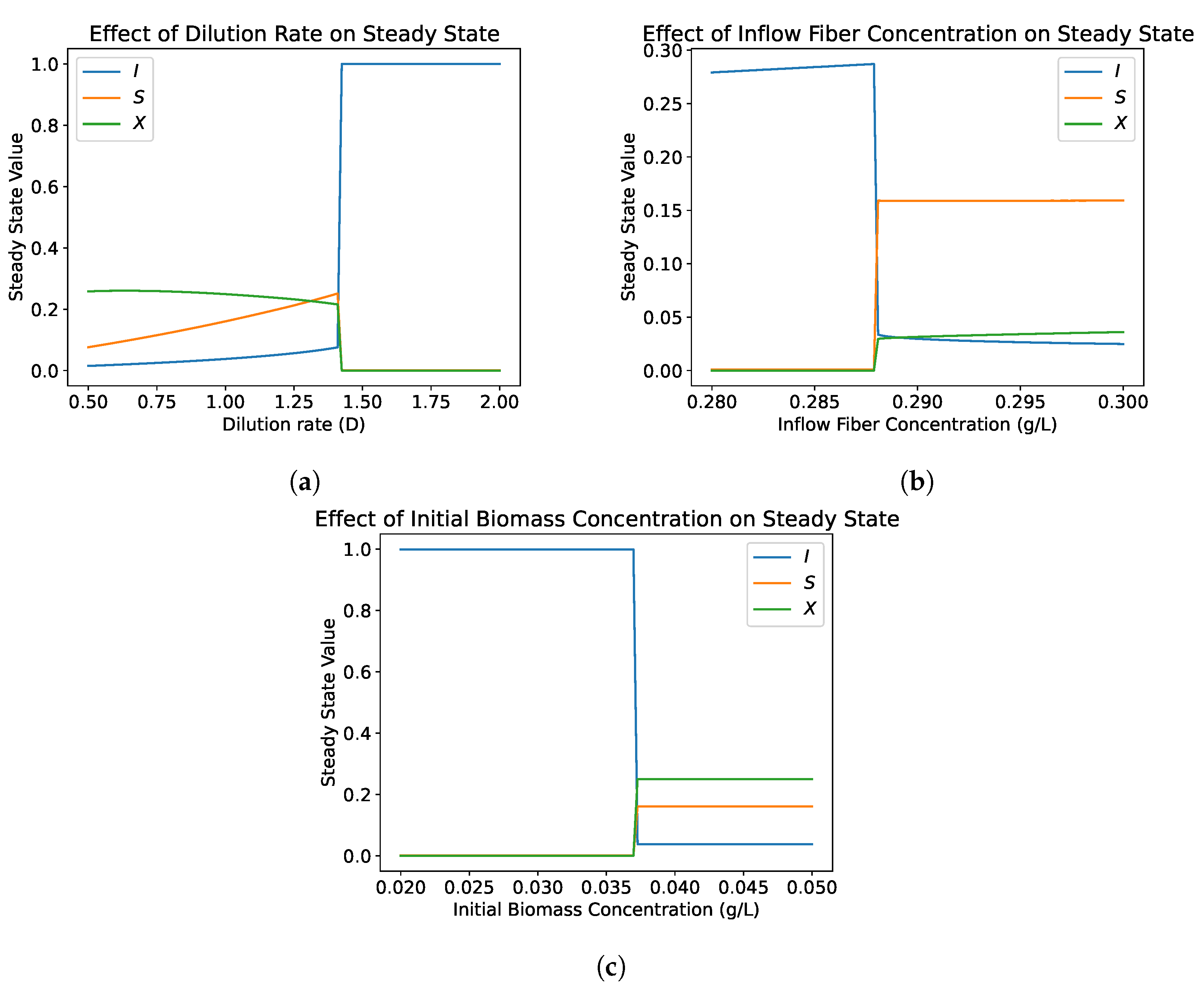
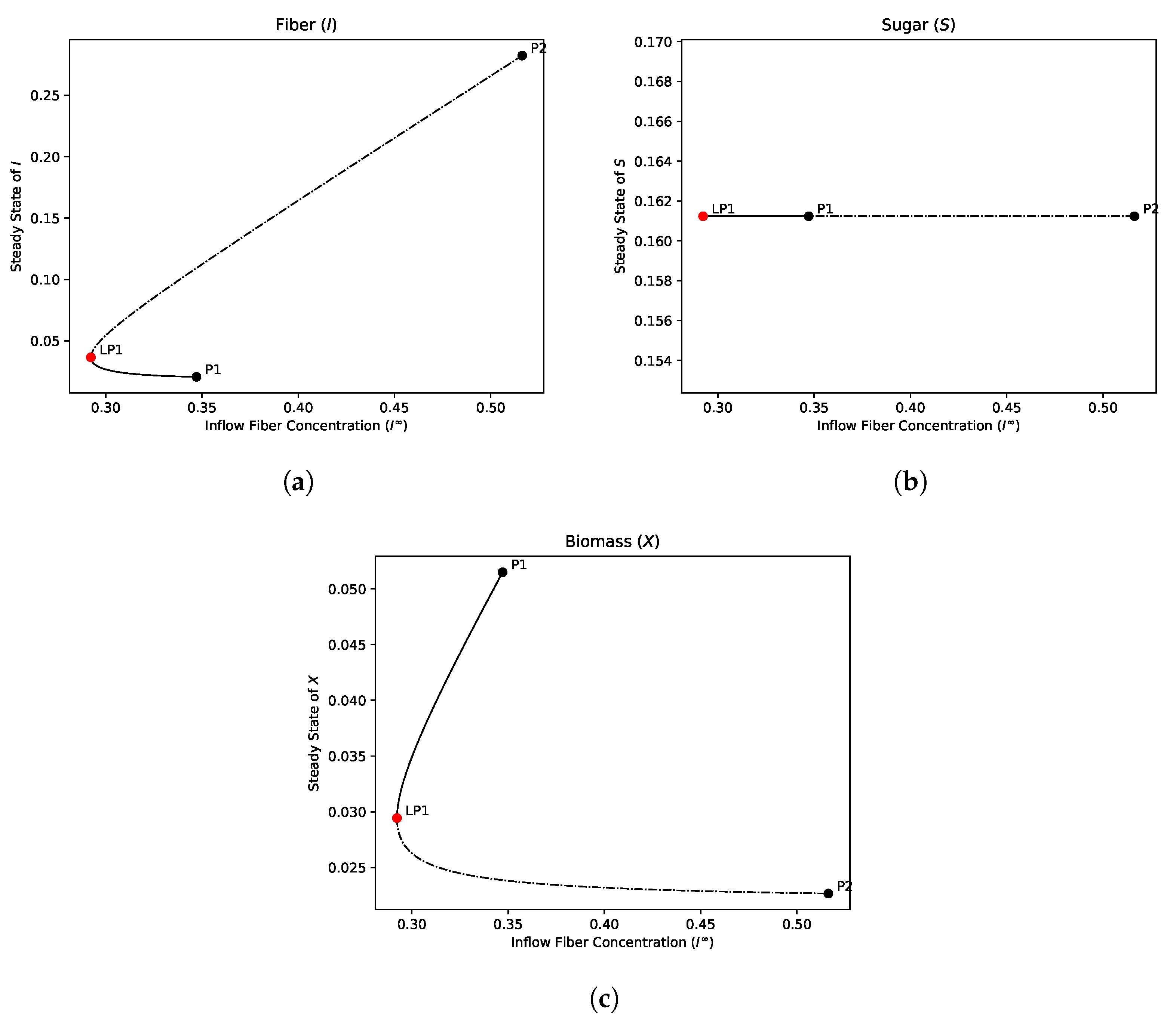
4.1.2. Bifurcation Analysis

The results shown in Figure 3c were further investigated using numerical continuation software. The PyCont sub-package of PyDSTool was used to produce the bifurcation diagrams in this section. In Figure 4a–c, the steady states of the single compartment model (Equations (1)–(3)) are plotted as a function of $I^{\infty }$. When $I^{\infty }$ is sufficiently large to satisfy the conditions for existence of a nontrivial positive steady state given in Proposition 4, two positive steady states emerge (i.e., when the discriminant in Equation (19) is greater than zero). $I_{1,2}^{*}$ and $X_{1,2}^{*}$, are calculated in Section 3.1 as Equations (17), (19), respectively, with one stable (solid line) and one unstable (dotted line) steady state. $S_{1,2}^{*}$ given in Equation (18), is independent of $I^{\infty }$ and takes the same value for both positive equilibria, if they exist.

4.2. Dual Compartment

Numerical simulations were conducted to investigate the role of the mucus compartment and the rate of transfer between the lumen and mucus compartment. Default parameter values from

Table 2. Default parameters used in numerical simulations for dual compartment model, adapted from [17].

Parameter	Symbol	Default Value	Units
Death rate	$\alpha$	0.1	[gL${}^{-1}$]
Dilution rate	D	1.007	[d${}^{-1}$]
Inflow fiber concentration	$I^{\infty }$	1.0	[gL${}^{-1}$]
Max specific growth rate of X from S	${\kappa }_S$	12.627	[d${}^{-1}$]
Max specific hydrolysis rate	${\kappa }_I$	10.619	[d${}^{-1}$]
Half-saturation coefficient for growth of X	$K_S$	0.468	[gL${}^{-1}$]
Half-saturation coefficient	$K_I$	0.265	dimensionless
Yield coefficient for X using S	$Y_S$	0.342	dimensionless
Yield coefficient for hydrolysis	$Y_I$	1.0	dimensionless
Diffusion rate	${\gamma }_d$	3.9	[Ld${}^{-1}$]
Attachment rate of X (Lumen to mucus)	${\gamma }_{a,X}$	0.1	[Ld${}^{-1}$]
Sloughing rate of I (Mucus to lumen)	${\gamma }_{s,I}$	0.1	[Ld${}^{-1}$]
Sloughing rate of X (Mucus to lumen)	${\gamma }_{s,X}$	0.4	[Ld${}^{-1}$]
Maximum mucus amount	${\mathsf{\Gamma }}_{max}$	500.0	[gL${}^{-1}$]
Mucus production rate	${\mathsf{\Gamma }}_{prod}$	50.0	[g(Ld)${}^{-1}$]
Volume of lumen	$V_l$	1.0	[L]
Volume of mucus	$V_m$	1.0	[L]

were used unless otherwise specified. In Section 4.2.1, we can observe that the bistability and dependence on initial biomass concentration ($X_0$) observed in the single compartment model (Figure 3c) can also be observed in the dual compartment model. In Section 4.2.2, simulations are conducted to investigate the influence of the mucus compartment and to determine if there is an optimal mucus volume for biomass survival. In Section 4.2.3, the rate of attachment of biomass from the lumen to mucus (${\gamma }_{a,X}$) and the rate of sloughing of biomass from the mucus to the lumen (${\gamma }_{s,X}$) are independently varied to determine their role in model outcomes and biomass concentrations at a steady state.

The parameters used in the numerical simulations and as the mean values in the sensitivity analysis are given below. The values were adapted from the gut model presented in [17], which were originally derived from experimental gut reactor studies.

4.2.1. Typical Simulations

As in the single compartment model, the hydrolysis of fiber results in a dependence on the initial concentration of biomass for survival due to the stability of the trivial equilibrium from Proposition 5. In Figure 5, once the initial concentration reaches a threshold, the system transitions from the stable trivial equilibrium to a stable positive equilibrium.

4.2.2. Role of Mucus Compartment

Simulations were conducted to investigate how the ratio of lumen and mucus volume affect the survival of the biomass (Figure 6a). The total reactor volume was held constant between simulations (i.e. $V_l+V_m=1.0$L). In the single compartment model (i.e., $V_l=1.0$L and $V_m=0.0$L), this parameter set and initial conditions would result in the eradication of the biomass. The addition of the mucus compartment can prevent the washout of the biomass species from occurring. As shown in Figure 6a, there is an optimal mucus volume that allows for survival of the biomass. If the mucus volume is too small or too large relative to the lumen volume of the reactor, the microbial species does not survive. For intermediate values of mucus volume, which correspond to biological relevant mucus/lumen ratios, the mucus compartment can act as a refuge for the biomass.

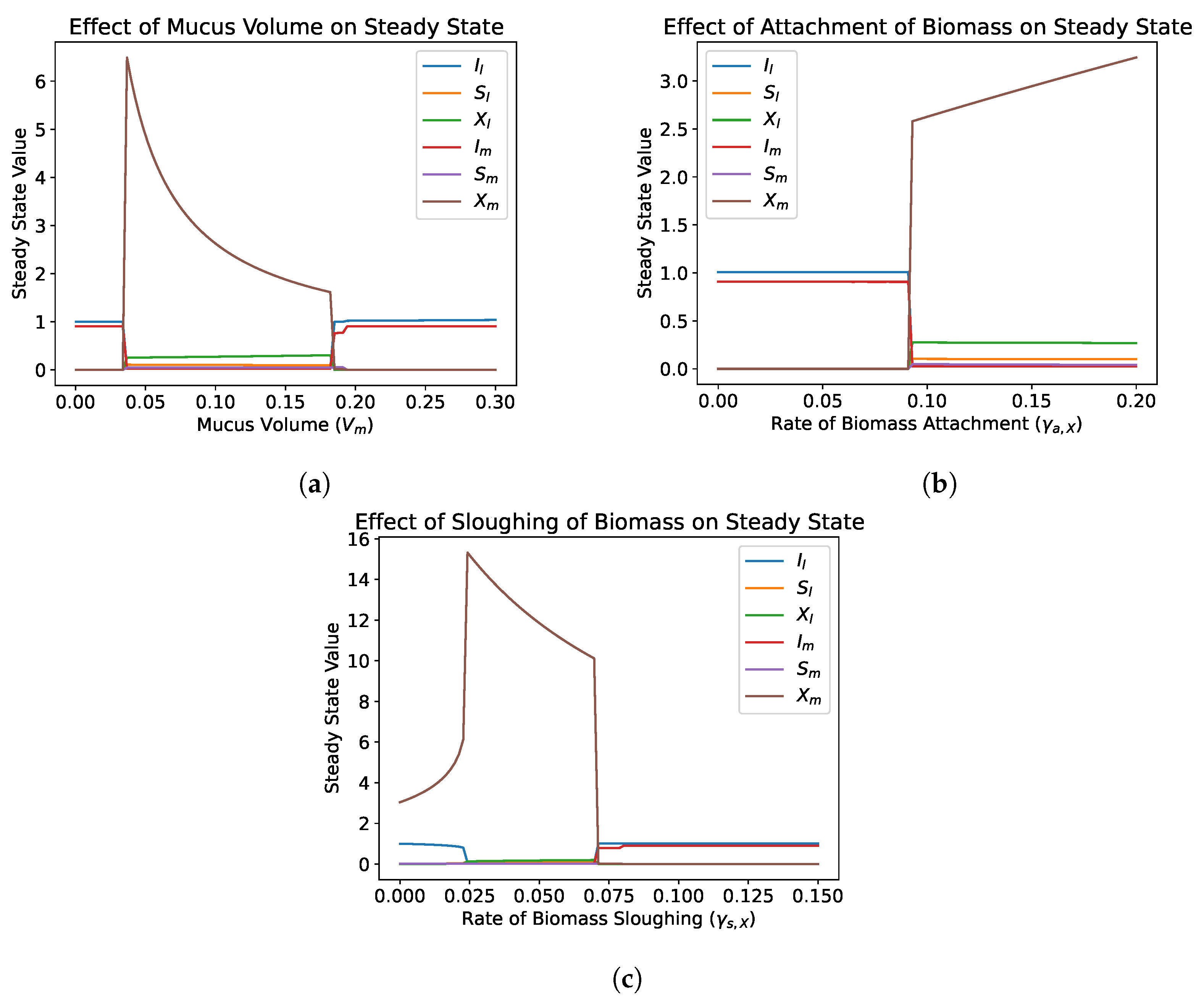
4.2.3. Role of Transfer Parameters

The effect of the exchange of biomass between the two compartments was investigated by varying the attachment (${\gamma }_{a,X}$) and sloughing (${\gamma }_{s,X}$) parameters of X in numerical simulations. The simulations in Figure 6b,c show the effect of varying the exchange rate of X between the lumen and mucus compartments of the reactor. The parameter set used for simulations result in eradication of the species when there is no transfer between compartments, which would correspond to the single compartment model.

In Figure 6b, increasing the attachment rate can shift the system from a washout to the positive equilibrium. Once ${\gamma }_{a,X}$ is large enough for survival, the steady state value of biomass concentration in the mucus $X_m$ increases with ${\gamma }_{a,X}$ but the steady state concentration of biomass in the lumen ($X_l$) decreases at a very low rate.

In Figure 6c, for the sloughing rate ${\gamma }_{s,X}=0$, the system tends to the washout equilibrium. Once the sloughing rate ${\gamma }_{s,X}>0$, the system tends to the positive equilibrium until a critical value of ${\gamma }_{s,X}$, at which washout once again occurs. For ${\gamma }_{s,X}>{\gamma }_{s,C}$, where ${\gamma }_{s,C}$ is the critical value of ${\gamma }_{s,X}$, too much biomass is sloughed from the mucus compartment to the lumen compartment and sloughing can no longer overcome the dilution rate in the lumen.

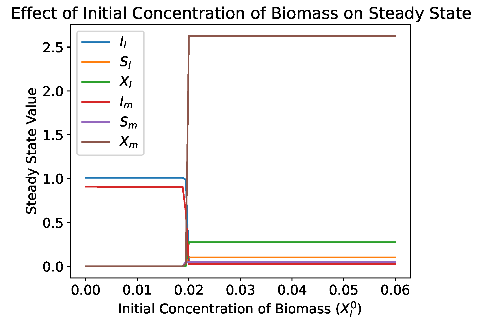
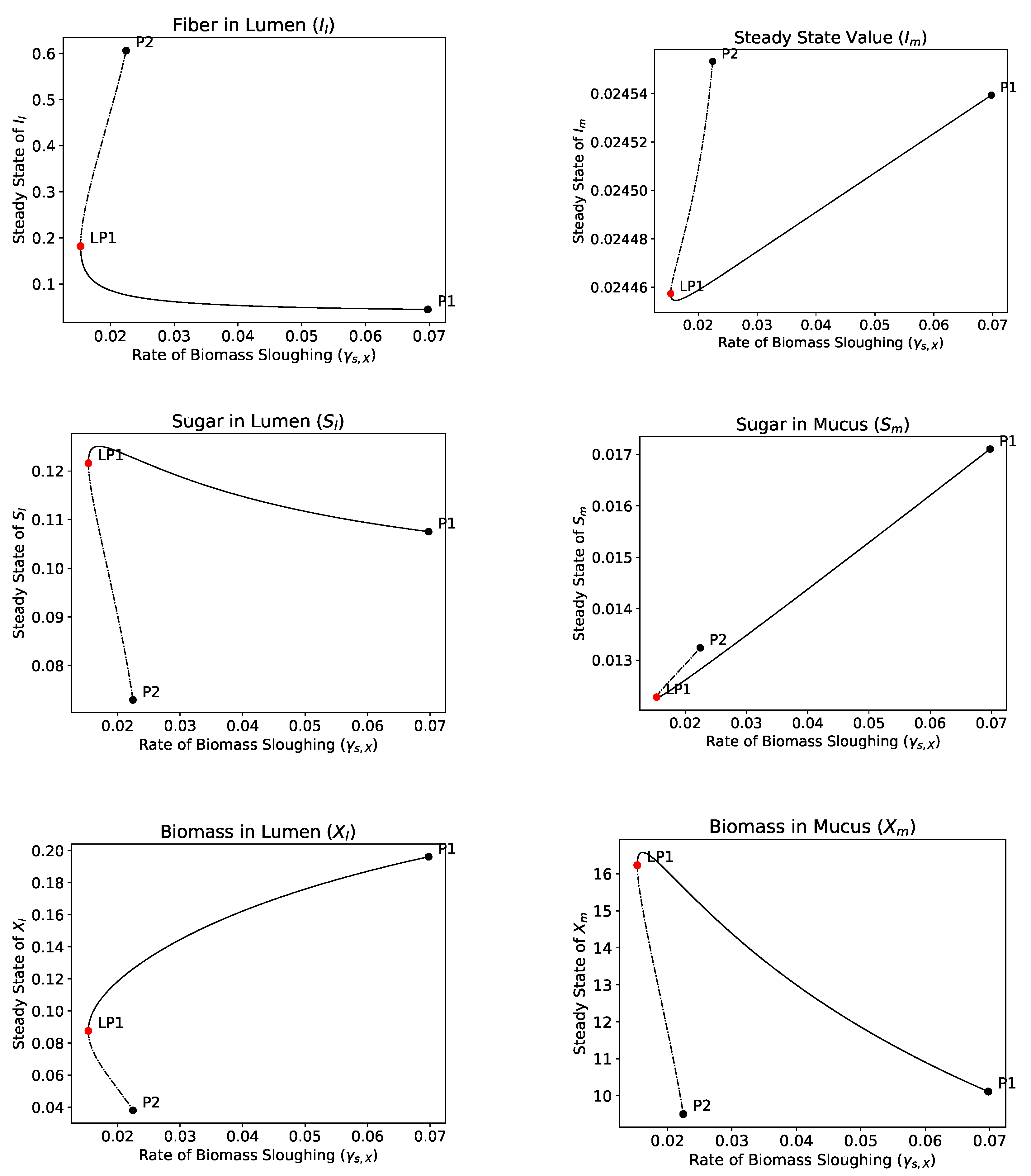
4.2.4. Bifurcation Analysis

As in the single compartment model, the dual compartment model was further investigated using the numerical continuation software in PyDSTool. The figures contained in this section were produced using this software. In Figure 7, the steady states of Equations (4)–(9) are plotted as a function of ${\gamma }_{s,X}$. When ${\gamma }_{s,X}$ is sufficiently large, two positive steady states emerge similarly to Figure 4 showing the emergence of two positive steady states in the single compartment. As in the single compartment, the one of the positive steady states is stable (solid line) and the other positive steady state is unstable (dotted line).

5. Sensitivity Analysis

A variance-based global sensitivity analysis of the model was conducted using the library SALib in Python [27]. The input parameters were sampled using an extension of Sobol’s sequence [28], which is a uniformly-distributed quasi-random sampling method. It is more computationally efficient for the analysis of sensitivity indices than other methods such as random sampling and Latin Hypercube Sampling [29]. This sampling method yields $N=n(2k+2)$ realisations of each simulation, where N is the number of realisations, n is the sample size, and k is the number of model inputs. The estimation of the sensitivity indices were calculated using the Sobol’ analysis, a variance-based global sensitivity analysis method proposed in [30], and extended in [31]. This method is robust to both non-linear and non-monotonic relationships between model inputs and outputs and provides both first-order sensitivity indices and total-order sensitivity indices. The first-order effect indices represent the variance in the output that can be attributed to each input parameter without considering interactions between input parameters. The total effect indices are the sum of the first-order indices and all higher-order indices involving that parameter. The total effect indices represent a parameter’s total contribution to the output variance, combined with all interactions with other parameters. In general, the parameters most influential to model output will have the highest sensitivity indices. We present a sensitivity analysis of the parameter set used in the single compartment model and the parameter set used in the dual compartment model.

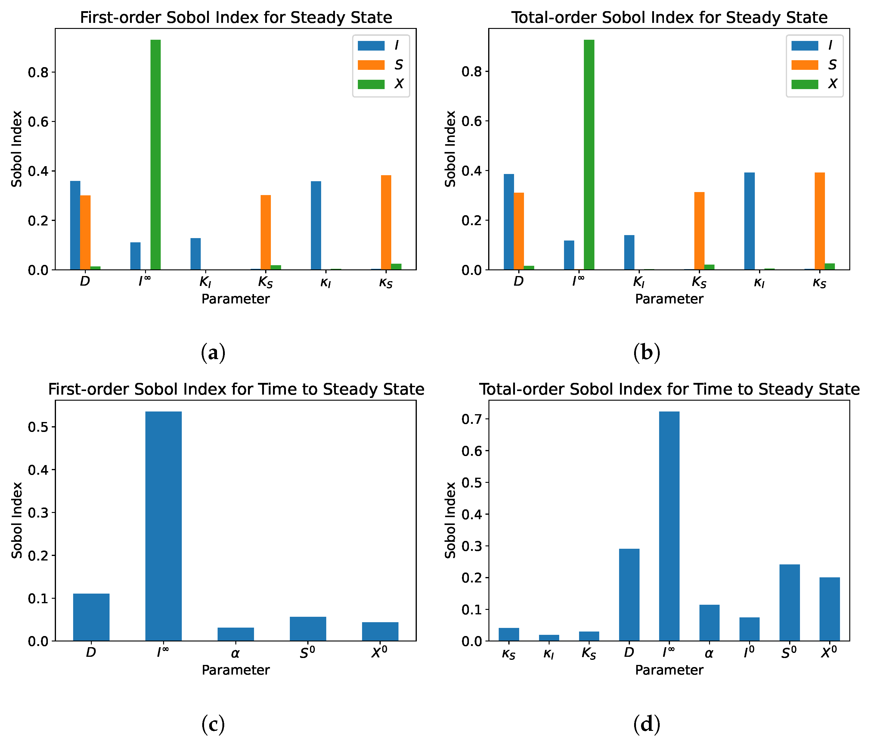
5.1. Single Compartment

In Figure 8 and Figure 9, 1024 samples were used for each set of analyses, which results in 20480 model realisations with the nine parameters considered. The yield coefficients given in Table 1 were held constant through all simulations. The remaining parameters were sampled with a distribution of $\pm 20\%$ the values given in Table 1.

In Figure 8, each simulation concluded with the positive steady state. In Figure 8a,b, the influential parameters for both first- and total-effect indices for steady state values are those that appear in the steady state expressions given in Equations (19) and (20). The first- and total-order sensitivity indices for the time to reach steady state are given in Figure 9c,d. The most influential parameters are those that increase the initial growth rate of the biomass, allowing it to reach a steady state more quickly.

Figure 9a,b show the first-order and total effect sensitivity indices for the steady-state values of I, S, and X. All parameters, except yield coefficients, were sampled in a range of $\pm 20\%$ of the mean values in Table 1, unless otherwise specified. The mean value for initial biomass concentration was set to $X_0=0.035$. With this parameter set and range, particularly the range of $X_0$, it is possible for the system to tend to either the washout equilibrium or the positive equilibrium. As a result, the parameters most influential to the sensitivity indices are those that determine which steady state each simulation will result in, such as the initial concentration of the sugar ($S_0$) and the initial concentration of the biomass ($X_0$), which had no effect in Figure 8a,b. The first- and total-order sensitivity indices are given in Figure 9c,d. As in Figure 9a,b, the most influential parameters are those that determine which equilibrium the system will tend to. If a simulation ends with the system at washout, this occurs at a faster rate than a simulation that results in the positive equilibrium.

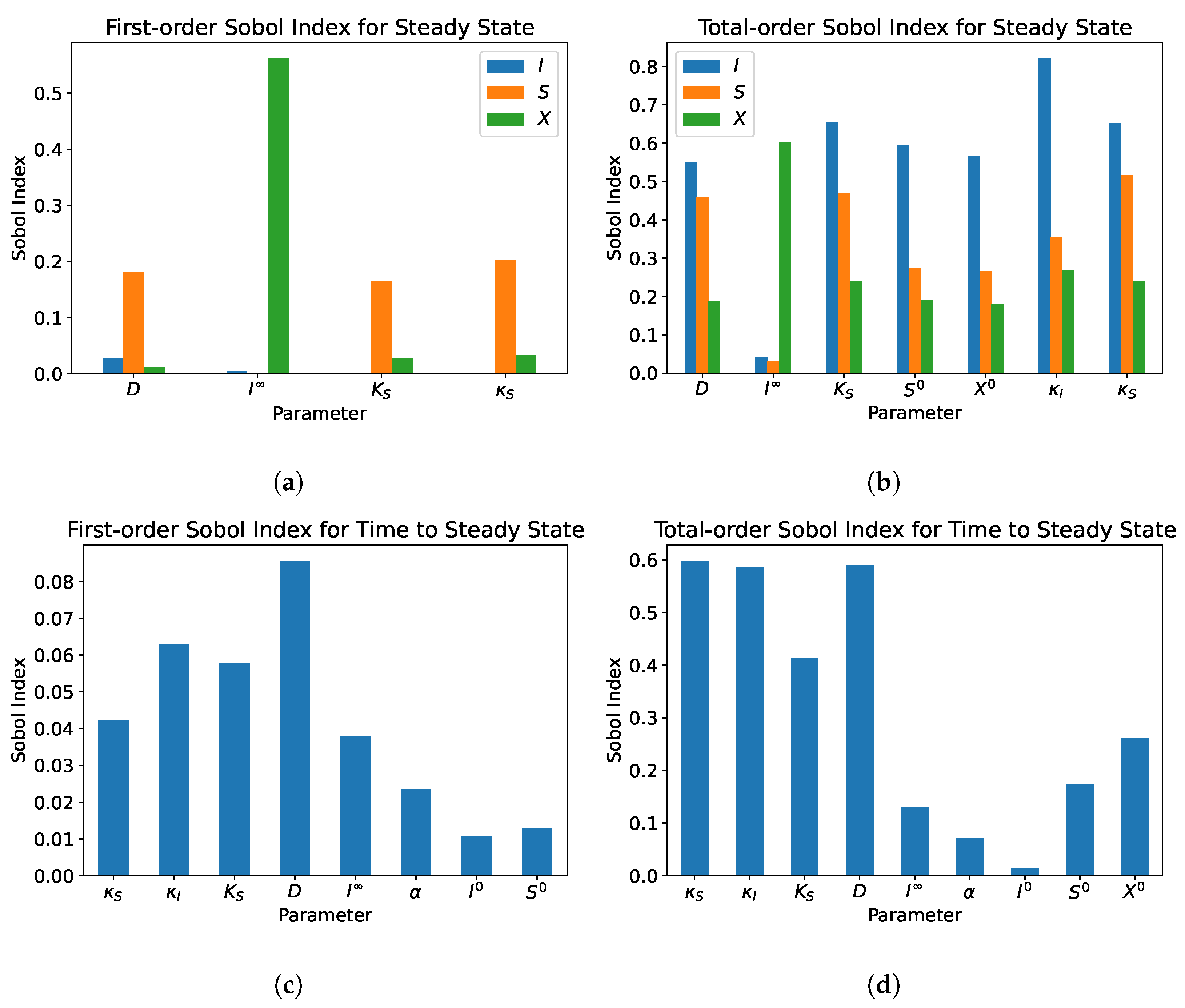
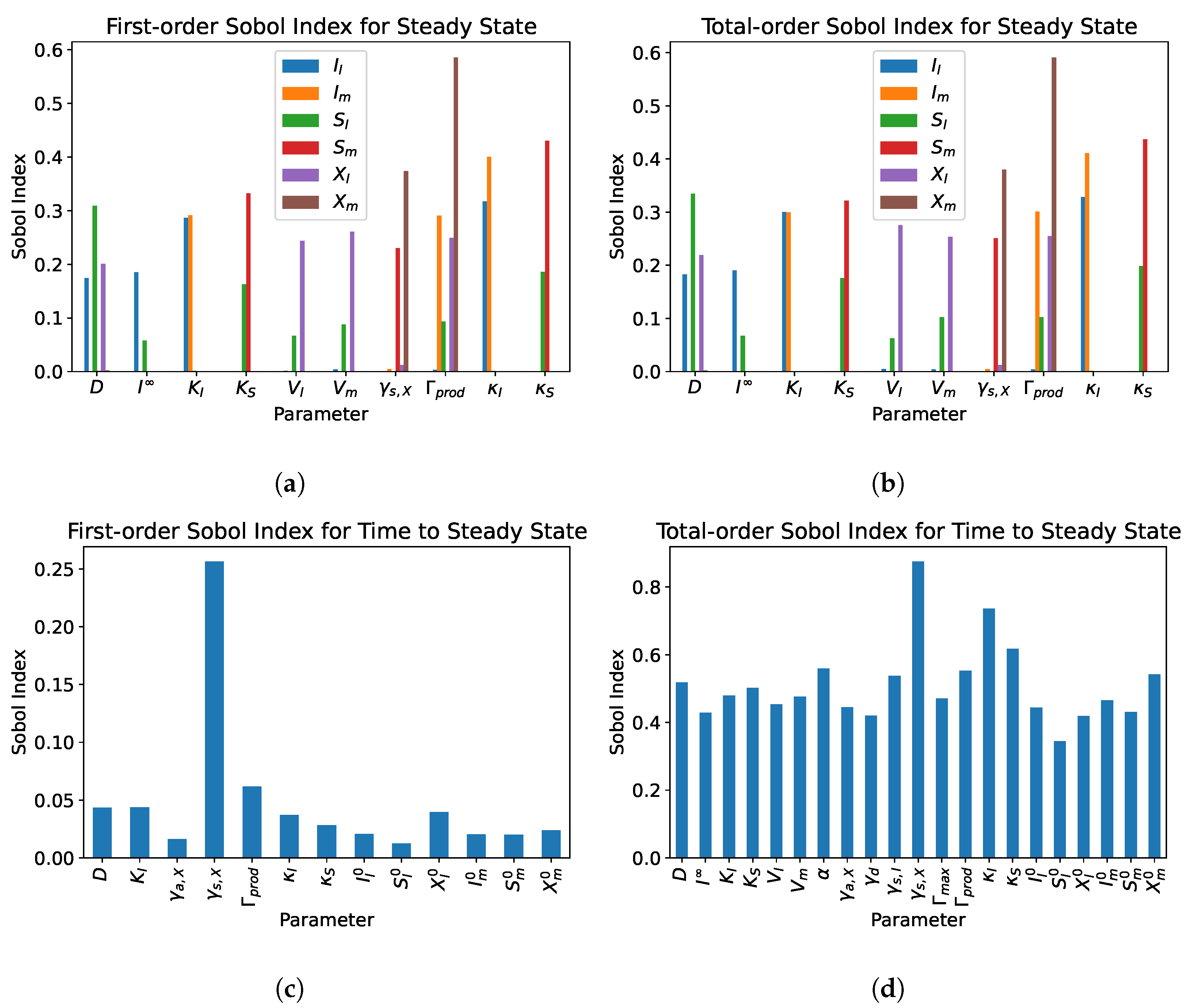
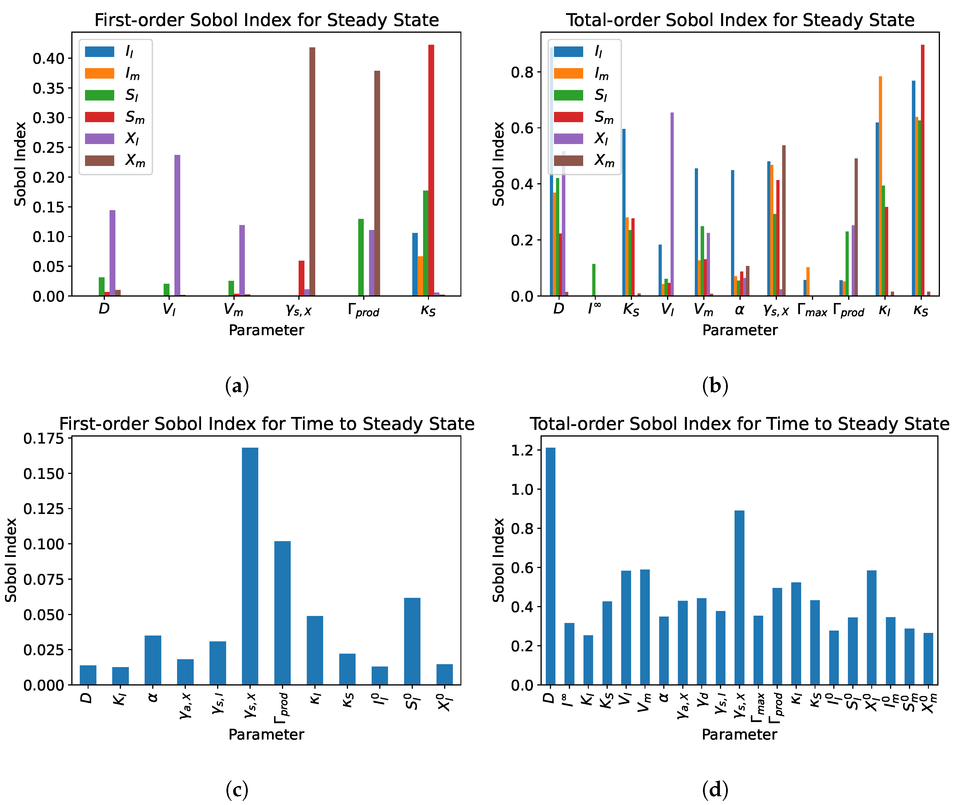
5.2. Dual Compartment Model

In Figure 10 and Figure 11, 1024 samples were used for each set of analyses. This results in 45056 model realisations with the 21 parameters considered. The yield coefficients given in Table 2 were held constant through all simulations. In Figure 10, the remaining parameters were sampled with a distribution of $\pm 20\%$ of the values given in Table 2. In Figure 11, sampling was conducted similarly to Figure 10 but with the parameter range set to $\pm 80\%$ of the mean values given in Table 2 to capture the saddle-node bifurcation (Figure 7). The addition of the mucus compartment results in a narrower range in which the bifurcation can occur.

In Figure 10a,b, each realisation results in the positive steady state, so the most influential parameters are those that affect the final steady state values, as in the single compartment system. For all six variables, the influential parameters include those that effected the corresponding variables in the single compartment system, but also included parameters involved in mucus production (${\mathsf{\Gamma }}_{prod}$) and sloughing of biomass from the mucus to the lumen compartment (${\gamma }_{s,X}$). The parameters that are associated with a compartment tend to influence variables associated with that compartment. For example, the dilution rate (D) and inflow fiber concentration ($I^{\infty }$) only affect luminal variables. When considering the sensitivity of the time to steady state, almost all parameters considered have an affect on the first- and total-sensitivity analysis in Figure 10c,d, with ${\gamma }_{s,X}$ being the most influential.

In Figure 11, each simulation can result in either the washout equilibrium or the positive equilibrium. The parameters that are most impactful on steady state values are those that influence the growth of the biomass (Figure 11a,b). As in Figure 10, the rate of sloughing of biomass from the mucus to the lumen (${\gamma }_{s,X}$) and the rate of mucin production (${\mathsf{\Gamma }}_{prod}$) are the most influential to the steady state values of mucosal biomass $X_m$, and the dilution rate D and the volume of compartments ($V_l$, $V_m$) are most influential to the steady state values of luminal biomass ($X_l$). Unlike the single compartment system, the model outcome is not greatly influenced by the initial concentration of biomass ($X_{l,0}$). The total-order sensitivity indices (Figure 11a) include several additional parameters when compared to the first-order sensitivity indices (Figure 11a). This would suggest that in the dual compartment model, interactions between parameters are greater when the saddle-node bifurcation is captured.

Similarly, in Figure 11c,d, most parameters have some influence, with ${\gamma }_{s,X}$ and ${\mathsf{\Gamma }}_{prod}$ being the most influential. The total-order sensitivity indices in Figure 11d shows that all parameters have influence on the time to steady state, suggesting that there is a high level of interaction between parameters.

6. Discussion

Due to the complexities of interactions within the microbial community in the gut, it can be difficult to attribute outcomes to the specific underlying functions. Several mathematical models of experimental gut reactor systems exist; however, the mechanism of the primary degradation of polysaccharides and the role of the colonic mucus layer have not been extensively considered. In [25], it was found that the recovery of microbiota after antibiotic perturbation depended on the survival and recovery of the microbial group responsible for the primary degradation of carbohydrates. It was also found that antibiotic perturbation that did not result in the immediate eradication of the primary degraders could still result in the extinction of the entire community after antibiotics were no longer present. We considered two mathematical models to investigate the interactions between the commensal microbial community of the colon, dietary fiber and the colonic mucus layer. Our results indicate that these features should be included in gut models for certain applications such as perturbation studies of the human colon.

6.1. Primary Degradation

In the single compartment model (Equations (1)–(3)), a microbial species hydrolyses a polysaccharide into monosaccharides that can then be consumed for growth in a continuous stirred-tank reactor setup. The human gut microbiota rely on the degradation of dietary fiber for energy, and certain microbial groups are responsible for the initial release of energy through hydrolysis [1]. This step has been observed in experimental work to be a rate-limiting step in the digestion of carbohydrates by gut microbiota [32]. Hydrolysis is typically the first step in the multi-stage process of anaerobic digestion, usually consisting of hydrolysis, acidogenesis, acetogenesis and methanogenesis [33]. In the context of reactor control and optimization, similar mathematical models have been considered by [22,34,35]. In [22], both hydrolysis and growth are characterised by monotone increasing functions, such as Monod kinetics. In our model, hydrolysis is defined by the more common Contois kinetics and growth is defined by Monod kinetics. As in [22], we found that the addition of the hydrolysis step results in the unconditional stability of the washout equilibrium. This is in contrast to a system where substrate is readily available for growth and the washout equilibrium is not unconditionally stable. Even when the positive equilibria exists, the washout equilibrium remains stable. As a result, if the initial concentration of the biomass is too low, washout can still occur, even with the existence of a stable equilibrium point. Perturbations to the system that do not result in the eradication of biomass can also unexpectedly lead to washout as observed in the mathematical model in [25] and occasionally in bioreactor experiments [22]. While the total washout of the primary degraders is not a realistic outcome in the human gut, the delay in nutrient consumption caused by hydrolysis may explain the loss of diversity after antibiotic treatment, observed in [36]. In this murine study, while the total abundance of the primary degrader group, Bacteroides, recovered after antibiotic treatment, Bacteroides diversity did not recover. This suggests that certain Bacteroides species are pushed to extinction after antibiotic treatment. To replicate this murine study in a mathematical model, the inclusion of several distinct groups of primary degraders would be necessary.

6.2. Mucus Compartment

The intestinal mucus layer provides a protective habitat for the gut microbiota, providing attachment sites and a source of nutrients. In our second model, we investigated the interplay between primary degraders, dietary fiber, the mucus layer and host-derived mucins. We represented the mucus layer as side compartment attached to the main compartment, as in [13,24]. We found that the bistability exhibited in the single compartment model due to the primary degradation step is preserved even with the addition of the mucus compartment. However, as shown in [24], the addition of a second compartment attached through diffusion results in a system that is less prone to washout when compared to a single compartment system of the same volume. The role of the mucus as a protective environment has also been observed in experimental studies using the M-SHIME reactor [10], where the mucus layer provided a means through which gut microbiota could escape stress. It was also determined in [10] that this protection was not due to the mucins providing extra nutrients. The observations of this experimental gut reactor study support our modelling results and vice versa, and would suggest that the mucus layer, even in its simplest representation, should not be neglected in mathematical and experimental gut reactor models of the gut.

6.3. Importance of Parameters

From the sensitivity analysis of the two models, the most influential parameters affecting the value of the positive steady state are those that directly or indirectly change the concentration of the biomass and thus change the steady state values of sugar and fiber/mucin. When the parameter set can result in each simulation tending towards either the washout equilibrium or the positive equilibrium, the variance in the output is most attributable to which steady state each simulation concludes at. Thus, the parameters that have the most effect are the ones that allow the growth rate at the beginning of the simulation to be sufficiently large for the trajectory to avoid the basin of attraction of the washout equilibrium, such as decreasing the half-saturation constant for growth ($K_S$) or increasing the initial concentration of biomass ($X_0$). Similarly, the variance in time to steady state also depends on whether the initial growth rate of the biomass will be high enough for survival. Time to steady state is much smaller when a simulation goes to the washout equilibrium rather than the positive equilibrium. If the parameter set only allows for the positive equilibrium, then the influential parameters are those that change the steady state concentration of the biomass, such as the supply of substrate to the biomass ($I^{\infty }$) and the amount of time spent in the reactor before the washout (D). In simulations, it was observed that the mucus compartment protects the biomass from washout. When sampling the parameters in the dual compartment model, it was found that the bifurcation is primarily relevant in parameter regimes far from default operating parameters when compared to the single compartment model. These factors are important to consider when designing the composition, timing and optimal doses of therapeutics such as probiotics and prebiotics.

6.4. Implications for Mathematical Models of the Gut

The presented model of primary degradation assumes that primary degraders and complex carbohydrates can be represented as a general group with a single metabolic pathway. To further investigate the relationship between primary degradation, dietary fiber and the mucus layer, as well as their role in dysbiosis and pathologies, multiple representations of primary degraders should be included, with dietary fiber and mucin considered as distinct substrates. To capture disease states associated with low fiber diets and the subsequent thinning of the mucus layer, it is also important to consider the changing volume of mucus and the availability of mucins. Many existing mathematical models of the human colon include subsets of these features and can be extended to consider this relationship as well as the complex bidirectional interaction between host glycan and gut microbes. While the hierarchical nature of the metabolic pathways in the gut allow for the study of simpler models, by considering only the top level of the metabolic processes, cross-feeding and important metabolites, such as short-chain fatty acids, are not considered. We can conclude that studies of dysbiosis and perturbations in the gut may benefit from the inclusion of the hydrolysis pathway and a mucus compartment, but certain applications may also require the incorporation of additional gut features.

7. Conclusions

We have presented a mathematical model of primary degradation of complex carbohydrates in a simplified representation of the human colon. We first considered the hydrolysis of fiber into consumable sugar by a microbial species in a single compartment chemostat reactor representing the lumen of the colon. We further investigated the effect of adding a secondary compartment representing the mucosal environment of the colon as well as endogenously produced mucins as a secondary source of complex carbohydrates.

• In both the single and dual compartment models, the washout equilibrium is unconditionally asymptotically stable. If the biomass concentration is within the basin of attraction of the washout equilibrium, this will result in the washout of the biomass species. This can be due to a perturbation, such as antibiotic treatment, or it can be due to inoculating the reactor with too low of an initial concentration of biomass. This is contrary to the standard single species chemostat model in which the washout equilibrium is unstable when a nontrivial equilibrium exists and survival does not depend on the initial concentration of the biomass.
• The hydrolysis step results in bistability in both the single and dual compartment model. A saddle-node bifurcation appears when the positive equilibrium emerges. This process should not be neglected in mathematical models of the gut and experimental gut reactor systems, particularly in studies of dysbiosis in the gut.
• Numerical simulations show that the addition of the lateral diffusive chamber allows for the survival of microbial species under conditions that would normally result in washout. This depends primarily on the transfer parameters, which can be optimized to maximize the regions that allow for survival. The inclusion of a representation of the mucus layer should be considered in mathematical gut reactor models and experimental gut reactor models.
• Fiber and mucins were considered to be metabolically equivalent in terms of the microbial species that degrade them and the yield and type of monomeric sugars produced. It was also assumed that all primary degraders in the gut can be simplified into a single microbial group that can degrade all complex carbohydrates and reside in both the lumen and mucus environments. In the human gut, there are both generalist and specialist species, each with varying degrees of substrate and environment preferences. For example, abundant generalist species such as Bacteroides thetaiotaomicron are able to shift from dietary polysaccharides to mucus glycans in the absence of fiber, while lower abundance species such as Akkermansia muciniphila can be considered mucus specialists [7]. Additionally, low fiber diets can result in shifts in microbial composition and mucus defects. Future mathematical models should consider the representation of multiple primary degraders, multiple polysaccharides and a dynamic mucus layer to study this interplay.
• From the sensitivity analysis of the single and dual compartment models, different parameters are of importance depending on the desired outcome and should be considered when including therapeutics in simulation design and experiments, e.g., increasing abundance of a target species or preventing the washout of a species.

The mathematical model presented is a simplified representation of the primary degradation in the human. While it is difficult to draw physiological conclusions from this model, it provides a detailed study of a mechanism included in many more sophisticated models of the human colon and can provide justification and direction for future model development.

References

1. Flint, H.J.; Scott, K.P.; Duncan, S.H.; Louis, P.; Forana, E. Microbial degradation of complex carbohydrates in the gut. Gut Microbes 2012, 3, 289–306. [Google Scholar] [CrossRef] [Green Version]
2. Crost, E.H.; Le Gall, G.; Laverde-Gomez, J.A.; Mukhopadhya, I.; Flint, H.J.; Juge, N. Mechanistic insights into the cross-feeding of Ruminococcus gnavus and Ruminococcus bromii on host and dietary carbohydrates. Front. Microbiol. 2018, 9, 2558. [Google Scholar] [CrossRef] [PubMed] [Green Version]
3. Cockburn, D.W.; Koropatkin, N.M. Polysaccharide degradation by the intestinal microbiota and its influence on human health and disease. J. Mol. Biol. 2016, 428, 3230–3252. [Google Scholar] [CrossRef]
4. Li, H.; Limenitakis, J.P.; Fuhrer, T.; Geuking, M.B.; Lawson, M.A.; Wyss, M.; Brugiroux, S.; Keller, I.; Macpherson, J.A.; Rupp, S.; et al. The outer mucus layer hosts a distinct intestinal microbial niche. Nat. Commun. 2015, 6, 8292. [Google Scholar] [CrossRef] [Green Version]
5. Paone, P.; Cani, P.D. Mucus barrier, mucins and gut microbiota: The expected slimy partners? Gut 2020, 69, 2232–2243. [Google Scholar] [CrossRef] [PubMed]
6. McDonald, J.A.; Schroeter, K.; Fuentes, S.; Heikamp-deJong, I.; Khursigara, C.M.; de Vos, W.M.; Allen-Vercoe, E. Evaluation of microbial community reproducibility, stability and composition in a human distal gut chemostat model. J. Microbiol. Methods 2013, 95, 167–174. [Google Scholar] [CrossRef]
7. Sauvaitre, T.; Etienne-Mesmin, L.; Sivignon, A.; Mosoni, P.; Courtin, C.M.; Van de Wiele, T.; Blanquet-Diot, S. Tripartite relationship between gut microbiota, intestinal mucus and dietary fibers: Towards preventive strategies against enteric infections. FEMS Microbiol. Rev. 2021, 45, fuaa052. [Google Scholar]
8. Peterson, C.T.; Sharma, V.; Elmén, L.; Peterson, S.N. Immune homeostasis, dysbiosis and therapeutic modulation of the gut microbiota. Clin. Ex. Immunol. 2015, 179, 363–377. [Google Scholar] [CrossRef] [Green Version]
9. Roupar, D.; Berni, P.; Martins, J.T.; Caetano, A.C.; Teixeira, J.A.; Nobre, C. Bioengineering approaches to simulate human colon microbiome ecosystem. Trends Food Sci. Technol. 2021, 112, 808–822. [Google Scholar] [CrossRef]
10. De Weirdt, R.; Coenen, E.; Vlaeminck, B.; Fievez, V.; Van den Abbeele, P.; Van de Wiele, T. A simulated mucus layer protects Lactobacillus reuteri from the inhibitory effects of linoleic acid. Benef. Microbes 2013, 4, 299–312. [Google Scholar] [CrossRef] [PubMed]
11. Nissen, L.; Casciano, F.; Gianotti, A. Intestinal fermentation in vitro models to study food-induced gut microbiota shift: An updated review. FEMS Microbiol. Lett. 2020, 367, fnaa097. [Google Scholar] [CrossRef] [PubMed]
12. Allen-Vercoe, E. Bringing the gut microbiota into focus through microbial culture: Recent progress and future perspective. Curr. Opin. Microbiol. 2013, 16.5, 625–629. [Google Scholar] [CrossRef] [PubMed] [Green Version]
13. Muñoz-Tamayo, R.; Laroche, B.; Walter, E.; Doré, J.; Leclerc, M. Mathematical modelling of carbohydrate degradation by human colonic microbiota. J. Theor. Biol. 2010, 266, 189–201. [Google Scholar] [CrossRef] [PubMed]
14. Batstone, D.J.; Keller, J.; Angelidaki, I.; Kalyuzhnyi, S.V.; Pavlostathis, S.G.; Rozzi, A.; Sanders, W.T.M.; Siegrist, H.A.; Vavilin, V.A. The IWA anaerobic digestion model no 1 (ADM1). Water Sci. Technol. 2002, 45, 65–73. [Google Scholar] [CrossRef] [PubMed]
15. Motelica-Wagenaar, A.M.; Nauta, A.; van den Heuvel, E.G.; Kleerebezem, R. Flux analysis of the human proximal colon using anaerobic digestion model 1. Anaerobe 2014, 28, 137–148. [Google Scholar] [CrossRef]
16. Kettle, H.; Louis, P.; Holtrop, G.; Duncan, S.H.; Flint, H.J. Modelling the emergent dynamics and major metabolites of the human colonic microbiota. Environ. Microbiol. 2015, 17, 1615–1630. [Google Scholar] [CrossRef] [Green Version]
17. Moorthy, A.S.; Brooks, S.P.; Kalmokoff, M.; Eberl, H.J. A spatially continuous model of carbohydrates digestion and transport processes in the colon. PLoS ONE 2015, 10, e0145309. [Google Scholar] [CrossRef] [Green Version]
18. Kettle, H.; Holtrop, G.; Louis, P.; Flint, H.J. micropop: Modelling microbial populations and communities in R. MEE 2018, 9, 399–409. [Google Scholar] [CrossRef] [Green Version]
19. Moorthy, A.S.; Eberl, H.J. compuGUT: An in silico platform for simulating intestinal fermentation. SoftwareX 2017, 6, 237–242. [Google Scholar] [CrossRef]
20. Cremer, J.; Arnoldini, M.; Hwa, T. Effect of water flow and chemical environment on microbiota growth and composition in the human colon. Proc. Natl. Acad. Sci. USA 2017, 114, 6438–6443. [Google Scholar] [CrossRef] [Green Version]
21. Labarthe, S.; Polizzi, B.; Phan, T.; Goudon, T.; Ribot, M.; Laroche, B. A mathematical model to investigate the key drivers of the biogeography of the colon microbiota. J. Theor. Biol. 2019, 462, 552–581. [Google Scholar] [CrossRef] [PubMed] [Green Version]
22. Tang, B.; Wolkowicz, G. Mathematical models of microbial growth and competition in the chemostat regulated by cell-bound extracellular enzymes. J. Math. Biol. 1992, 31, 1–23. [Google Scholar] [CrossRef]
23. Smith, H.L.; Waltman, P. The Theory of the Chemostat: Dynamics of Microbial Competition, 1st ed.; Cambridge University Press: Cambridge, UK, 1995; pp. 1–14. [Google Scholar]
24. Crespo, M.; Rapaport, A. Analysis and Optimization of the Chemostat Model with a Lateral Diffusive Compartment. J. Optim. Theory Appl. 2020, 185, 597–621. [Google Scholar] [CrossRef]
25. Jegatheesan, T.; Eberl, H.J. Modelling the Effects of Antibiotics on Gut Flora Using a Nonlinear Compartment Model with Uncertain Parameters. ICCS 2020, 12137, 399–412. [Google Scholar]
26. Walter, W. Ordinary Differential Equations, 1st ed.; Springer Science & Business Media: New York, NY, USA, 1998; pp. 148–157. [Google Scholar]
27. Herman, J.; Usher, W. SALib: An open-source Python library for Sensitivity Analysis. J. Open Source Softw. 2017, 2, 97. [Google Scholar] [CrossRef]
28. Saltelli, A. Making best use of model evaluations to compute sensitivity indices. Comput. Phys. Commun. 2002, 145, 280–297. [Google Scholar] [CrossRef]
29. Saltelli, A.; Annoni, P. How to avoid a perfunctory sensitivity analysis. Environ. Model. Softw. 2010, 25, 1508–1517. [Google Scholar] [CrossRef]
30. Sobol’, I.M. Global sensitivity indices for nonlinear mathematical models and their Monte Carlo estimates. Math. Comput. Simul. 2001, 55, 271–280. [Google Scholar] [CrossRef]
31. Saltelli, A.; Annoni, P.; Azzini, I.; Campolongo, F.; Ratto, M.; Tarantola, S. Variance based sensitivity analysis of model output. Design and estimator for the total sensitivity index. Comput. Phys. Commun. 2010, 181, 259–270. [Google Scholar] [CrossRef]
32. Oliphant, K.; Allen-Vercoe, E. Macronutrient metabolism by the human gut microbiome: Major fermentation by-products and their impact on host health. Microbiome 2019, 7, 1–15. [Google Scholar] [CrossRef]
33. Wade, M.J. Not Just Numbers: Mathematical Modelling and Its Contribution to Anaerobic Digestion Processes. Processes 2020, 8, 888. [Google Scholar] [CrossRef]
34. Fekih-Salem, R.; Abdellatif, N.; Sari, T.; Harmand, J. On a three step model of anaerobic digestion including the hydrolysis of particulate matter. IFAC Proc. Vol. 2012, 45, 671–676. [Google Scholar] [CrossRef] [Green Version]
35. Hanaki, M.; Harmand, J.; Mghazli, Z.; Sari, T.; Rapaport, A.; Ugalde, P. Mathematical study of a two-stage anaerobic model when the hydrolysis is the limiting step. Processes 2021, 9, 2050. [Google Scholar] [CrossRef]
36. Ng, K.M.; Aranda-Díaz, A.; Tropini, C.; Frankel, M.R.; Treuren, W.V.; O’Loughlin, C.T.; Merrill, B.D.; Yu, F.B.; Pruss, K.M.; Oliveira, R.A.; et al. Recovery of the Gut Microbiota after Antibiotics Depends on Host Diet, Community Context and Environmental Resevoirs. Cell Host Microbe 2019, 25, 650–665. [Google Scholar] [CrossRef] [PubMed]
Figure 1. The reactor representation of the single compartment model. The compartment is fully mixed. There is inflow of fiber ( I ) and outflow of fiber (I), sugar (S) and biomass (X).
Processes 11 00370 g001
Figure 2. The reactor representation of the dual compartment model. Both compartments are fully mixed. For the lumen compartment, there is inflow of fiber ( I ) and outflow of fiber ( I l ), sugar ( S l ) and biomass ( X l ). There is transport of sugar ( S i ) and biomass ( X i ) between the lumen and mucus compartments, where i { l , m } . There is no transport of fiber ( I l ) between compartments. Transport of mucin ( I m ) is unidirectional from the mucus to the lumen.
Processes 11 00370 g002
Figure 3. Steady state values of fiber (I), sugar (S) and biomass concentration (X) as a function of (a) dilution rate (D), (b) inflow fiber concentration ( I ), and (c) initial biomass concentration ( X 0 ).
Processes 11 00370 g003
Figure 4. Bifurcation diagrams showing the steady states of (a) fiber ( I 1 , 2 * ), (b) sugar ( S * ), and (c) biomass ( X 1 , 2 * ) as a function of inflow fiber concentration ( I ). The solid and dashed lines indicate stable and unstable steady states, respectively. P1 and P2 refer to the start and end points of the continuation. LP1 is the limit point.
Processes 11 00370 g004
Figure 5. The effect of initial concentration of lumen biomass concentration ( X l , 0 ) on steady state concentration values in the dual compartment model.
Processes 11 00370 g005
Figure 6. (a) Steady state concentration values of the dual compartment model as a function of mucus volume ( V m ). The total reactor volume was held constant ( V m + V l = 1.0 ). (b) Steady state values of the dual compartment model as a function of the rate of biomass attachment from the lumen to mucus ( γ a , X ). (c) Steady state values of the dual compartment model as a function of the rate of biomass sloughing from the mucus to lumen ( γ s , X ).
Processes 11 00370 g006
Figure 7. Steady state values of dual compartment model (Equations (4)–(9)) plotted as a function of the rate of sloughing of biomass from the mucus to lumen ( γ s , X ). The solid and dashed lines indicate stable and unstable steady states, respectively. P1 and P2 refer to the start and end points of the continuation. LP1 is the limit point.
Processes 11 00370 g007
Figure 8. (a) First-order and (b) total effect sensitivity indices of steady-state values of fiber I, sugar S and biomass X. (c) First-order and (d) total effect sensitivity indices of time to steady state values of fiber I, sugar S and biomass X for a parameter set that tends to the positive steady state. Sampling was conducted with a variance of 20 % on input parameters, excluding yield coefficients. Mean values were taken from Table 1.
Processes 11 00370 g008
Figure 9. (a) First-order and (b) total effect sensitivity indices of time to steady state values of fiber I, sugar S and biomass X. (c) First-order and (d) total effect sensitivity indices of time to steady state values of fiber I, sugar S and biomass X. Sampling was conducted with a variance of 20 % on input parameters, excluding yield coefficients. Mean values were taken from Table 1, excluding initial biomass concentration, which was set to X 0 = 0.035 . This parameter set captures the saddle-node bifurcation (Figure 4).
Processes 11 00370 g009
Figure 10. (a) First-order and (b) total effect sensitivity indices of steady-state values of fiber I l , mucin I m , luminal sugar S l , mucosal sugar S m , luminal biomass X l and mucosal biomass X m . Parameters with sensitivity indices below 0.1 for all variables were omitted for (a,b). (c) First-order and (d) total effect sensitivity indices of time to steady state of fiber I l , mucin I m , luminal sugar S l , mucosal sugar S m , luminal biomass X l and mucosal biomass X m . Parameters with sensitivity indices below 0.01 were omitted for (c,d). Sampling was conducted with a variance of 20 % on input parameters, excluding yield coefficients. Mean values were taken from Table 2.
Processes 11 00370 g010
Figure 11. (a) First-order and (b) total effect sensitivity indices of steady-state values of fiber I l , mucin I m , luminal sugar S l , mucosal sugar S m , luminal biomass X l and mucosal biomass X m . Parameters with sensitivity indices below 0.1 for all variables were omitted for (a,b). (c) First-order and (d) total effect sensitivity indices of time to steady state of fiber I l , mucin I m , luminal sugar S l , mucosal sugar S m , luminal biomass X l and mucosal biomass X m . Parameters with sensitivity indices below 0.01 were omitted for (c,d). Sampling was conducted with a variance of 80 % on input parameters to capture the saddle-node bifurcation (Figure 7), excluding yield coefficients. Mean values were taken from Table 2.
Processes 11 00370 g011