
Numerical Simulations of Gasification of Low-Grade Coal and Lignocellulosic Biomasses in Two-Stage Multi-Opposite Burner Gasifier

 ,
,
Abstract
:1. Introduction
2. Numerical Method
2.1. CFD Model Development
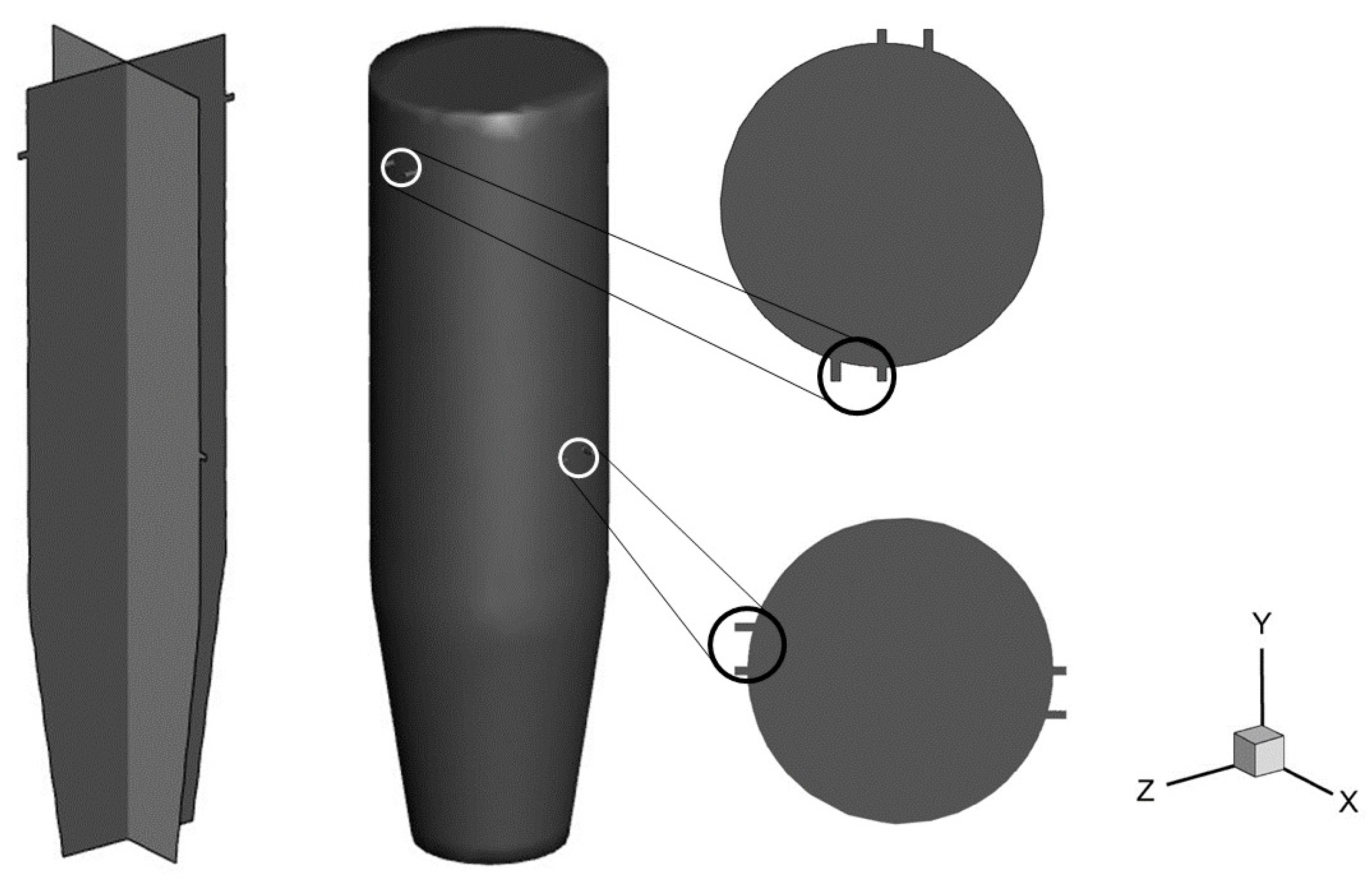
2.2. Computational Domain
2.3. Governing Equations and Assumptions
2.4. Chemical Reactions
2.5. Feedstock Composition, Operating Parameters, and Performance Indicators
2.6. Conditions at Boundary Zones and Solution Strategies
3. Results and Discussion
3.1. Validation of Reaction Schemes
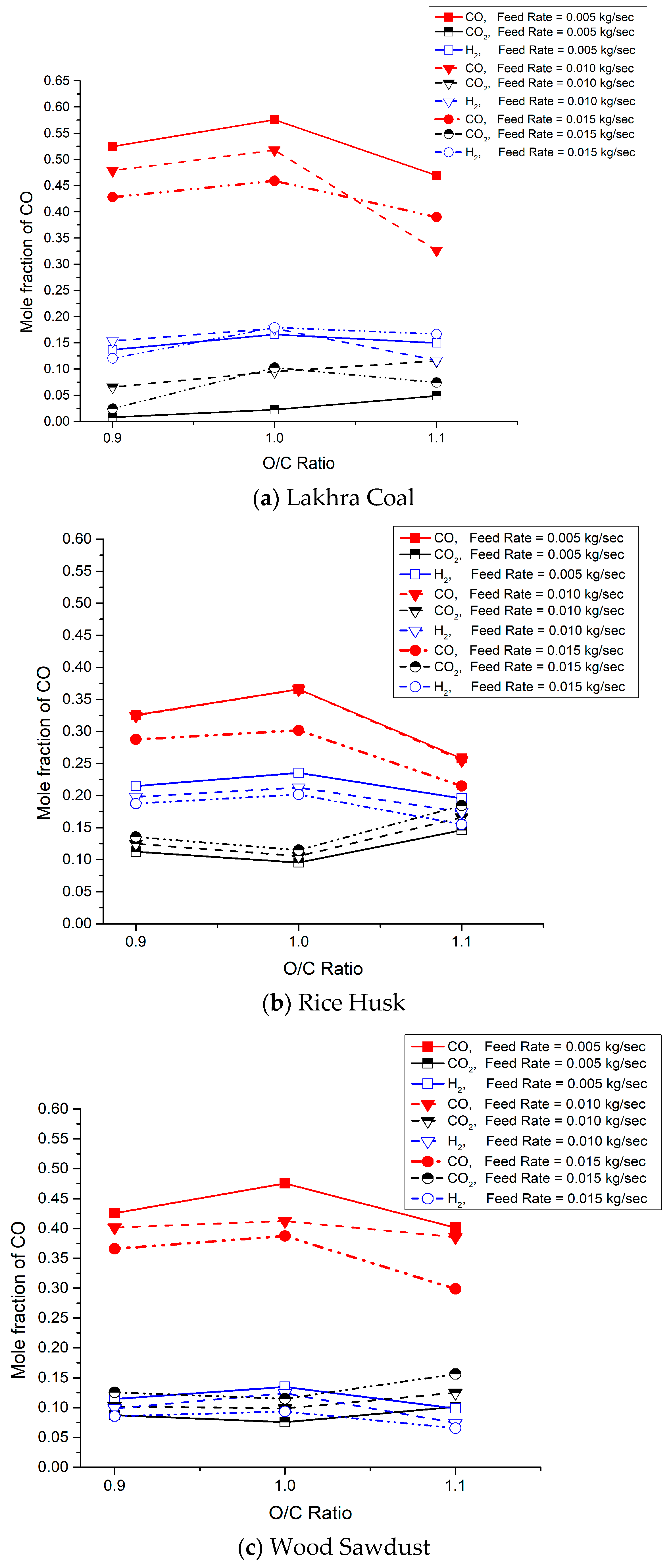
3.2. Syngas Composition
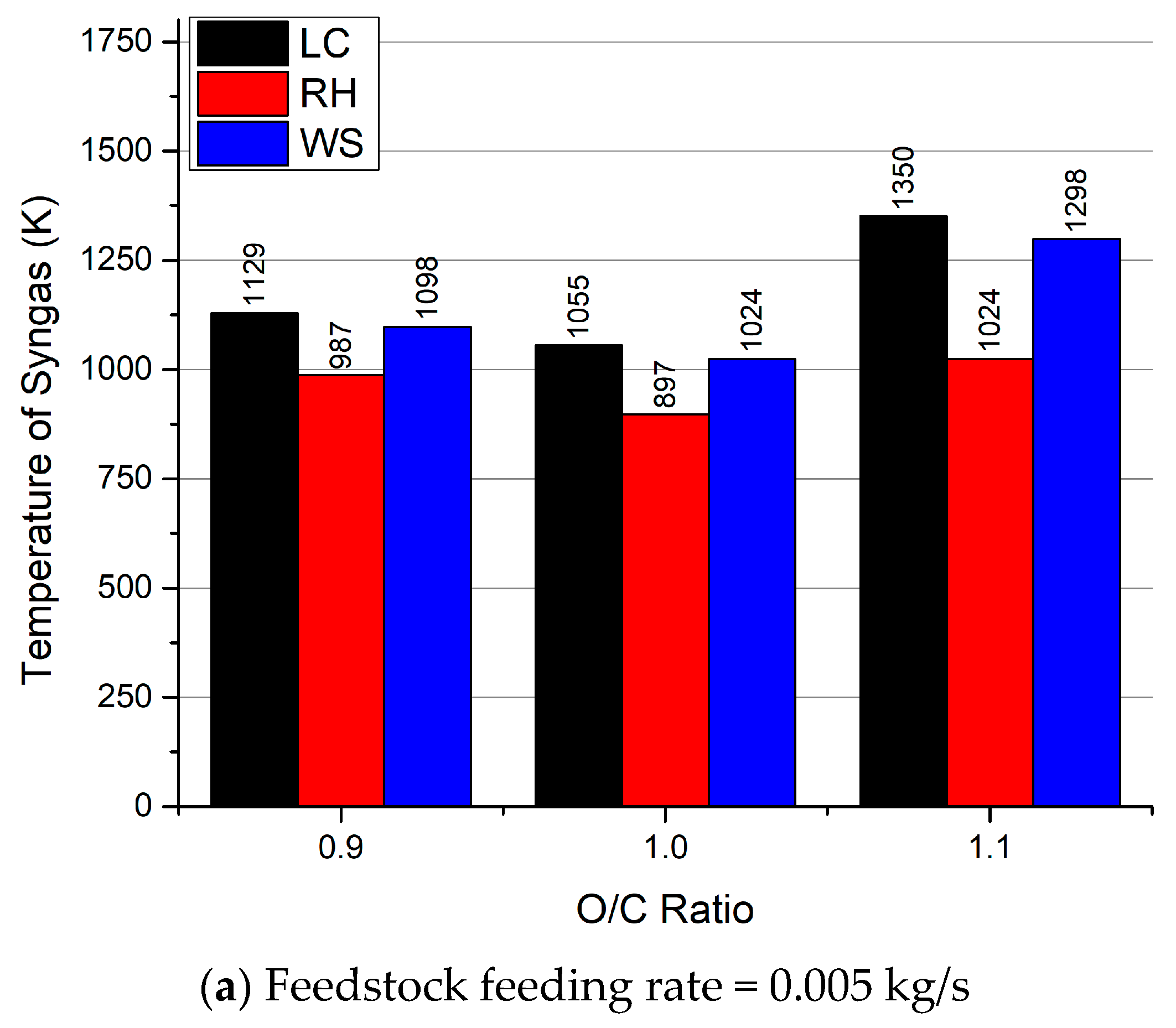
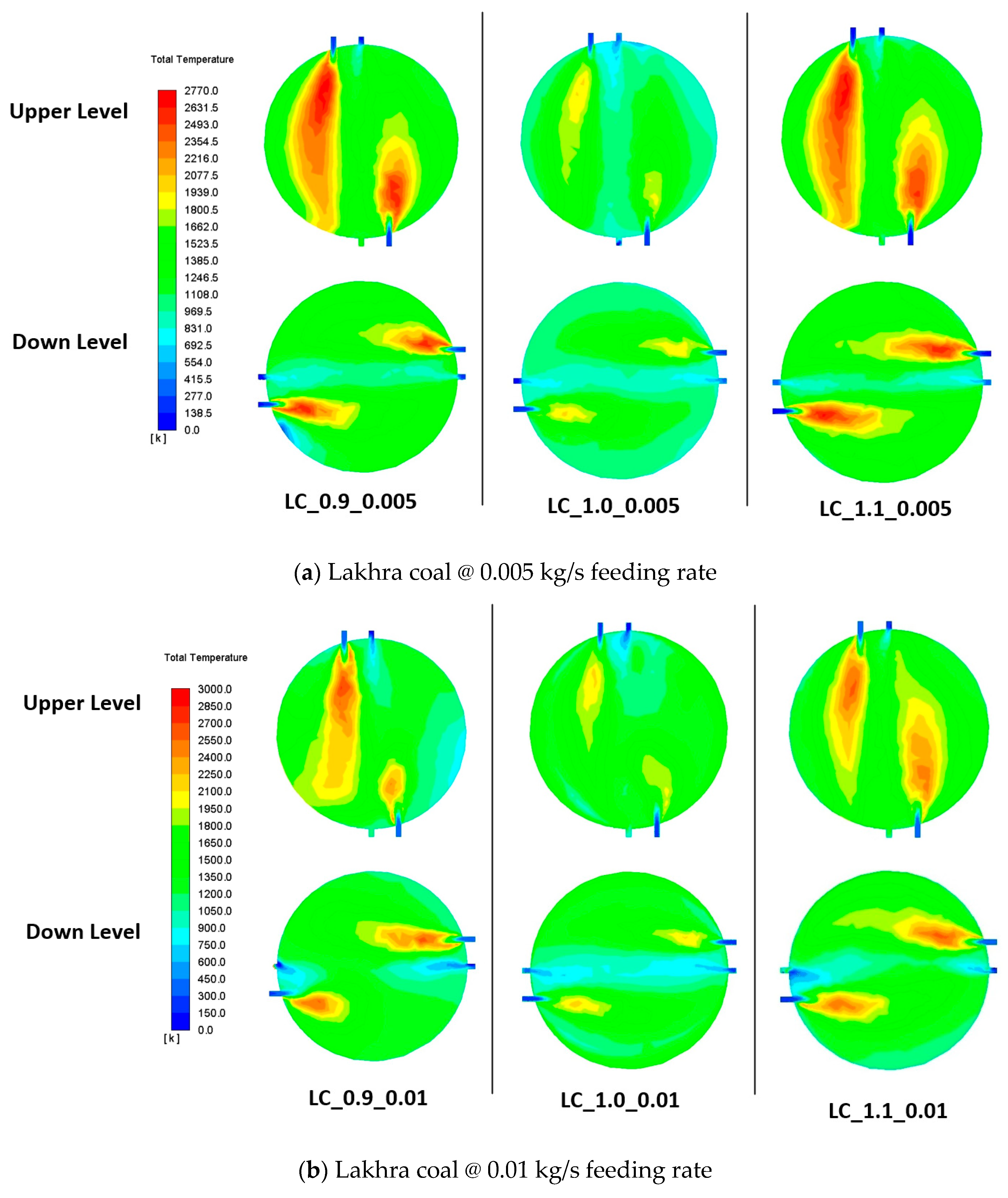
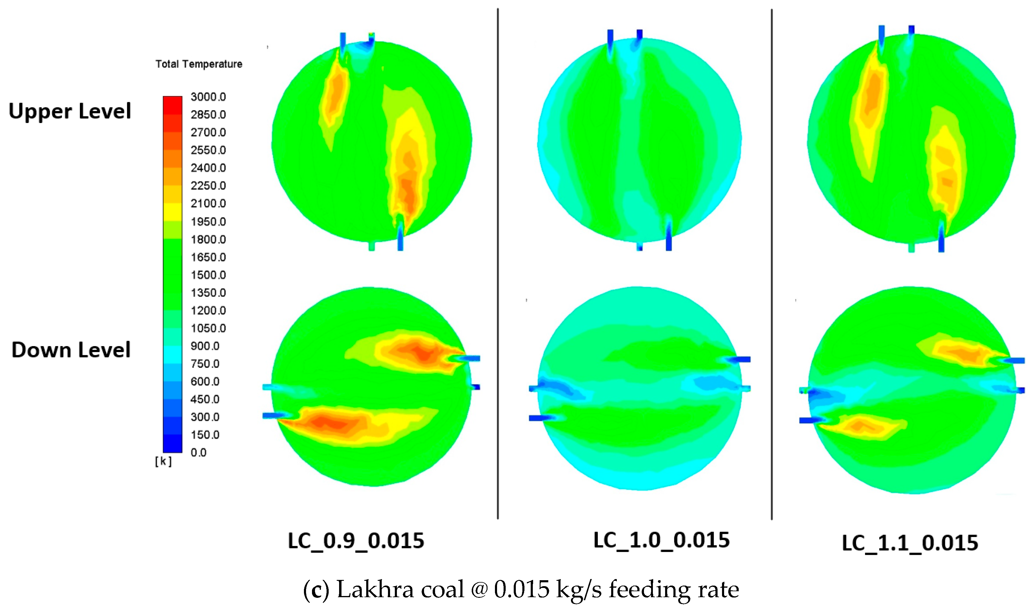
3.3. Temperature of Gasification
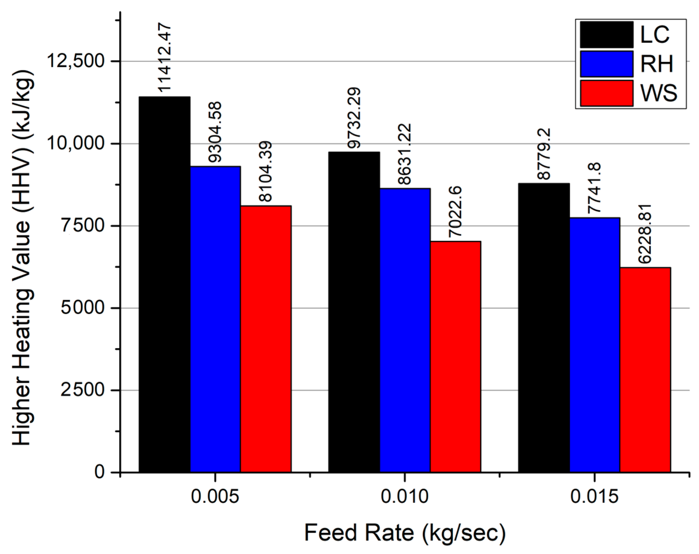
3.4. Quality of Produced Syngas
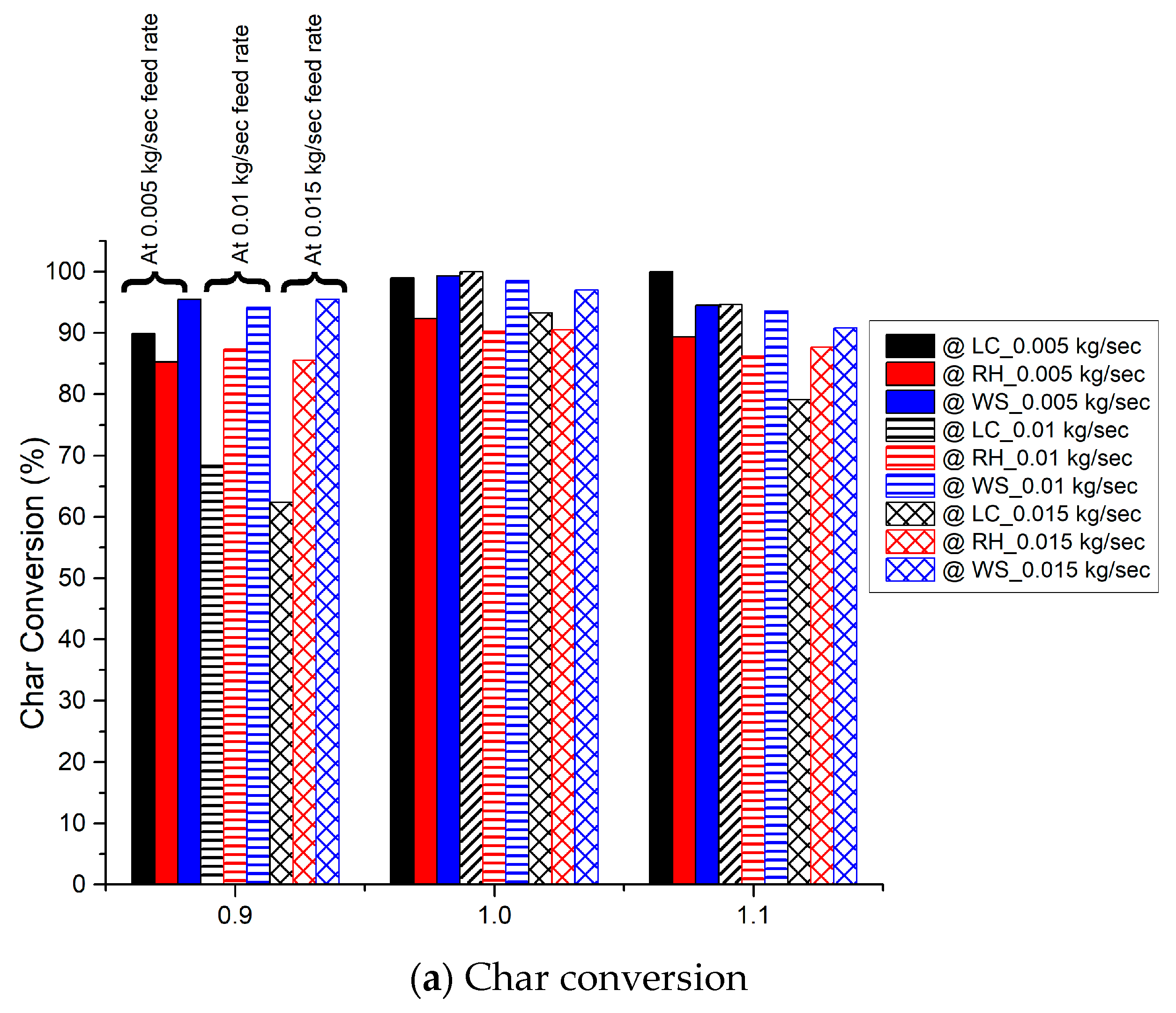
3.5. Conversion of Char and Volatiles
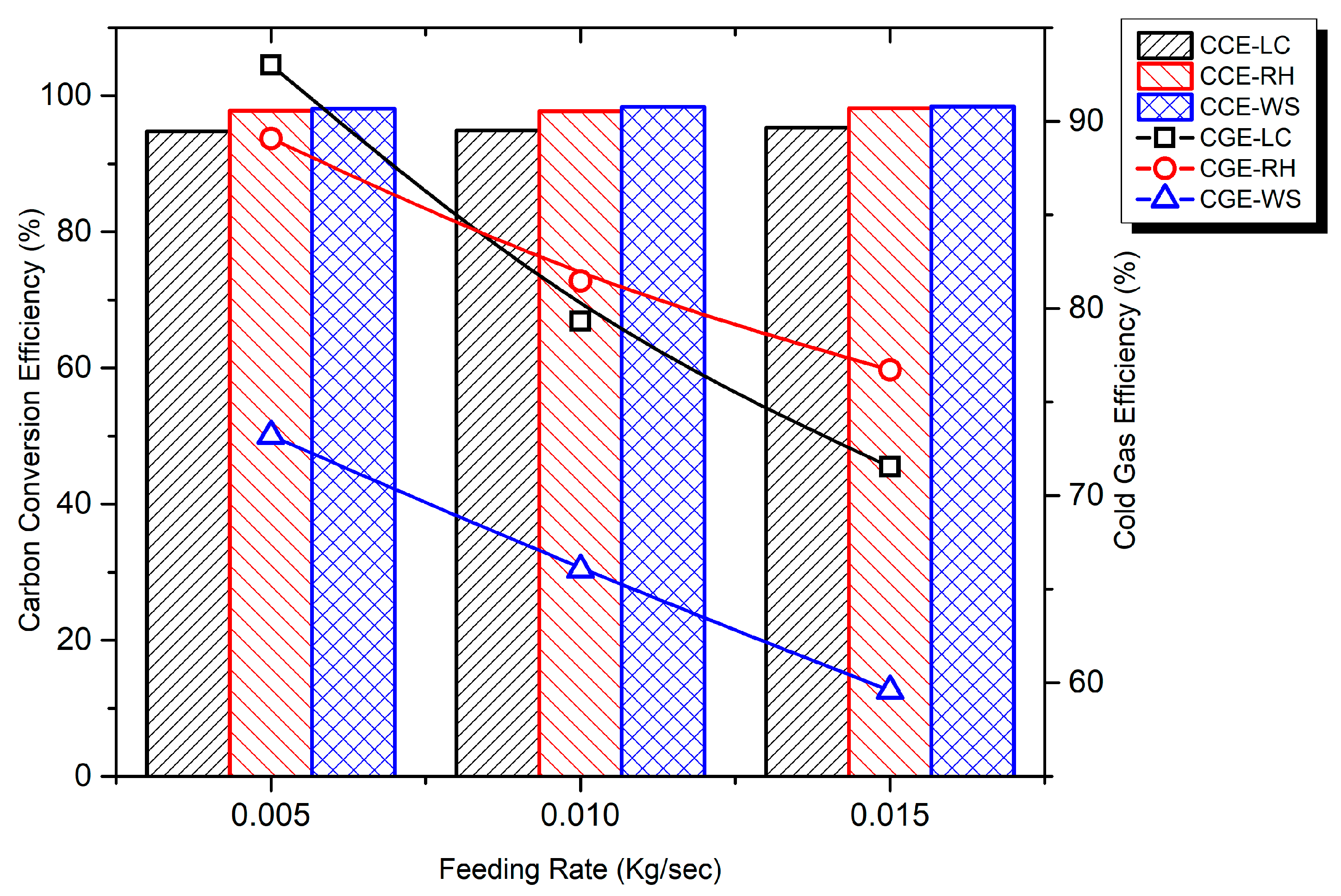
3.6. Conversion Efficiencies
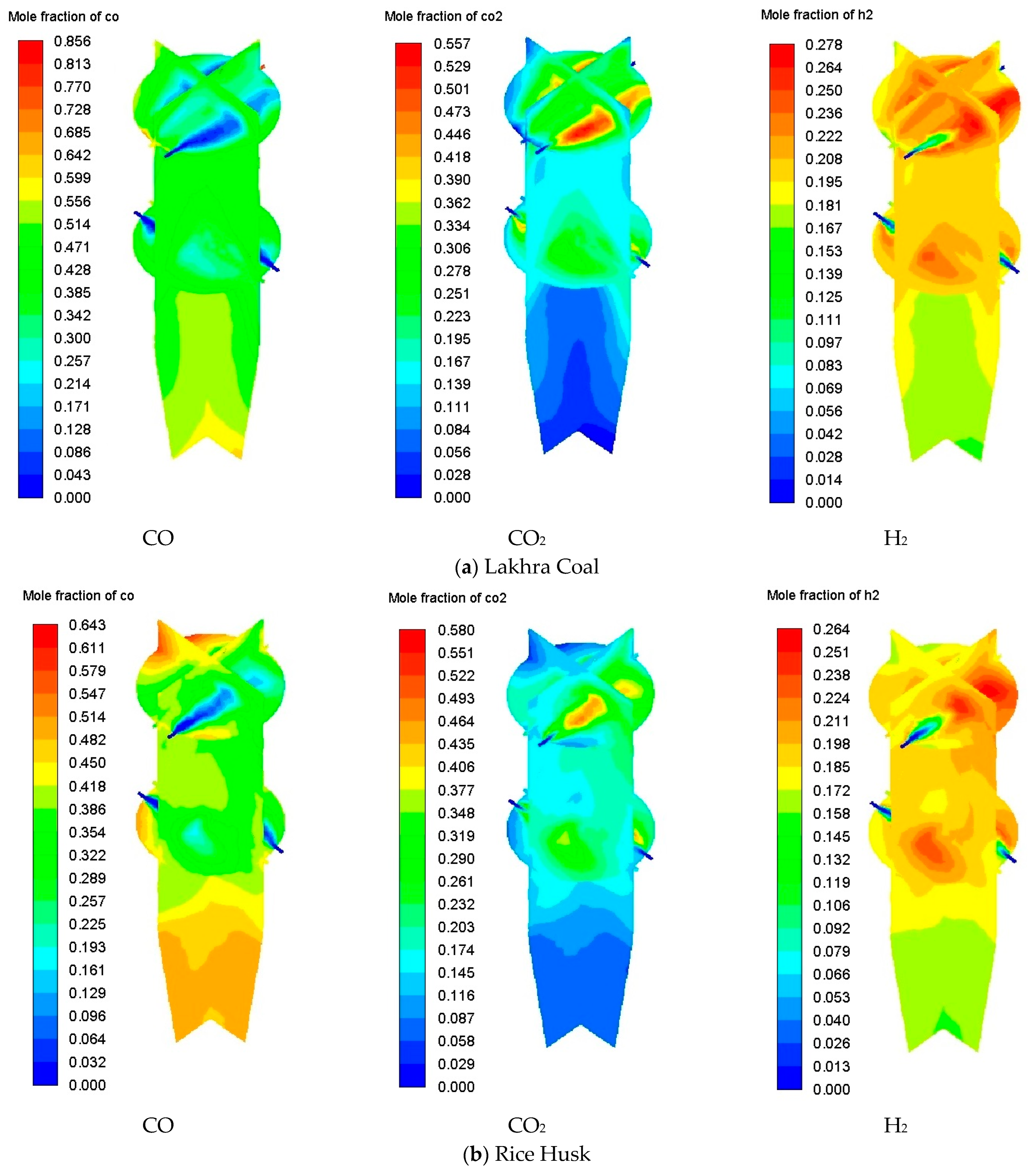
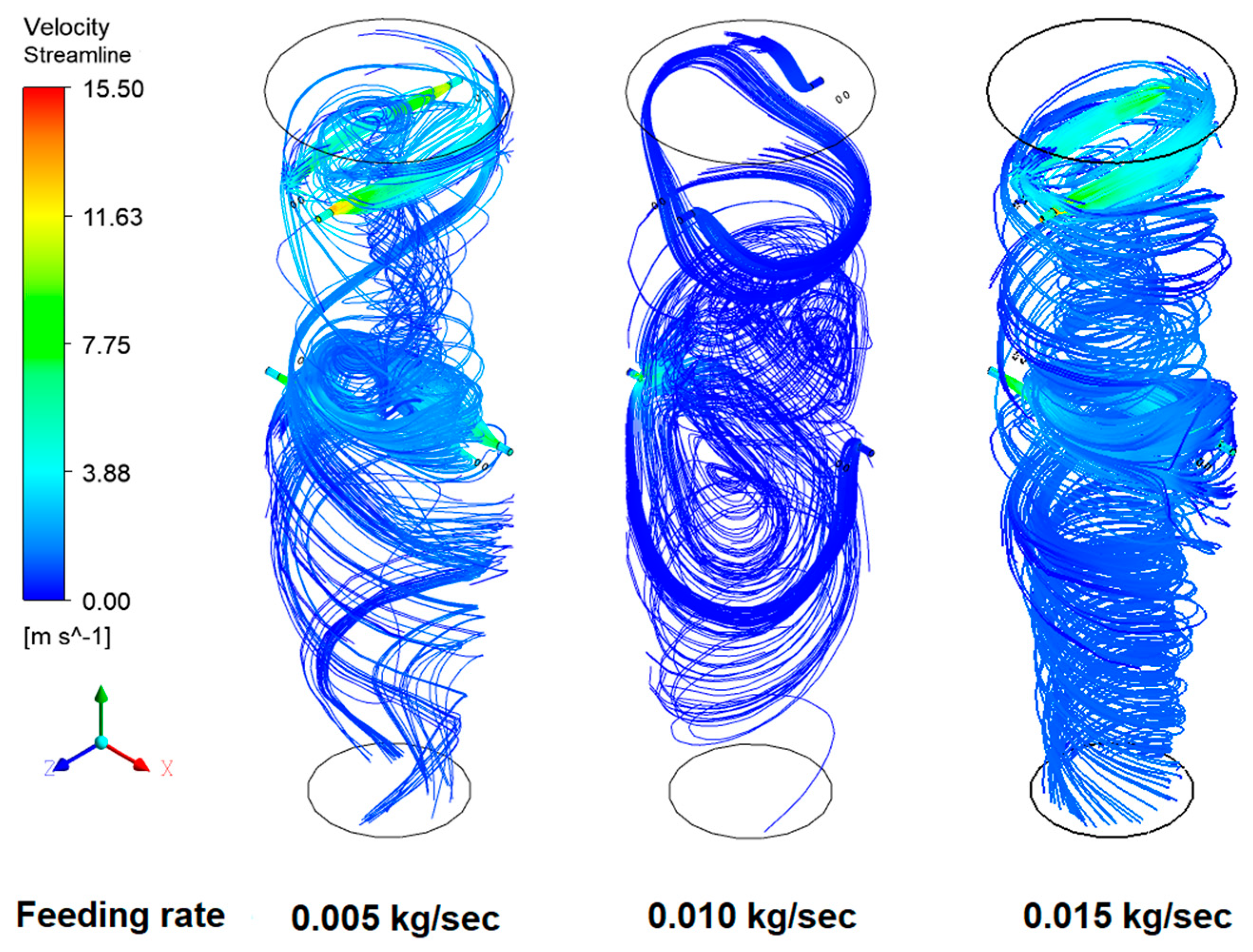
3.7. Flow Visualization
3.8. Comparison of Simulated Results with Published Work
4. Conclusions
Author Contributions
Funding
Data Availability Statement
Acknowledgments
Conflicts of Interest
References
- Akaev, A.; Davydova, O. Climate and Energy: Energy Transition Scenarios and Global Temperature Changes Based on Current Technologies and Trends. In Reconsidering the Limits to Growth: A Report to the Russian Association of the Club of Rome; Springer: Cham, Switzerland, 2023; pp. 53–70. [Google Scholar]
- Zhan, X.; Zhou, Z.; Wang, F. Catalytic effect of black liquor on the gasification reactivity of petroleum coke. Appl. Energy 2010, 87, 1710–1715. [Google Scholar] [CrossRef]
- Jakobs, T.; Djordjevic, N.; Fleck, S.; Mancini, M.; Weber, R.; Kolb, T. Gasification of high viscous slurry R&D on atomization and numerical simulation. Appl. Energy 2012, 93, 449–456. [Google Scholar]
- Shen, C.-H.; Chen, W.-H.; Hsu, H.-W.; Sheu, J.-Y.; Hsieh, T.-H. Co-gasification performance of coal and petroleum coke blends in a pilot-scale pressurized entrained-flow gasifier. Int. J. Energy Res. 2012, 36, 499–508. [Google Scholar] [CrossRef]
- McKendry, P. Energy production from biomass (part 1): Overview of biomass. Bioresour. Technol. 2002, 83, 37–46. [Google Scholar] [CrossRef] [PubMed]
- Umeki, K.; Namioka, T.; Yoshikawa, K. Analysis of an updraft biomass gasifier with high temperature steam using a numerical model. Appl. Energy 2012, 90, 38–45. [Google Scholar] [CrossRef]
- Gani, A.; Zaki, M.; Mamat, R.; Nizar, M.; Rosdi, S.; Yana, S.; Sarjono, R. Analysis of technological developments and potential of biomass gasification as a viable industrial process: A review. Case Stud. Chem. Environ. Eng. 2023, 8, 100439. [Google Scholar]
- Chmielniak, T.; Sciazko, M. Co-gasification of biomass and coal for methanol synthesis. Appl. Energy 2003, 74, 393–403. [Google Scholar] [CrossRef]
- Chen, W.-H.; Wu, J.-S. An evaluation on rice husks and pulverized coal blends using a drop tube furnace and a thermogravimetric analyzer for application to a blast furnace. Energy 2009, 34, 1458–1466. [Google Scholar] [CrossRef]
- Ma, M.; Bai, Y.; Wei, J.; Song, X.; Lv, P.; Wang, J.; Su, W.; Xiong, Q.; Yu, G. Decoupling study of volatile–char interaction during coal/biomass co-gasification based on a two-stage fixed bed reactor: Insight into the role of O-containing compound species. Chem. Eng. Sci. 2023, 265, 118262. [Google Scholar] [CrossRef]
- Chen, W.-H.; Chen, J.-C.; Tsai, C.-D.; Jiang, T.L. Transient gasification and syngas formation from coal particles in a fixed-bed reactor. Int. J. Energy Res. 2007, 31, 895–911. [Google Scholar] [CrossRef]
- Pettinau, A.; Ferrara, F.; Amorino, C. Techno-economic comparison between different technologies for a CCS power generation plant integrated with a sub-bituminous coal mine in Italy. Appl. Energy 2012, 99, 32–39. [Google Scholar] [CrossRef]
- McKendry, P. Energy production from biomass (part 2): Conversion technologies. Bioresour. Technol. 2002, 83, 47–54. [Google Scholar] [CrossRef] [PubMed]
- Srirangan, K.; Akawi, L.; Moo-Young, M.; Chou, C.P. Towards sustainable production of clean energy carriers from biomass resources. Appl. Energy 2012, 100, 172–186. [Google Scholar] [CrossRef]
- Pereira, E.G.; da Silva, J.N.; de Oliveira, J.L.; Machado, C.S. Sustainable energy: A review of gasification technologies. Renew. Sustain. Energy Rev. 2012, 16, 4753–4762. [Google Scholar] [CrossRef]
- Dhrioua, M.; Ghachem, K.; Hassen, W.; Ghazy, A.; Kolsi, L.; Borjini, M.N. Simulation of biomass air gasification in a bubbling fluidized bed using aspen plus: A comprehensive model including tar production. ACS Omega 2022, 7, 33518–33529. [Google Scholar] [CrossRef] [PubMed]
- Guo, F.; Dong, Y.; Dong, L.; Guo, C. Effect of design and operating parameters on the gasification process of biomass in a downdraft fixed bed: An experimental study. Int. J. Hydrogen Energy 2014, 39, 5625–5633. [Google Scholar] [CrossRef]
- Chen, C.; Horio, M.; Kojima, T. Use of numerical modeling in the design and scale-up of entrained flow coal gasifiers. Fuel 2001, 80, 1513–1523. [Google Scholar] [CrossRef]
- Slezak, A.; Kuhlman, J.M.; Shadle, L.J.; Spenik, J.; Shi, S. CFD simulation of entrained-flow coal gasification: Coal particle density/sizefraction effects. Powder Technol. 2010, 203, 98–108. [Google Scholar] [CrossRef]
- Wu, Y.X.; Zhang, J.S.; Yue, G.X.; Lü, J.F. Analysis of the Gasification Performance of a Staged Entrained Flow Gasifier by Presumed PDF Model. Proc. CSEE 2008, 26, 007. [Google Scholar]
- Andries, J.; Becht, J.; Hoppesteyn, P. Pressurized fluidized bed combustion and gasification of coal using flue gas recirculation and oxygen injection. Energy Convers. Manag. 1997, 38, S117–S122. [Google Scholar] [CrossRef]
- Nguyen, T.D.; Ngo, S.I.; Lim, Y.-I.; Lee, J.W.; Lee, U.-D.; Song, B.-H. Three-stage steady-state model for biomass gasification in a dual circulating fluidized-bed. Energy Convers. Manag. 2012, 54, 100–112. [Google Scholar] [CrossRef]
- Vicente, W.; Ochoa, S.; Aguillón, J.; Barrios, E. An Eulerian model for the simulation of an entrained flow coal gasifier. Appl. Therm. Eng. 2003, 23, 1993–2008. [Google Scholar] [CrossRef]
- Gerun, L.; Paraschiv, M.; Vîjeu, R.; Bellettre, J.; Tazerout, M.; Gøbel, B.; Henriksen, U. Numerical investigation of the partial oxidation in a two-stage downdraft gasifier. Fuel 2008, 87, 1383–1393. [Google Scholar] [CrossRef]
- Álvarez, L.; Gharebaghi, M.; Jones, J.; Pourkashanian, M.; Williams, A.; Riaza, J.; Pevida, C.; Pis, J.; Rubiera, F. Numerical investigation of NO emissions from an entrained flow reactor under oxy-coal conditions. Fuel Process. Technol. 2012, 93, 53–64. [Google Scholar] [CrossRef]
- Fletcher, D.; Haynes, B.; Christo, F.; Joseph, S. A CFD based combustion model of an entrained flow biomass gasifier. Appl. Math. Model. 2000, 24, 165–182. [Google Scholar] [CrossRef]
- Ajilkumar, A.; Sundararajan, T.; Shet, U.S.P. Numerical modeling of a steam-assisted tubular coal gasifier. Int. J. Therm. Sci. 2009, 48, 308–321. [Google Scholar] [CrossRef]
- Chui, E.; Majeski, A.; Lu, D.; Hughes, R.; Gao, H.; McCalden, D.; Anthony, E. Simulation of entrained flow coal gasification. Energy Procedia 2009, 1, 503–509. [Google Scholar] [CrossRef]
- Dong, C.; Yang, Y.; Yang, R.; Zhang, J. Numerical modeling of the gasification based biomass co-firing in a 600 MW pulverized coal boiler. Appl. Energy 2010, 87, 2834–2838. [Google Scholar] [CrossRef]
- Chen, C.-J.; Hung, C.-I.; Chen, W.-H. Numerical investigation on performance of coal gasification under various injection patterns in an entrained flow gasifier. Appl. Energy 2012, 100, 218–228. [Google Scholar] [CrossRef]
- Zheng, L.; Furinsky, E. Comparison of Shell, Texaco, BGL and KRW gasifiers as part of IGCC plant computer simulations. Energy Convers. Manag. 2005, 46, 1767–1779. [Google Scholar] [CrossRef]
- Unar, I.N.; Wang, L.; Pathan, A.G.; Mahar, R.B.; Li, R.; Uqaili, M.A. Numerical simulations for the coal/oxidant distribution effects between two-stages for multi opposite burners (MOB) gasifier. Energy Convers. Manag. 2014, 86, 670–682. [Google Scholar] [CrossRef]
- Li, C.; Dai, Z.; Li, W.; Xu, J.; Wang, F. 3D numerical study of particle flow behavior in the impinging zone of an Opposed Multi-Burner gasifier. Powder Technol. 2012, 225, 118–123. [Google Scholar] [CrossRef]
- Ni, J.; Liang, Q.; Zhou, Z.; Dai, Z.; Yu, G. Numerical and experimental investigations on gas–particle flow behaviors of the Opposed Multi-Burner Gasifier. Energy Convers. Manag. 2009, 50, 3035–3044. [Google Scholar] [CrossRef]
- Masmoudi, M.A.; Sahraoui, M.; Grioui, N.; Halouani, K. 2-D Modeling of thermo-kinetics coupled with heat and mass transfer in the reduction zone of a fixed bed downdraft biomass gasifier. Renew. Energy 2014, 66, 288–298. [Google Scholar] [CrossRef]
- Mahmoudi, A.H.; Hoffmann, F.; Peters, B. Application of XDEM as a novel approach to predict drying of a packed bed. Int. J. Therm. Sci. 2014, 75, 65–75. [Google Scholar] [CrossRef]
- Cau, G.; Tola, V.; Pettinau, A. A steady state model for predicting performance of small-scale up-draft coal gasifiers. Fuel 2015, 152, 3–12. [Google Scholar] [CrossRef]
- Patel, K.D.; Shah, N.K.; Patel, R.N. CFD Analysis of Spatial Distribution of Various Parameters in Downdraft Gasifier. Procedia Eng. 2013, 51, 764–769. [Google Scholar] [CrossRef]
- Murgia, S.; Vascellari, M.; Cau, G. Comprehensive CFD model of an air-blown coal-fired updraft gasifier. Fuel 2012, 101, 129–138. [Google Scholar] [CrossRef]
- Wu, Y.; Zhang, Q.; Yang, W.; Blasiak, W. Two-dimensional computational fluid dynamics simulation of biomass gasification in a downdraft fixed-bed gasifier with highly preheated air and steam. Energy Fuels 2013, 27, 3274–3282. [Google Scholar] [CrossRef]
- Ambatipudi, M.K.; Varunkumar, S. A novel MILD gasifier for crushed low-grade solid fuels. Proc. Combust. Inst. 2023, 39, 3479–3488. [Google Scholar] [CrossRef]
- Dhrioua, M.; Hassen, W.; Kolsi, L.; Anbumalar, V.; Alsagri, A.S.; Borjini, M.N. Gas distributor and bed material effects in a cold flow model of a novel multi-stage biomass gasifier. Biomass Bioenergy 2019, 126, 14–25. [Google Scholar] [CrossRef]
- Zhang, Z.; Lu, B.; Zhao, Z.; Zhang, L.; Chen, Y.; Li, S.; Luo, C.; Zheng, C. CFD modeling on char surface reaction behavior of pulverized coal MILD-oxy combustion: Effects of oxygen and steam. Fuel Process. Technol. 2020, 204, 106405. [Google Scholar] [CrossRef]
- Wang, L.; Jia, Y.; Kumar, S.; Li, R.; Mahar, R.B.; Ali, M.; Unar, I.N.; Sultan, U.; Memon, K. Numerical analysis on the influential factors of coal gasification performance in two-stage entrained flow gasifier. Appl. Therm. Eng. 2017, 112, 1601–1611. [Google Scholar] [CrossRef]
- Wen, C.; Chaung, T. Entrainment coal gasification modeling. Ind. Eng. Chem. Process Des. Dev. 1979, 18, 684–695. [Google Scholar] [CrossRef]
- Du, S.-W.; Chen, W.-H.; Lucas, J. Performances of pulverized coal injection in blowpipe and tuyere at various operational conditions. Energy Convers. Manag. 2007, 48, 2069–2076. [Google Scholar] [CrossRef]
- Du, S.-W.; Chen, W.-H. Numerical prediction and practical improvement of pulverized coal combustion in blast furnace. Int. Commun. Heat Mass Transf. 2006, 33, 327–334. [Google Scholar] [CrossRef]
- Maitlo, G.; Unar, I.N.; Mahar, R.B.; Brohi, K.M. Numerical simulation of lignocellulosic biomass gasification in concentric tube entrained flow gasifier through computational fluid dynamics. Energy Explor. Exploit. 2019, 37, 1073–1097. [Google Scholar] [CrossRef]
- Unar, I.N.; Soomro, S.A.; Maitlo, G.; Aziz, S.; Mahar, R.B.; Bhatti, Z.A. Numerical study of coal composition effects on the performance of gasification through computational fluid dynamic. Int. J. Chem. React. Eng. 2019, 17, 20180204. [Google Scholar] [CrossRef]
- Zhang, Z.; Lu, B.; Zhao, Z.; Zhang, L.; Chen, Y.; Luo, C.; Zheng, C. Heterogeneous reactions behaviors of pulverized coal MILD combustion under different injection conditions. Fuel 2020, 275, 117925. [Google Scholar] [CrossRef]
- Skodras, G.; Someus, E.; Grammelis, P.; Palladas, A.; Amarantos, P.; Basinas, P.; Natas, P.; Prokopidou, M.; Diamantopoulou, I.; Kakaras, E.; et al. Combustion and environmental performance of clean coal end products. Int. J. Energy Res. 2007, 31, 1237. [Google Scholar] [CrossRef]
- Macías-García, A.; Cuerda-Correa, E.M.; Díaz-Díez, M.A. Application of the Rosin–Rammler and Gates–Gaudin–Schuhmann models to the particle size distribution analysis of agglomerated cork. Mater. Charact. 2004, 52, 159–164. [Google Scholar] [CrossRef]
- Maitlo, G.; Ali, I.; Mangi, K.H.; Ali, S.; Maitlo, H.A.; Unar, I.N.; Pirzada, A.M. Thermochemical conversion of biomass for syngas production: Current status and future trends. Sustainability 2022, 14, 2596. [Google Scholar] [CrossRef]
- Chanphavong, L.; Al-Attab, K.; Zainal, Z.A. Flameless Combustion Characteristics of Producer Gas Premixed Charge in a Cyclone Combustor. Flow Turbul. Combust. 2019, 103, 731–750. [Google Scholar] [CrossRef]
- Rauch, R.; Hrbek, J.; Hofbauer, H. Biomass gasification for synthesis gas production and applications of the syngas. Wiley Interdiscip. Rev. Energy Environ. 2014, 3, 343–362. [Google Scholar] [CrossRef]
- Minutillo, M.; Perna, A.; Di Bona, D. Modelling and performance analysis of an integrated plasma gasification combined cycle (IPGCC) power plant. Energy Convers. Manag. 2009, 50, 2837–2842. [Google Scholar] [CrossRef]
- Janajreh, I.; Al Shrah, M. Numerical and experimental investigation of downdraft gasification of wood chips. Energy Convers. Manag. 2013, 65, 783–792. [Google Scholar] [CrossRef]
- Janajreh, I.; Raza, S.S.; Valmundsson, A.S. Plasma gasification process: Modeling, simulation and comparison with conventional air gasification. Energy Convers. Manag. 2013, 65, 801–809. [Google Scholar] [CrossRef]
- Luan, Y.-T.; Chyou, Y.-P.; Wang, T. Numerical analysis of gasification performance via finite-rate model in a cross-type two-stage gasifier. Int. J. Heat Mass Transf. 2013, 57, 558–566. [Google Scholar] [CrossRef]
- Vascellari, M.; Arora, R.; Pollack, M.; Hasse, C. Simulation of entrained flow gasification with advanced coal conversion submodels. Part 1: Pyrolysis. Fuel 2013, 113, 654–669. [Google Scholar] [CrossRef]
- Vascellari, M.; Arora, R.; Hasse, C. Simulation of entrained flow gasification with advanced coal conversion submodels. Part 2: Char conversion. Fuel 2014, 118, 369–384. [Google Scholar] [CrossRef]
- Troiano, M.; Santagata, T.; Montagnaro, F.; Salation, P. Impact experiments of char and ash particles relevant to entrained-flow coal gasifiers. Fuel 2017, 202, 665–674. [Google Scholar] [CrossRef]
- Unar, I.N. Kinetic Modeling of Gasification Reactions for Lignite Coal Under High Pressure. Ph.D. Thesis, Mehran University of Engineering & Technology, Jamshoro, Pakistan, 2018. [Google Scholar]


| Sr. No | Specification | Value |
|---|---|---|
| 1 | Diameter of main gasifier body | 350 mm |
| 2 | Height | 1200 mm |
| 3 | Diameter of inlet nozzles | 10 mm |
| 4 | Outlet diameter | 230 mm |
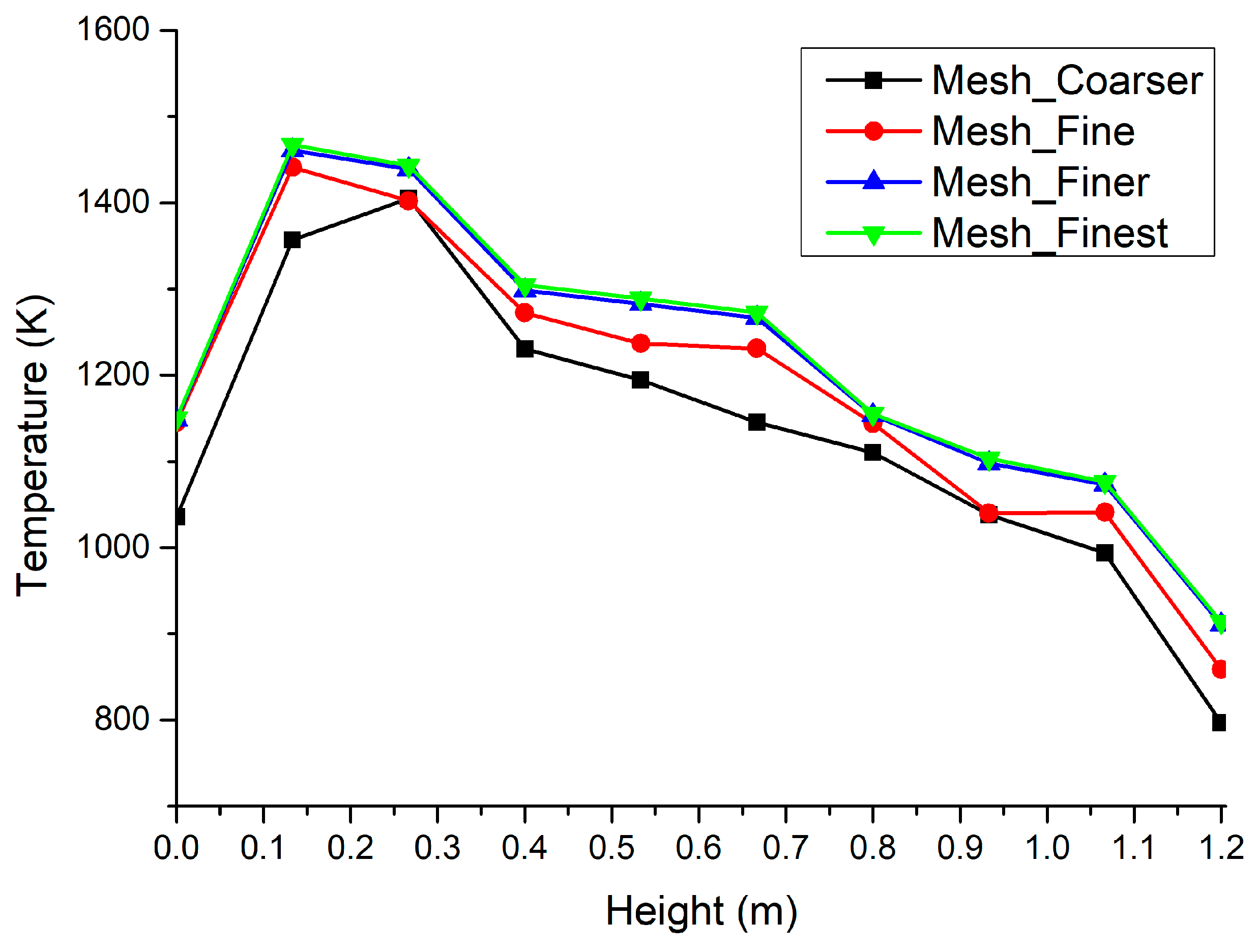
| Sr. No | Grid Name | No. of Elements |
|---|---|---|
| 1 | Coarser mesh | 78,457 |
| 2 | Fine mesh | 89,748 |
| 3 | Finer mesh | 112,185 |
| 4 | Finest mesh | 185,850 |
| Physics | Governing Equations | Equation No. |
|---|---|---|
| Continuity | (1) | |
| Momentum | (2) | |
| Energy | (3) | |
| Species transport model | (4) | |
| Kinematic viscosity | (5) | |
| Kinetic energy | (6) | |
| Dissipation rate | (7) | |
| Heat conductivity | (8) | |
| Diffusion coefficient | (9) | |
| Discrete phase model | ||
| Change in velocity of a particle | (10) | |
| Drag force | (11) | |
| Constants | = 0.09 = 1.44 = 1.92 = 1.0 = 1.3 = 0.85 = 0.7 | |
| Parameter | Value |
|---|---|
| 1.28 × 10⁷ | |
| 200,000 | |
| 1 | |
| 0.29 | |
| 165.3 | |
| 106.9 |
| Sr. No | Reactions | Schemes | Kinetic Parameters | ||||||
|---|---|---|---|---|---|---|---|---|---|
| A | B | C | D | E | F | A (Pre-Exponent Factor) | E (Activation Energy) | ||
| Homogeneous Reactions | |||||||||
| 1 * | Vol + X O2 → A CO2 + B H2O + C N2 + D SO2 (Volatiles complete combustion) | 2.119 × 10¹¹ | 2.03 × 10⁸ | ||||||
| 2 * | Vol + X’ O2 → A’ CO + B H2O + C N2 + D SO2 (Volatiles partial combustion) | 2.12 × 10¹¹ | 2.20 × 10¹¹ | ||||||
| 3 | (CO combustion) | 2.239 × 10¹² | 1.70 × 10⁸ | ||||||
| 4 | (H2 combustion) | 6.800 × 10¹⁵ | 1.68 × 10⁸ | ||||||
| 5 | (Water shift reaction) (f) | 2.750 × 10¹⁰ | 8.38 × 10⁷ | ||||||
| 6 | (Water shift reaction) (b) | 0.0265 | 3960 | ||||||
| Heterogeneous Reactions | |||||||||
| 7 | (Char partial combustion) | 0.052 | 6.10 × 10⁷ | ||||||
| 8 | (Char complete combustion) | 415.7 | 9.04 × 10⁷ | ||||||
| 9 | (Gasification, Boudourad reaction) | 107,800 | 2.44 × 10⁷ | ||||||
| 10 | (Gasification) | 97,540 | 2.02 × 10⁸ | ||||||
| Biomass Type | Lakhra Coal | Rice Husk | Wood Sawdust |
|---|---|---|---|
| Proximate analysis (wt.%, dry basis) | |||
| M | 9.93 | 4.83 | 5.53 |
| VM | 43.69 | 61.86 | 72.60 |
| FC | 31.96 | 15.30 | 14.55 |
| Ash | 14.42 | 18.01 | 7.32 |
| Ultimate analysis (wt. %, dry basis) | |||
| C | 67.84 | 45.8 | 44.1 |
| H | 7.9 | 6 | 5.96 |
| N | 1.43 | 0.3 | 0.36 |
| O | 13.81 | 47.9 | 49.39 |
| S | 9.02 | 0 | 0.19 |
| HHV (J kg−1) | 1.89 × 10⁷ | 1.33 × 10⁷ | 1.88 × 10⁷ |
| Sr. No | Case Name | Feedstock | Feeding Rate | O/C Ratio | Oxidant Flowrate | Oxidant Distribution (kg/s) | |
|---|---|---|---|---|---|---|---|
| (kg/s) | (kg/s) | Up-Nozzles (60%) | Down-Nozzles (40%) | ||||
| 1 | LC_0.005_0.9 | LC | 0.005 | 0.9 | 0.0024 | 0.00072 | 0.00048 |
| 2 | LC_0.005_1.0 | LC | 0.005 | 1.0 | 0.0027 | 0.00081 | 0.00054 |
| 3 | LC_0.005_1.1 | LC | 0.005 | 1.1 | 0.003 | 0.0009 | 0.0006 |
| 4 | LC_0.01_0.9 | LC | 0.01 | 0.9 | 0.0047 | 0.00141 | 0.00094 |
| 5 | LC_0.01_1.0 | LC | 0.01 | 1.0 | 0.0054 | 0.00162 | 0.00108 |
| 6 | LC_0.01_1.1 | LC | 0.01 | 1.1 | 0.0061 | 0.00183 | 0.00122 |
| 7 | LC_0.015_0.9 | LC | 0.015 | 0.9 | 0.0071 | 0.00213 | 0.00142 |
| 8 | LC_0.015_1.0 | LC | 0.015 | 1.0 | 0.0081 | 0.00243 | 0.00162 |
| 9 | LC_0.015_1.1 | LC | 0.015 | 1.1 | 0.0091 | 0.00273 | 0.00182 |
| 10 | RH_0.005_0.9 | RH | 0.005 | 0.9 | 0.0206 | 0.00618 | 0.00412 |
| 11 | RH_0.005_1.0 | RH | 0.005 | 1.0 | 0.0229 | 0.00687 | 0.00458 |
| 12 | RH_0.005_1.1 | RH | 0.005 | 1.1 | 0.0252 | 0.00756 | 0.00504 |
| 13 | RH_0.01_0.9 | RH | 0.01 | 0.9 | 0.0041 | 0.00123 | 0.00082 |
| 14 | RH_0.01_1.0 | RH | 0.01 | 1.0 | 0.0458 | 0.01374 | 0.00916 |
| 15 | RH_0.01_1.1 | RH | 0.01 | 1.1 | 0.0504 | 0.01512 | 0.01008 |
| 16 | RH_0.015_0.9 | RH | 0.015 | 0.9 | 0.0618 | 0.01854 | 0.01236 |
| 17 | RH_0.015_1.0 | RH | 0.015 | 1.0 | 0.0687 | 0.02061 | 0.01374 |
| 18 | RH_0.015_1.1 | RH | 0.015 | 1.1 | 0.0756 | 0.02268 | 0.01512 |
| 19 | WS_0.005_0.9 | WS | 0.005 | 0.9 | 0.002 | 0.0006 | 0.0004 |
| 20 | WS_0.005_1.0 | WS | 0.005 | 1.0 | 0.0022 | 0.00066 | 0.00044 |
| 21 | WS_0.005_1.1 | WS | 0.005 | 1.1 | 0.0024 | 0.00072 | 0.00048 |
| 22 | WS_0.01_0.9 | WS | 0.01 | 0.9 | 0.004 | 0.0012 | 0.0008 |
| 23 | WS_0.01_1.0 | WS | 0.01 | 1.0 | 0.0044 | 0.00132 | 0.00088 |
| 24 | WS_0.01_1.1 | WS | 0.01 | 1.1 | 0.0049 | 0.00147 | 0.00098 |
| 25 | WS_0.015_0.9 | WS | 0.015 | 0.9 | 0.006 | 0.0018 | 0.0012 |
| 26 | WS_0.015_1.0 | WS | 0.015 | 1.0 | 0.0066 | 0.00198 | 0.00132 |
| 27 | WS_0.015_1.1 | WS | 0.015 | 1.1 | 0.0073 | 0.00219 | 0.00146 |
Disclaimer/Publisher’s Note: The statements, opinions and data contained in all publications are solely those of the individual author(s) and contributor(s) and not of MDPI and/or the editor(s). MDPI and/or the editor(s) disclaim responsibility for any injury to people or property resulting from any ideas, methods, instructions or products referred to in the content. |
© 2023 by the authors. Licensee MDPI, Basel, Switzerland. This article is an open access article distributed under the terms and conditions of the Creative Commons Attribution (CC BY) license (https://creativecommons.org/licenses/by/4.0/).
Share and Cite
Rehman, A.u.; Unar, I.N.; Abro, M.; Qureshi, K.; Almani, S.; Jatoi, A.S. Numerical Simulations of Gasification of Low-Grade Coal and Lignocellulosic Biomasses in Two-Stage Multi-Opposite Burner Gasifier. Processes 2023, 11, 3451. https://doi.org/10.3390/pr11123451
Rehman Au, Unar IN, Abro M, Qureshi K, Almani S, Jatoi AS. Numerical Simulations of Gasification of Low-Grade Coal and Lignocellulosic Biomasses in Two-Stage Multi-Opposite Burner Gasifier. Processes. 2023; 11(12):3451. https://doi.org/10.3390/pr11123451
Chicago/Turabian StyleRehman, Anees u, Imran Nazir Unar, Masroor Abro, Khadija Qureshi, Sikandar Almani, and Abdul Sattar Jatoi. 2023. "Numerical Simulations of Gasification of Low-Grade Coal and Lignocellulosic Biomasses in Two-Stage Multi-Opposite Burner Gasifier" Processes 11, no. 12: 3451. https://doi.org/10.3390/pr11123451
APA StyleRehman, A. u., Unar, I. N., Abro, M., Qureshi, K., Almani, S., & Jatoi, A. S. (2023). Numerical Simulations of Gasification of Low-Grade Coal and Lignocellulosic Biomasses in Two-Stage Multi-Opposite Burner Gasifier. Processes, 11(12), 3451. https://doi.org/10.3390/pr11123451