Dynamic Job-Shop Scheduling Based on Transformer and Deep Reinforcement Learning

Abstract

The dynamic job-shop scheduling problem is a complex and uncertain task that involves optimizing production planning and resource allocation in a dynamic production environment. Traditional methods are limited in effectively handling dynamic events and quickly generating scheduling solutions; in order to solve this problem, this paper proposes a solution by transforming the dynamic job-shop scheduling problem into a Markov decision process and leveraging deep reinforcement learning techniques. The proposed framework introduces several innovative components, which make full use of human domain knowledge and machine computing power, to realize the goal of man–machine collaborative decision-making. Firstly, we utilize disjunctive graphs as the state representation, capturing the complex relationships between various elements of the scheduling problem. Secondly, we select a set of dispatching rules through data envelopment analysis to form the action space, allowing for flexible and efficient scheduling decisions. Thirdly, the transformer model is employed as the feature extraction module, enabling effective capturing of state relationships and improving the representation power. Moreover, the framework incorporates the dueling double deep Q-network with prioritized experience replay, mapping each state to the most appropriate dispatching rule. Additionally, a dynamic target strategy with an elite mechanism is proposed. Through extensive experiments conducted on multiple examples, our proposed framework consistently outperformed traditional dispatching rules, genetic algorithms, and other reinforcement learning methods, achieving improvements of 15.98%, 17.98%, and 13.84%, respectively. These results validate the effectiveness and superiority of our approach in addressing dynamic job-shop scheduling problems.

1. Introduction

With the development of economic globalization, manufacturing industries are facing fierce market competition. Production scheduling plays a central role in the manufacturing process, and the traditional shop scheduling problem is static and deterministic, which is suitable for a single production environment and mode. However, with the development of acquisition hardware and the advancement of processing technology, the scheduling events in a workshop can be captured in real-time, which puts forward higher requirements for the real-time response of scheduling, making it a challenging task to quickly obtain high-quality scheduling schemes.

The machining sequence of workpieces in a workshop is constrained by multiple criteria, which is a typical combinatorial optimization problem. When the number of machines is greater than two, this kind of problem is proven to be non-deterministic polynomial-time hard (NP-hard) [1]. However, in the existing solutions for job-shop scheduling problems, the accurate algorithm is only suitable for small-scale problems and has no advantage in calculation time, which is not suitable for dynamic scheduling. In addition, the swarm intelligence algorithm cannot generate the optimal solution in a reasonable calculation time and cannot deal with the complex uncertainties of a workshop. Furthermore, dispatching rules [2] have low time complexity in the process of solving and can handle the dynamic changes of the workshop but lack adaptive adjustment ability. So far, due to the different actual production conditions and the different scale of scheduling problems, no algorithm is completely superior to one algorithm, and most methods have low adaptability and strong subjectivity and can only be applied to the current production environment.

In order to solve the above problems, researchers began to apply reinforcement learning [3] to the study of job-shop scheduling. Some scholars adopted reinforcement learning algorithms based on value functions to solve job-shop scheduling problems. Samsonov et al. [4] proposed an action space independent of the problem dimension, which is independent of the number of machines and orders and is applicable to both discrete and continuous action spaces. In addition, a new reward mechanism was introduced to obtain the optimal solution through a higher reward gradient. Bouazza et al. [5] decomposed job-shop scheduling into machine allocation problems and job allocation problems and proposed a new type of reward shaping in which the action space is divided into machine allocation rules and job selection rules. Experiments showed that the scheduling performance was improved by 27% compared with the usual heuristic method. In addition to single-agent learning, reinforcement learning also includes multi-agent learning. He et al. [6] proposed a multi-agent reinforcement learning (MARL) framework that transformed the optimization process into a random game and introduced a deep Q-network algorithm to train multi-agents. In each state, the interruption of a multiple equilibrium is avoided so as to achieve the relevant equilibrium optimal solution of the optimization process. In addition, Wang et al. [7] proposed an algorithm for job-shop scheduling in a resource preemption environment using multiple agents to learn the decision-making strategy of each agent and the cooperation between agents. Lang et al. [8] trained two DQN agents, one to select the sequence of operations and the other to select the assignment of work to the machine, which, combined with a discrete event simulation model of the problem, were able to quickly predict and evaluate new scheduling schemes in less than 0.2 s.

Job-shop scheduling is highly complex, and using reinforcement learning alone has some shortcomings, such as slow convergence, easy falling into local optimal solutions, etc. Therefore, many researchers have combined reinforcement learning with other algorithms to solve the above problems. Chen et al. [9] proposed a self-learning genetic algorithm (SLGA) that takes the genetic algorithm as the basic optimization method and uses reinforcement learning to intelligently adjust its key parameters. Experiments showed that the learning effect and performance of the algorithm were significantly better than that of similar algorithms. Junyoung Park et al. [10] proposed a framework using a graph neural network and reinforcement learning to solve the scheduling job-shop problem, using the GNN to learn the node features embedded in the spatial structure, and mapping the features to the best actions to obtain the optimal scheduling strategy. They empirically demonstrated that the GNN scheduler outperformed the favored dispatching rules and RL-based schedulers on various benchmark JSSPs.

The scheduling of a static job shop is predetermined, unable to flexibly respond to changing production needs, and the environmental conditions’ lack of flexibility, the occurrence of equipment failure, and other dynamic factors will interfere with the original plan, resulting in low production efficiency and a waste of resources. Therefore, researchers began to study reinforcement learning algorithms based on the value function to solve job-shop scheduling problems under dynamic perturbations; in recent years, deep learning and reinforcement learning have been combined to form the field named deep reinforcement learning [11] which can make comprehensive real-time responses to dynamic events. Table 1 shows some existing methods for DRL-based dynamic job-shop scheduling.

Aiming at the dynamic job-shop scheduling problem (DJSP) of machine failure, Bar et al. [12] proposed a method to solve the dynamic job-shop scheduling problem by combining multi-agents and DQN. Multiple agents share an experience pool and cooperate through reinforcement learning, and each agent considers each other’s requirements to optimize the overall goal. Zhao et al. [13] proposed an improved Q-learning algorithm in which the agent can simultaneously select the operation to be processed and the executing machine when the machine fails, with the initial scheduling scheme being formulated by a genetic algorithm. The experimental results showed that this method can effectively reduce the operation delay time.

Aiming at the dynamic scheduling job-shop problem of the random arrival of new jobs, Luo et al. [14] proposed a double-loop DQN algorithm, DLDQN, which combines the exploration cycle and the exploitation cycle and has both global exploration and local convergence capabilities. Experimental results showed that DLDQN performed better than deep reinforcement learning based on standard Q-learning and dispatching rules. In addition, Turgut et al. [15] applied DQN to solve the job-shop scheduling problem, with the goal of minimizing job delay time, and compared it with two common dispatching rules (minimum processing time and earliest due date) to further verify the performance of the model. Chang et al. [16] proposed a double DQN (DDQN) architecture to solve the dynamic flexible job-shop scheduling problem (DFJSP), and experimental results showed that this method was superior to other reinforcement learning algorithms in terms of solution quality and generalization. In addition, Wang et al. [17] constructed a dynamic scheduling system model based on multiple agents, set machine, buffer, state, and job as agents, used weighted Q-learning to determine the processing order of jobs on the machine, defined four state features, reduced the dimension of state space by clustering, and proposed a dynamic greedy search strategy to avoid the blind search of traditional strategies. Bouazza et al. [5] used a Q-learning algorithm to solve part of the flexible job-shop scheduling problem with new job insertion where one Q matrix is used to select machine selection rules and the other Q matrix is used to select specific scheduling rules. Shahrabi et al. [18] obtained the appropriate VNS parameters at any rescheduling point and used the Q-learning algorithm for reinforcement learning. In this method, the action is selected using the e-greedy policy based on the workshop condition defined as the state. It significantly improved the performance of scheduling methods. The proposed method not only solved the dynamic nature of the actual production environment but also dynamically updated the optimization strategy.

Aiming at the dynamic scheduling workshop problem of new job insertion, Luo et al. [19] extracted seven general features, with values from 0 to 1 to represent the state of each rescheduling point, and proved the superiority of DQN in comparing each combination rule, distributed rule and standard Q-learning through experiments. In addition, Luo et al. [20] also proposed a two-layer DQN online rescheduling framework which included two DQN-based agents. The upper DQN is used to control the temporary optimization objectives of the lower DQN, and at each rescheduling point, the behavior of the lower DQN is guided according to the current state characteristics. The lower DQN takes the state characteristics and the optimization objectives passed from the upper DQN as inputs and selects feasible dispatching rules by calculating the Q value of each scheduling rule. The effectiveness and universality of the proposed THDQN were proved by experiments.

In addition to directly using scheduling rules, custom rules, and scheduling operations as action spaces, some researchers chose to use tools to select the scheduling rules based on evidence, which can be more in line with the scheduling production environment and greatly improve scheduling efficiency. For example, Marcello Braglia et al. [21] used data enveloping analysis (DEA) to measure and compare the performance of scheduling rules according to several possible evaluation criteria. Amar Oukil et al. [22] proposed a scheduling rule ranking method for a multi-objective dynamic flow shop scheduling system based on data envelopment analysis and a basic scheduling strategy that can switch between different preferred rules according to the average deadline closeness of the current work portfolio in the shop. In addition, he proposed an integrated data envelopment analysis (DEA) and ordered weighting average (OWA) model [23], which was applied to 28 scheduling rules for scheduling jobs that continuously reach random time points in the production cycle. The calculation results highlighted the influence of energy cost on the overall ranking of scheduling rules and revealed the superiority of some rules under multi-objective performance criteria, whose application background is energy-saving scheduling. It can be seen that, based on the simulation data of the dynamic job-shop scheduling rules studied in the above literature, the DEA method is suitable for sorting competitive scheduling rules according to a selected set of performance criteria and plays a great auxiliary role in the selection of scheduling rules.

Table 1. The reinforcement learning algorithm based on the value function solves the dynamic job-shop scheduling problem.

Work	State Representation	Action Space	Dynamic Factors	Problems	Objective	Algorithm
Turgut et al. [15]	Matrix	Eligible operations	Random job arrival	DJSP	Tardiness	DQN
Chang et al. [16]	Self-designed	Self-designed rules	Random job arrival	DFJSP	Earliness penalty and tardiness	DDQN
Wang et al. [17]	Matrix	Dispatching rules	Random job arrival	DJSP	Premature completion and tardiness	Q-learning
Bouazza et al. [5]	Vector	Dispatching rules	Random job arrival	DFJSP	Makespan and total weighted completion time	Q-learning
Luo et al. [19]	Matrix	Operations	Random job arrival	DFJSP	Tardiness	DDQN
Luo et al. [20]	Matrix	Self-designed rules	Random job arrival	DJSP	Tardiness and utilization rate of machine	DDQN
Shahrabi et al. [18]	Variables	Actions	Random job arrival	DJSP	Mean flow time	Q-learning
Ours	Transformer	Dispatching rules-DEA	Random job arrival	DJSP	Makespan	D3QPN

Table 1. The reinforcement learning algorithm based on the value function solves the dynamic job-shop scheduling problem.

Work	State Representation	Action Space	Dynamic Factors	Problems	Objective	Algorithm
Turgut et al. [15]	Matrix	Eligible operations	Random job arrival	DJSP	Tardiness	DQN
Chang et al. [16]	Self-designed	Self-designed rules	Random job arrival	DFJSP	Earliness penalty and tardiness	DDQN
Wang et al. [17]	Matrix	Dispatching rules	Random job arrival	DJSP	Premature completion and tardiness	Q-learning
Bouazza et al. [5]	Vector	Dispatching rules	Random job arrival	DFJSP	Makespan and total weighted completion time	Q-learning
Luo et al. [19]	Matrix	Operations	Random job arrival	DFJSP	Tardiness	DDQN
Luo et al. [20]	Matrix	Self-designed rules	Random job arrival	DJSP	Tardiness and utilization rate of machine	DDQN
Shahrabi et al. [18]	Variables	Actions	Random job arrival	DJSP	Mean flow time	Q-learning
Ours	Transformer	Dispatching rules-DEA	Random job arrival	DJSP	Makespan	D3QPN

In summary, when solving dynamic job-shop scheduling problems, the existing methods rely on the knowledge and experience of domain experts in setting state characteristics and action spaces, which leads to the fact that they are easily affected by subjective factors in the actual production process. Moreover, some studies lack comparative experiments with other reinforcement learning methods and do not have the ability of adaptive adjustment; therefore, it is difficult to judge whether the scheduling effect is good. Thus, this paper proposes a dynamic job-shop scheduling method based on deep reinforcement learning combined with a transformer, and its contributions are as follows:

(1)

This paper proposes an innovative deep reinforcement learning framework to solve the scheduling problem of both static and dynamic events. Taking the disjunctive graph as a state space, and using the transformer model to extract graph features, the state is mapped to the most appropriate dispatching rules through the double dueling Q-network with prioritized experience replay (D3QPN) which can select the job with the highest priority to execute. A reward function equivalent to minimizing the makespan is designed to evaluate the scheduling results.

(2)

This paper uses data envelopment analysis to select the appropriate dispatching rules from the general dispatching rules to compose the action space, aiming at minimizing the makespan and maximizing machine utilization. It also proposes a dynamic target strategy with an elite strategy, in which an objective function $\mathcal{L}$ with values between 0 and 1 is introduced. The experimental results show that the scheduling performance is improved by 15.93% under this strategy.

(3)

Taking the OR-Library as the dataset, this paper comprehensively compares the proposed method with various dispatching rules, the genetic algorithm (GA), and other reinforcement learning methods. The experimental results show that the proposed method reaches the best level of scheduling effect compared with other methods.

The rest of this paper is organized as follows: Section 2 gives the problem formulation and establishes the mathematical model of DJSP; Section 3 introduces the methodology and gives the details of the proposed method; Section 4 provides the results of numerical experiments; and Section 5 draws a conclusion.

2. Problem Formulation

2.1. DJSP Description

Dynamic job-shop scheduling refers to a process in which multiple jobs need to be processed on multiple machines in a workshop. The processing sequence of these jobs, and the allocation of machines, needs to have scheduling decisions made according to real-time situations and constraints. The dynamic job-shop scheduling problem (DJSP) is a classic combinatorial optimization problem. Its goal is to minimize the job makespan and optimize resource utilization through a reasonable scheduling strategy. Factors such as job sorting and the constraints between machines can be uncertain and dynamic, leading to complexity in scheduling problems.

We describe the dynamic flexible job-shop scheduling problem with random job arrival using the symbols defined as follows: suppose there are n successively arriving jobs $J=\{J_1,J_2\dots J_n\}$ and m machines in the workshop $m=\{M_1,M_2\dots M_m\}$, with each job having k operations to be processed. The job $J_i$ operation sequence is then defined as $O_i=\{O_{i1},O_{i2}\dots O_{ik}\}$ and the machine matrix is $M=\left\{M_{il}\right|M_{il}=0,M_1,M_2\dots M_m\left\}\right(i=\mathrm{1,2},\dots ,n , l=\mathrm{1,2},\dots ,k)$, indicating that $O_{il}$ should be handled by $M_{il}$; the processing time matrix is ${ T}_{il}\ge 0 (i=\mathrm{1,2},\dots ,n , l=\mathrm{1,2},\dots ,k)$, which represents the time required to process $O_{il}$, if $M_{il}$ = 0, then $T_{il}$ = 0, indicating that job $J_i$ does not need to process operation $O_{il}$. This paper takes minimizing the makespan as the scheduling goal, that is $min\left\{C_{max}\right\}$.

$$C_{max}=\max \left({\mathrm{C}}_{i(l-1)},{\mathrm{C}}_{lastO}\right)+{\mathrm{T}}_w+{\mathrm{T}}_{il}$$

(1)

where $C_{il}$ is the completion time of the operation $O_{il}$ on the machine $M_{il}$, which consists of three parts, namely, ${\mathrm{C}}_{i(l-1)}$ the completion time of the previous operation of the same job, ${\mathrm{C}}_{lastO}$ the completion time of the previous operation on the same machine, and ${\mathrm{T}}_w$ the waiting time when the machine is idle (in most cases, it is ineffective and negligible).

The processing time of each operation in the workshop is set, the processing machine for each operation is specified, and, before any dynamic events occur, the processing is carried out according to the specified process route. Note the following points:

(1)

Each machine can only perform one operation every time;

(2)

Each operation of the job can only be performed by one machine every time;

(3)

All operations of the same job must be performed in a predetermined order;

(4)

An operation that has been started cannot be interrupted or terminated;

(5)

The conversion time and setup time between machines are ignored.

2.2. MDP Formulation for DJSP

The goal of DJSP is to determine the order of operations in a dynamic environment, which is essentially a sequential decision problem. This paper formulates it as Markov decision process (MDP), which was originally proposed by Richard Bellman [24] in the 1950s. It is composed of a state set S, behavior set A, state transition probability matrix, reward function R, and discount factor $\gamma$, as shown in Equation (2). At each step of the state transition, the agent can choose one of several possible actions, and the transition probability depends on the chosen action.

$$MDP=(S,A,P,R,\gamma )$$

(2)

The state set $S=S_1,S_2\dots S_t$ represents the set of various possible states, including the features related to the environment and scheduling goals. The state $S_t$ at any time will become a specific state contained in the state set $S$. The action set $A=a_1,a_2\dots a_t$ represents the set of all actions that the agent can perform. The state transition probability $P_{s,s^{\prime }}^a$ represents the probability of changing to state $s^{\prime }$ when the agent takes action $a$ in state $s$. The reward function $R_s^a$ is used to return the reward expectation value when performing action $a$ under state $s$, which is set according to the scheduling goal. The discount factor is used to measure the importance of future rewards, with values ranging from 0 to 1, and is used to balance the weight of current and future rewards.

2.3. Disjunctive Graph

The disjunctive graph model [25] is a general expression method for scheduling problems which can be combined with deep reinforcement learning to deeply mine data and promote more scientific decision-making. The disjunctive graph is a directed graph $G=(V, C\cup D)$, where $V$ is the set of operational vertices, containing two virtual vertices representing the start and end, and their processing time is zero; $C$ is the combinatorial arc, representing the priority constraint relationship between two consecutive operations in the same job; and $D$ consists of undirected disjunctive edges connected to mutually disordered tasks performed on the same machine. 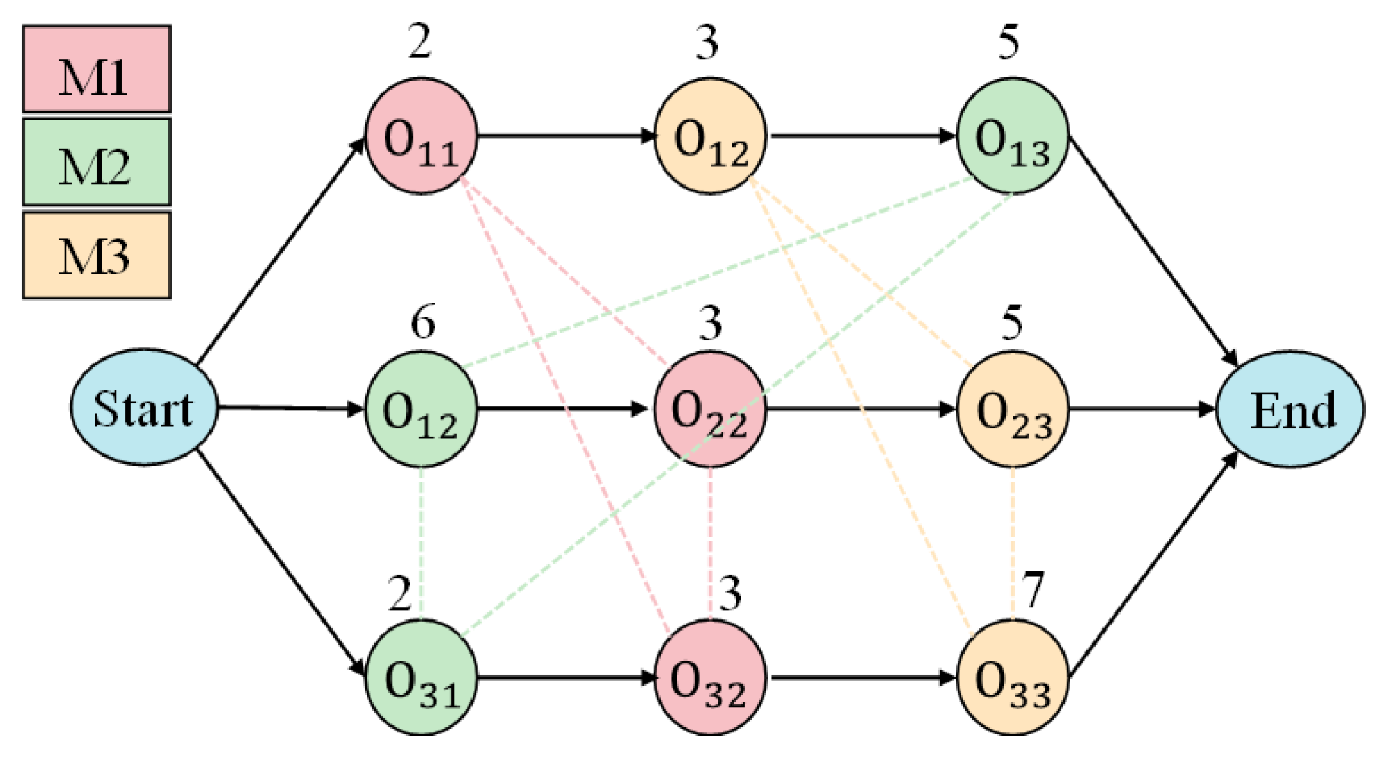Figure 1 shows an example of a simple disjunctive graph, where each circle represents an operation with its name and processing time. Operating vertices on the same machine are represented by the same color, with the solid and dashed arrows representing conjunctive and disjunctive arcs, respectively. The initial state is unsolved and needs to be scheduled by transforming each undirected disjunctive edge into a directed conjunctive edge. Determining the direction of all disjunctive edges decides the processing order of all competing tasks on the same machine. When the disjunctive graph becomes an acyclic graph, a feasible scheduling scheme is obtained.

Generally, disjunctive graphs contain only static information, such as machine sharing and operation priority, but not dynamic information. In order to solve the dynamic scheduling problem, this paper defines the vertex features of disjunctive graphs based on dynamic scheduling, including the following: 1. Job $id$: Indicates the job identifier to which the operation belongs; 2. Operation sequence $id$: Indicates the operation identifier; 3. Node state: Indicates the status of the operation node (incomplete, processing, and completed); 4. Machine $id$: Indicates the identifier of the machine that can perform the operation; 5. Waiting time: Indicates the waiting time between the start of the job and the time when the operation can be performed. 6. Number of remaining operations: Indicates the number of remaining operations to be performed in the job; and 7. Completion rate: Indicates the completion rate of the entire job when the operation is completed. By introducing these dynamic features, key information such as the job execution state, machine assignment, and job completion can be provided to describe the vertex information more comprehensively so as to better support the analysis and decision-making of dynamic scheduling.

The overall idea of the disjunction-based scheduling scheme is to first initialize the dataset, assign the task with the highest priority to the available machines, and remove the task from the task set, while adding the subsequent operations of the task to the task set, and repeat the process until all the task sets are empty, that is, all the tasks have been scheduled to complete. In this way, tasks can be assigned and executed in order of priority and operation, minimizing the waiting time for jobs and achieving efficient scheduling.

3. Methodology

3.1. Overall Framework

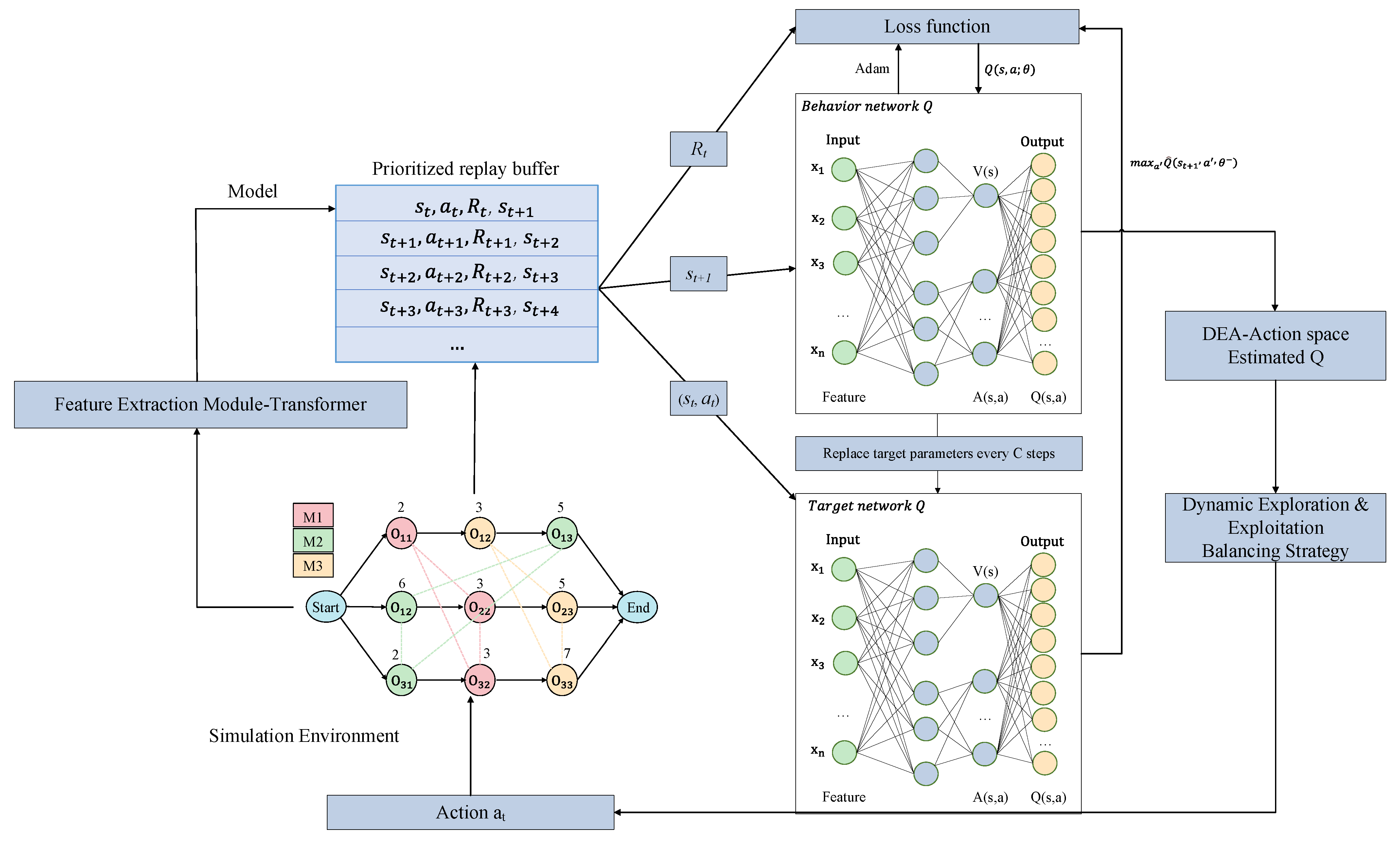
This paper proposes a framework, shown in Figure 2, which combines deep reinforcement learning based on value functions and disjunctive graphs to transform the scheduling problem into a sequential decision problem by defining the environment, state, action, reward, and strategy. As shown in Algorithm 1, optimal scheduling schemes can be solved by learning and optimizing the strategy. The advantage of this framework is that it can make full use of the ability of deep reinforcement learning for decision learning and combine the characteristics of disjunctive graphs to describe and solve scheduling problems.

The traditional state representation methods usually use discrete or continuous features to represent the state information of the workpiece, machine, time, etc., resulting in a high dimension of the state space, which increases the complexity of the calculation and search. There are some defects such as the dimension disaster, difficulty in feature selection, inability to adequately express the accurate value of the state, information loss, and so on. In view of the above problems, this paper adopts a more advanced representation method to model the scheduling environment, that is, a disjunctive graph. This models the shop scheduling problem in a structured way, representing jobs, machines, and processes as nodes in the diagram to capture the long-term dependence relationship between jobs, has high adaptability and scalability to better capture the relationship between states and dynamic changes, and provides a more flexible, accurate, and adaptable state representation.

In this paper, each state is mapped to the most suitable scheduling rule through D3QPN, and the job with the highest priority is selected from the current job. After the action is executed, the disjunctive graph state is updated in real-time, and the experience is stored in the experience pool in the form of a quadruple. Experience is put into the network through the prioritized experience replay mechanism during training until the set epoch is reached.

Algorithm 1 Proposed framework D3QPN and transformer

Input: Environment and set of network random variables

1. Initialize Feature Extraction module; replay buffer; prioritized replay exponent; minibatch

2. Formularize the DJSP as MDP $MDP=\left(S,A,P,R,\gamma \right)$

3. for epoch number $epoch=\mathrm{1,2},\dots ,max\_epoch$ do

4.  Extract the statest from s using Feature Extraction module

5.  Select the dispatching rule using DEA

6.  for schedule cycle $i=\mathrm{1,2},\dots k$ do

7.   Execute dispatching rule $a_t$ and observe new disjunctive graph $s_t$

8.   Execute the state $s_{t+1}$ from $s_t$

9.  end for

10.   Store $(s_t,a_t,r_t,s_{t+1})$ in replay buffer with maximal priority

11.   Sample the minibatch of transitions with probability

12.   Update the learning algorithm and Feature Extraction module using Algorithm 2

13. end for

Output: The learned DRL module and the Feature Extraction module

3.2. D3QN with Prioritized Experience Replay

Q-learning [26] is one of the classical algorithms in reinforcement learning that learns the optimal strategy based on the value function. By exploring the environment and updating the value function by using empirical data, the algorithm selects the action with the maximum reward according to the Q table and thus learns the optimal strategy. However, Q-learning has some problems. For a high-dimensional state space, the storage and updating of value functions require a lot of computing resources. In practical problems, it is also necessary to deal with both continuous actions and continuous states, which limits the application of the algorithm.

In order to overcome these problems, this paper adopts deep reinforcement learning (DRL) to replace traditional Q-learning, and the basic idea of DRL is to use deep neural networks to approximate the valuation function. Among them, DQN [11] is a Q-learning algorithm based on a neural network, which has advantages in dealing with high-dimensional state space and continuous action problems. DQN solves the problem of dimensionality disaster by using a deep neural network to fit the value function in the Q table. The stability and convergence of the network are greatly improved by introducing the target network to calculate the target Q value and using the delayed update. In addition, the introduction of an experience replay mechanism breaks the correlation between data, ensuring that the input data are independent and equally distributed when the network is updated.

However, DQN has defects in solving decision-making ability and convergence speed in large-scale scenes, which may lead to a too high or too low Q value. In order to solve this problem, this paper combines double DQN (DDQN) [27] with the Dueling network [28], D3QN, to estimate the action value function. The target value $y_t$ is shown in Equation (3), where $r_{t+1}$ is the reward for the next moment, $s_{t+1}$ is the state of the next moment, $a_{t+1}$ is the action of the next moment, and $\gamma$ is the discount factor, $\gamma \in (0,\left.1\right]$. The dueling structure decomposes the Q value function into the state value function and action advantage function, which represent the value of the state and the advantages of different actions over other actions, respectively. It can eliminate some unnecessary variance in the learning process, enable the network to converge faster to control the estimation error, and improve learning efficiency and stability.

$$y_t=r_{t+1}+\gamma Q(s_{t+1},{argmax}_{a}Q\left(s_{t+1},a_t;\theta \right);{\theta }^{-})$$

(3)

In traditional experience replay, all experience samples are randomly selected for training with equal probability, but this random sampling method will cause some important experience samples to be submerged in a large number of unimportant experience samples, lead to a slow convergence of the algorithm, and create a performance that is not ideal. In order to overcome the instability of learning, this paper adopts the prioritized experience replay mechanism [29] to break the uniform sampling and assign greater sampling weights to the samples with a high learning efficiency, as shown in Algorithm 2. During training, the new data are stored in the experience pool in the form of a quadruple $(s_t,a_t,r_t,s_{t+1})$ and the experience is sorted by the time difference (TD) from highest to lowest, as shown in Equation (4). When the experience pool is full, the new data overwrites the old data. The network not only learns from the current data but also samples small batches of data from the experience pool for training.

$${\delta }_j={\left(y_j-Q\left(s_j,a_j;\theta \right)\right)}^2$$

(4)

The sampling probability corresponding to each experience is shown in Equations (5) and (6) to ensure model convergence and more efficient training.

$$P_i=\frac{1}{rank\left(i\right)}$$

(5)

$$P\left(i\right)=\frac{P_i}{\sum _k{P}_k}$$

(6)

Algorithm 2 The training procedure of D3QPN

1. Initialize minibatch $\mathrm{k}, \text{step-size} \eta , \mathrm{exponents} \alpha \mathrm{and} \beta , \mathrm{replay} \mathrm{memory} D, \mathrm{replay} \mathrm{period} K \mathrm{and} \mathrm{capacity} N, \mathrm{budget} T.$

2. Initialize target network  $\widehat{ Q }$ with random weights ${\theta }^{-}=\theta .$

3. Initialize the Feature Extraction module.

4. for e = 1 to M do

5. Reset schedule scheme and observe state $s_1$

6. for t = 1 to T do

7.  Select and execute action $a_t$ based on proposed strategy.

8.  Observe reward $r_t$  and next state $s_{t+1}$.

9.  $\mathrm{Store} \mathrm{transition} \left(s_t,a_t,r_t,s_{t+1}\right) \mathrm{in} \mathrm{D} \mathrm{with} \mathrm{maximal} \mathrm{priority} p_t={max}_{i<t}{p}_i.$

10.   if t ≡ 0 mod K then

11.    for j = 1 to K do

12.      $\mathrm{Compute} \text{importance-sampling} \mathrm{weight} w_j={(N·per\left(j\right))}^{-\beta }/{max}_i{w}_i.$

13.      $\mathrm{Set} y_i=\left\{\begin{array}{c}{r}_j terminal\\ r_j+\gamma \widehat{Q}\left(s_{j+1},{argmax}_{a}Q\left(s_{j+1},a;\theta \right);{\theta }^{-}\right) non\text{-}terminal\end{array}\right.$

14.     $\mathrm{Compute} \text{TD-error} {\delta }_j={(y_j-Q(s_j,a_j;\theta \left)\right)}^2$.

15.      $\mathrm{Update} \mathrm{transition} \mathrm{priority} p_j\leftarrow \left|{\delta }_j\right|$.

16.       $\mathrm{Accumulate} \mathrm{weight-change} ∆\leftarrow ∆+w_i·{\delta }_j·{\nabla }_{\theta }Q(s_j,a_j)$

17.      end for

18.      $\mathrm{Update} \mathrm{weights} \theta \leftarrow \theta +\eta ·∆, \mathrm{reset} ∆=0$.

19.     $\mathrm{Every} \mathrm{C} \mathrm{steps} \mathrm{reset} \widehat{Q}=Q$.

20.   end if

21.  end for

22. end for

3.3. Feature Extraction—Transformer

This paper uses a disjunctive graph to represent the various information about the scheduling environment, including local, global, and dynamic information. The disjunctive graph contains digitized state attributes that can describe all states of different scheduling problems. The state feature extraction can be performed manually or automatically.

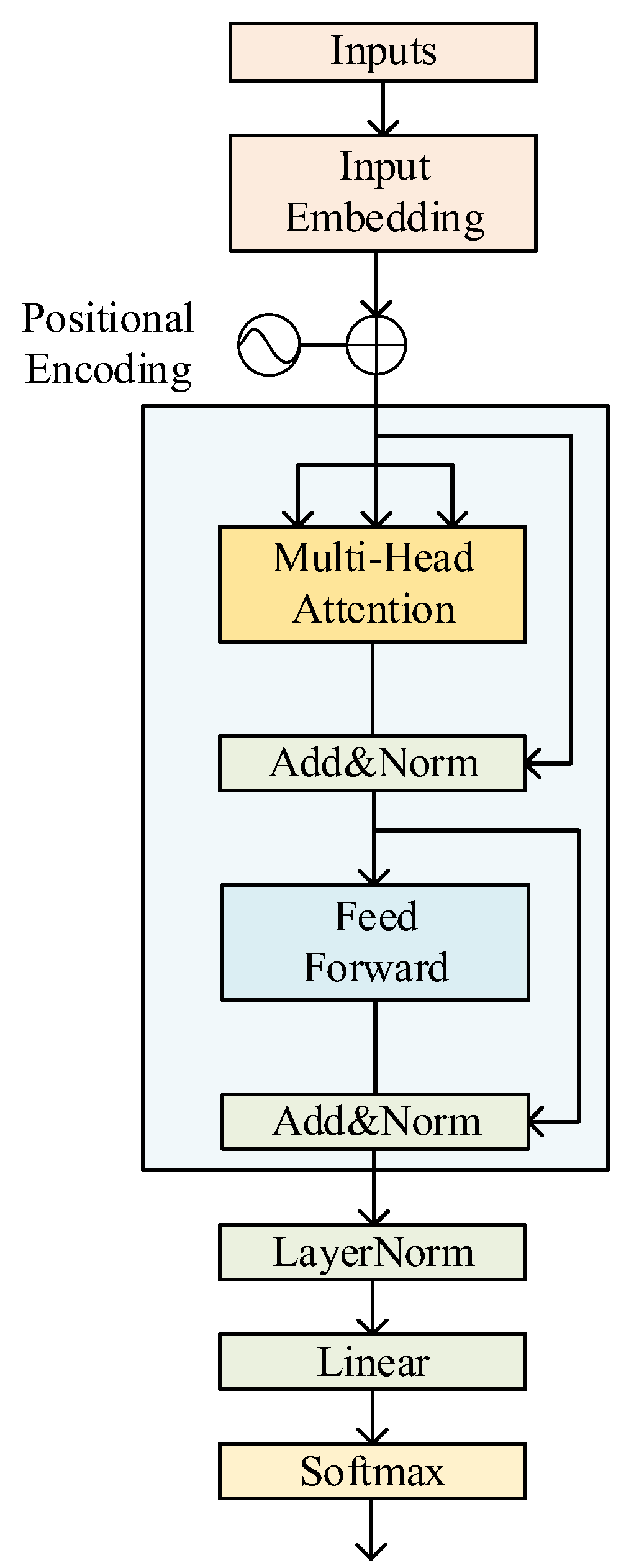
With the disjunctive graph, this paper transforms the problem by extracting useful feature information from the relationship between different nodes and sets up a feature extraction module in which a transformer is used to extract feature information [30]. This module includes a multi-head attention mechanism, position-wise feed-forward networks (FFNs), residual connection, and layer normalization (LN). The structure of the feature extraction module is shown in Figure 3. Specifically, the transformer maps all operation sequences in the input disjunctive graph to the extracted feature sequence through the self-attention mechanism, takes the embedding vector between nodes in the disjunctive graph as input, performs a self-attention calculation on the embedding vector of each node, encodes the relationship information between nodes, and calculates the product between the node embedding vector and the relational adjacency matrix.

With self-attention, the three matrices, Q (Query), K (Key), and V (Value), are all from the same input, and are computed as follows: 1. First the dot product between Q and K is calculated; with the aim to prevent the result from being too large, the value is divided by $\sqrt{d_k}$, where $d_k$ is the dimension of the Key vector and 2. The $softmax$ operation is used to normalize the result into a probability distribution and the matrix V is multiplied to obtain a representation of the sum of the weights. The calculation process is expressed as:

$$Attention\left(Q, K,V\right)=softmax(\frac{Q{K}_T}{\sqrt{d_k}})V$$

(7)

The multi-head attention mechanism further improves the self-attention layer, first mapping the Query, Key, and Value through h different linear transformations, concatenating different attentions, and finally performing a linear transformation. Each set of attention is used to map the input to a different subrepresentation space, allowing the model to focus on different locations in different subrepresentation spaces. The entire calculation process can be expressed as:

$$MultiHead\left(Q, K, V\right)=Concat({head}_1,\dots ,{head}_h)W^O$$

(8)

$${head}_i=Attention(Q{W}_i^Q,K{W}_i^K,V{W}_i^V)$$

(9)

where, $W_i^Q\in {\mathbb{R}}^{d_{model}\times d_k}$, $W_i^K\in {\mathbb{R}}^{d_{model}\times d_k}, W_i^V\in {\mathbb{R}}^{d_{model}\times d_k}$, and $W^O\in {\mathbb{R}}^{{hd}_v\times d_{model}}$ are the parameter matrices.

FFN is a fully connected feed-forward network, in which the words of each position separately pass through this exact same feed-forward neural network, consisting of two linear transformations, that is, two fully connected layers, connected by the ReLU activation function, expressed as:

$$FFN\left(x\right)=max\left(0,x{w}_1+b_1\right)w_2+b_2$$

(10)

where ${w_1,b_1,w}_2,\mathrm{a}\mathrm{n}\mathrm{d} b_2$ are trainable parameters.

Both multi-head attention and FFN use a residual connection to alleviate the problem of a disappearing gradient and then perform LN after the residual connection. The whole calculation process can be expressed as follows:

$$sub\_layer\_output=LayerNorm\left(x+SubLayer\left(x\right)\right)$$

(11)

3.4. Action Space under Data Envelopment Analysis

A single dispatching rule is limited and lacks adaptive adjustment ability. It is only applicable to a specific scenario and may not be effective in other scenarios. Therefore, this paper uses multiple dispatching rules as the action space and selects the most appropriate dispatching rule according to the current state and scheduling target. In the past, the action space composed of dispatching rules depended on the prior knowledge and parameter design experience of designers, so it was challenging to design and select appropriate dispatching rules to achieve optimization goals.

In order to solve the problem, this paper chooses data envelopment analysis [31] to select dispatching rules. Data envelopment analysis is a multi-objective decision-making method that can help decision-makers choose the most suitable dispatching rule for the current state by evaluating the performance of each dispatching rule under different objectives to minimize the makespan and maximize the machine load rate. In our study, the input of the DEA model is the predefined condition of the corresponding simulation model, which imitates the behavior of the real workshop; that is, we need to input the state characteristics of the workshop environment. Finally, each candidate scheduling rule is regarded as a separate DMU, and its production performance relative to various targets (machine load and completion time) obtained by simulation experiments is regarded as the output value of the DEA model.

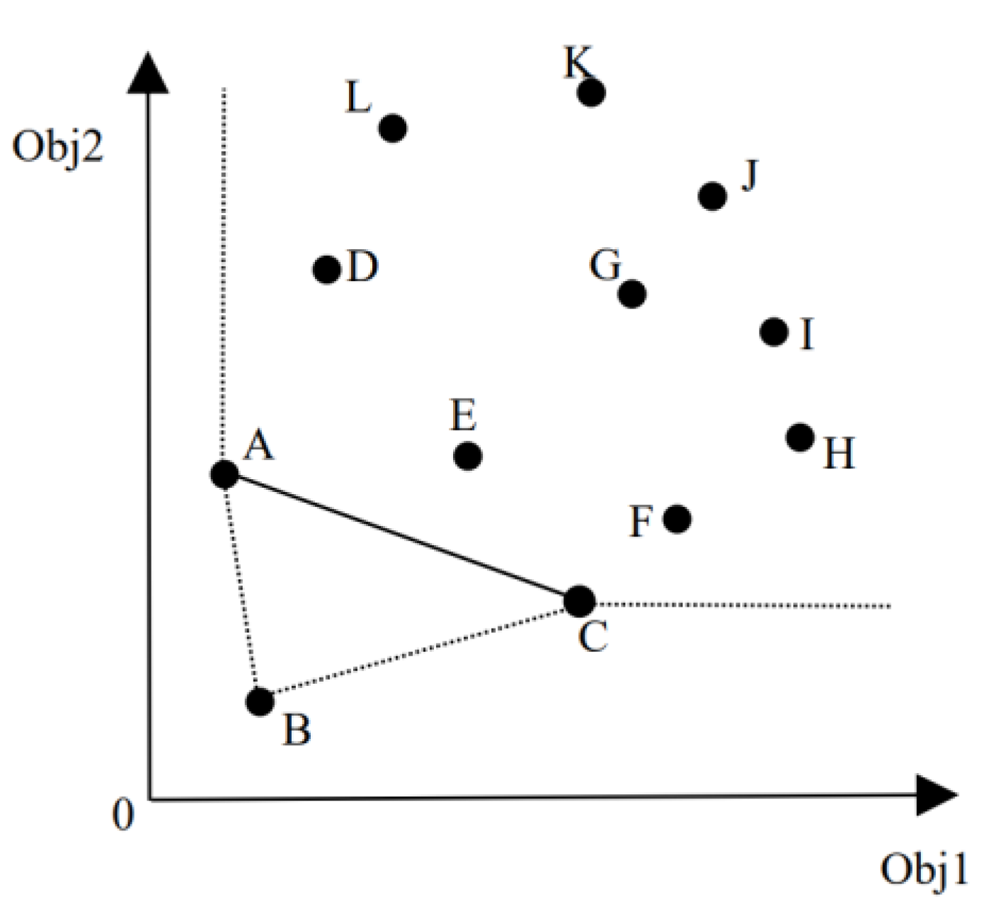
This paper selects 20 general dispatching rules. They are FIFO (first in, first out), LSO (longest processing time for the next step), LPT (longest processing time), OMCT (ordered minimum completion time), SIS (shortest total time for upcoming operation), LI (maximum imminent operation time), SRPT (shortest remaining processing time), SSO (shortest time for the next step), MOR (most remaining operations), FHALF (more than half of the total number of operations), NINQ (shortest queue), WINQ (least amount of work), LIFO (last in, first out), SJF (shortest job), WSPT (weighted shortest processing time), Random, LSPON (longest follow-up time), MS (minimum slack), WQ (work queue), and MCT (minimum completion time). Each dispatching rule defines two outputs, Obj₁ and Obj₂, the completion time and machine load related to each scheduling rule, respectively, and the strong efficiency dispatching rule and weak efficiency dispatching rule are obtained according to the efficiency score. This paper evaluated and sorted 20 general dispatching rules through data envelopment analysis and finally selected 12 optimal dispatching rules, FIFO, LSO, LPT, SRPT, SSO, MOR, FHALF, NINQ, WINQ, LIFO, LRPT, and LOR, as shown in Figure 4.

Considering the two factors of the job (operation time and number of operations) and the priority factor of the machine, this paper selected 12 dispatching rules. In order to achieve better scheduling performance, this paper also adds SPT and LSO, totaling 14 rules. They are FIFO, LIFO, LPT, SPT, LRPT, SRPT, LSO, SSO, LOR, MOR, LHALF, FHALF, NINQ, and WINQ, and their descriptions are shown in

Table 2. Definition of action space.

Dispatching Rules	Description
FIFO	First in, first out
LPT	The longer the processing time, the more priority
LRPT	Select the job with the longest remaining processing time
LSO	Select the job with the longest processing time for the next step
LOR	Select the job with the fewest remaining operations
LHALF	Select the job that has less than half of the total number of operations that have not been performed
NINQ	Select the job with the shortest queue to the next operating machine
WINQ	Select the next job with the least amount of work to operate the machine
LIFO	Last in, first out
SPT	The shorter the processing time, the more priority
SRPT	Select the job with the shortest remaining processing time
SSO	Select the job with the shortest time for the next step
MOR	Select the job with the most remaining operations
FHALF	Select the job for which more than half of the total number of operations have not yet been executed

. The design of the action space can provide more flexible and diversified scheduling strategies, which helps to improve the scheduling effect and adaptation to different application scenarios.

3.5. Reward Function

The definition of the reward function is closely related to the scheduling objective. The scheduling objective in this paper is to minimize the makespan, while the objective of the algorithm is to maximize the cumulative reward. However, in the actual production process, different scheduling problem scales are also different. In order to unify the setting of the reward function, this paper converts the long-term reward (minimizing the makespan) into an immediate reward (maximizing the machine utilization rate $U$). This transformation design improves the learning ability and decision quality of the agent. Not only can the minimization goal of the scheduling problem be transformed into the maximization goal of the cumulative reward, but the actions selected at each decision point t can also be accurately evaluated, which improves the learning ability of the agent relative to the complex control strategy.

The machine utilization rate $U$ is shown in Equation (12), which is the actual use time of the machine compared with the total available time of the equipment:

$$U=\frac{1}{M}\sum _{m=1}^M\frac{\sum _{i=1}^N\sum _{k=1}^{K_i}{E}_{ikm}}{C_{max}}=\frac{E}{M·C_{max}}$$

(12)

where $K_i$ is the total number of operations in job i, $M$ is the total number of machines, and $N$ is the total number of jobs.

Cumulative rewards are calculated as follows:

$$R=\sum _{t=1}^T{r}_t=\sum _{t=1}^{T}U\left(t+1\right)-U\left(t\right)=U\left(t\right)=\frac{E}{M·C_{max}}$$

(13)

where t is the counter, understood as the discrete-time step in reinforcement learning, $U\left(t\right)$ is the average machine utilization of time step t, and $C_{max}\left(t\right)$ is the maximum completion time of time step t.

3.6. Strategy

Traditional reinforcement learning methods usually use $\epsilon$-greedy strategies to balance exploration and exploitation [32]. Specifically, $\epsilon$-greedy strategies conduct random exploration (exploration) with the probability of $\epsilon$ and select actions with the maximum current Q value (exploitation) with the probability of 1-$\epsilon$. The method is simple and easy, but the value of $\epsilon$ needs to be adjusted manually. If the value is too large, it will lead to a lot of unnecessary exploration and reduce learning efficiency. If the value is too small, the optimal strategy cannot be explored.

In order to overcome this problem, the academic community has proposed many methods of balanced exploration and exploitation, such as the upper confidence bound (UCB) [33], Thompson sampling [34], bootstrapped DQN [35], and noisy net [36] methods. These methods are able to balance exploration and exploitation adaptively and are often more effective than traditional ε-greedy strategies.

This paper proposes a dynamic target strategy with an elite mechanism that retains some of the best-performing actions or strategies when the strategy is updated to ensure that these excellent actions or strategies will not be prematurely eliminated. By introducing the elite mechanism, reinforcement learning can strike a balance between exploration and exploitation, avoiding premature convergence and creating local optimal solutions. The strategy proposed in this paper, similar to the idea of the ε-decreasing strategy, as shown in Equations (14) and (15), relies on the scoring function $\mathcal{L}$, that is, maximizing machine utilization, and normalizing the result of the function.

$$\mathcal{L}={U\left(t\right)}_{max}=\frac{E}{M·C_{max}}$$

(14)

$$a=\left\{\begin{array}{c}\left\{\begin{array}{c}{argmax}_{a_{\prime }}Q\left(a^{\prime }\right) with probability 0.5\ast \mathcal{L}\\ {\pi }^{best}\left(s\right) with probability 0.5\ast \mathcal{L}\end{array}\right.\\ random with probability 1-\mathcal{L}\end{array}\right.$$

(15)

Over time, with more experience, the value of the scoring function will increase, gradually shifting from exploration to exploitation so as to achieve a better balance. The introduction of a dynamic target strategy can improve the stability and convergence of the reinforcement learning algorithm so that it can better cope with the needs of different environments and problems.

4. Experiments

4.1. Dataset

The OR-Library is a standard dataset widely used in the field of operations research and optimization and contains instances and descriptions of various types of problems, including scheduling, path planning, traveling salesman problems, vehicle routing problems, and other fields, for evaluating and comparing the performance of different optimization algorithms. In the field of scheduling, instances of this dataset typically include information such as the number of jobs and machines, the processing time of jobs, and so on. The advantage of the OR-Library is that it provides standardized datasets and evaluation indicators, and different researchers can use the same benchmark to compare and verify their own algorithms, ensuring the objectivity and reliability of the algorithm evaluation.

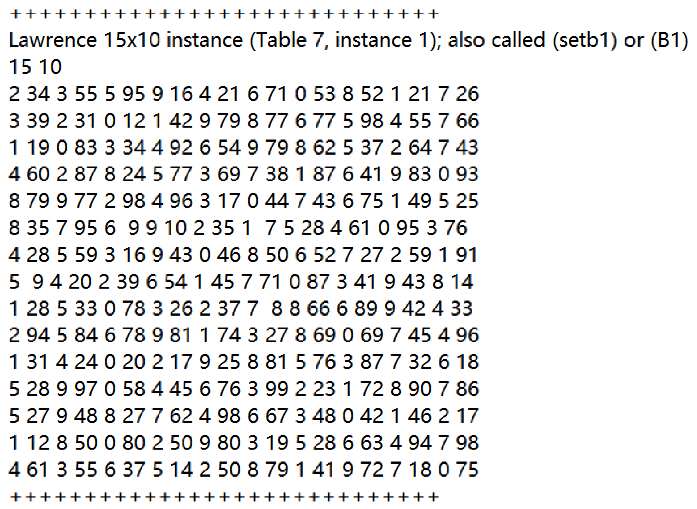
As shown in Figure 5, in the case of la21, the scale is 15 × 10, which means that there are 15 jobs and 10 machines. Taking the first line as an example, the first operation $O_{11}$ of the first job $J_1$ is performed on machine $M_2$ with a processing time of 34, the second operation $O_{12}$ is performed on machine $M_3$ with a processing time of 55, and so on. Similarly, the operations, corresponding machines, and processing times of other jobs can also be found in the description of the example. This information can help researchers and developers understand the characteristics of instances and provide a basis for the design and evaluation of scheduling algorithms.

4.2. Training Environment

This paper uses tensorflow2.0 and the neural network optimizer Adam, running on Windows 11, 64 RAM, Intel i7 2.50 GHz CPU PC platform. The dynamic interference factor is that the job arrives randomly, so the release time of the job is set randomly. The Dueling network is divided into two fully connected layers; the final hidden layer is fully connected, the value stream has one output, and the advantage stream has many outputs. In addition, batch normalization techniques are used in all convolution layers and fully connected layers except for the output layers of the two streams. In reinforcement learning, determining the value of hyperparameters is critical to the performance of the Q-network, but finding the optimal value is a challenge due to the large search space for hyperparameters. Thus, by performing a random search, this paper finds the values that produce the best performance for all instances, as shown in

Table 3. Hyperparameters.

Hyperparameter	Value
Number of episodes	8000
Schedule cycle	10
Buffer size	100,000
Discount factor γ	0.95
Target Q update frequency	200
Batch size	128
Prioritized replay α	0.6
Prioritized replay β	0.4
Number of layers of feature extraction module	3
Number of attention heads	5
Learning rate	10−5

.

4.3. Performance Evaluation

This section aims to explore the advantages of the proposed framework over traditional dispatching rules and other deep reinforcement learning methods. The framework proposed in this paper can dynamically select appropriate dispatching rules according to the environment, which is obviously more advantageous than any single scheduling rule. In addition, in order to evaluate the performance of the proposed method, it is compared with 14 single dispatching rules, the genetic algorithm (GA), and four reinforcement learning algorithms. In this paper, 14 scheduling instances in the OR-Library dataset are selected to prove the validity of the proposed method, including ft06, ft10, swv01, swv06, abz5, abz7, la01, la06, la21, la31, orb01, orb02, yn01, and yn02, which cover different scheduling problems. Compared with the traditional single scheduling rule, we can evaluate whether the framework can provide better scheduling performance in various scenarios, and prove the advantages of the framework in the learning and decision-making process compared with the genetic algorithm and four effective deep reinforcement learning methods in the scheduling field:

(1)

A total of 14 dispatching rules, including FIFO, LIFO, LPT, SPT, LRPT, SRPT, LSO, SSO, LOR, MOR, LHALF, FHALF, NINQ, and WINQ;

(2)

GA: a search algorithm that simulates the principles of natural selection and genetic inheritance. Its basic idea is to find the optimal solution to the problem by simulating the evolutionary process. The core steps of the genetic algorithm include selection, crossover, and mutation. Using the genetic algorithm to solve job-shop scheduling problem necessitates defining a coding strategy, fitness function, and genetic operation;

(3)

Advantage actor-critic (A2C): a reinforcement learning method, based on the policy gradient and value function, which is usually used to solve reinforcement learning problems in continuous-action space and high-dimensional state space. The algorithm combines an Actor network and a Critic network, generates action through the Actor network, estimates the state-value function or state-action value function through the Critic network, and finally trains the Actor network and Critic network through the strategy gradient algorithm;

(4)

Proximal policy optimization (PPO): has some advantages over the policy gradient and trust region policy optimization (TRPO). It alternates between sampling data and using the random gradient ascending method to optimize instead of the objective function. Although the standard strategy gradient method performs a gradient update for each data sample, the PPO proposes a new objective function, which can realize small-batch updates;

(5)

DQN: is one of the first widely used algorithm models for reinforcement learning in the field of deep learning. It was proposed by the research team of DeepMind in 2013 by combining deep neural networks with the classical reinforcement learning algorithm Q-learning. It realizes the processing of high-dimensional and continuous state space and has the ability to learn and plan;

(6)

Rainbow DQN: is a deep reinforcement learning method proposed by DeepMind that integrates six improvements on the basis of the DQN. Rainbow DQN combines six extended improvements to the DQN algorithm, integrating them on the same agent, including DDQN, dueling DQN, and DQN, as well as the prioritized replay, multistep learning, distributional RL, and noisy net methods.

The experimental results are shown in

Table 4. Experimental results with different dispatching rules.

Instance	Scale	Ours	Dispatching Rules
			FIFO	LIFO	LPT	SPT	LTPT	STPT	MOR	LOR	LSO	SSO	LHALF	FHALF	NINQ	WINQ
ft06	6 × 6	59	68	70	77	88	68	83	61	68	61	87	79	66	67	68
ft10	10 × 10	1052	1262	1281	1295	1074	1190	1262	1163	1352	1424	1471	1366	1253	1341	1262
swv01	20 × 10	1718	1889	2123	2145	1737	1961	1751	1971	1838	1997	2027	1989	2011	1977	1889
swv06	20 × 15	2042	2243	2331	2542	2140	2327	2360	2287	2383	2488	2452	2684	2751	2133	2243
abz5	10 × 10	1338	1388	1605	1586	1352	1483	1624	1336	1559	1725	1855	1735	1466	1564	1370
abz7	20 × 15	806	902	946	903	849	918	923	775	933	971	1101	984	951	914	900
la01	10 × 5	695	830	764	822	751	835	933	763	941	808	843	865	896	836	830
la06	15 × 5	926	1078	1031	1125	1200	1098	1012	926	1095	1011	1211	1234	1053	1134	1078
la21	15 × 10	1198	1417	1479	1451	1324	1278	1541	1251	1547	1419	1965	1763	1877	1563	1417
la31	30 × 10	1764	2148	2256	2245	1951	2083	2270	1836	2129	2147	2296	2345	1988	2238	2148
orb01	10 × 10	1163	1456	1495	1410	1478	1308	1458	1307	1410	1383	1294	1326	1671	1504	1456
orb02	10 × 10	933	1157	1264	1293	1175	1067	1166	1047	1194	1265	1347	1096	1255	1244	1157
yn01	20 × 20	1009	1158	1177	1115	1196	1177	1188	1045	1205	1314	1361	1198	1358	1146	1123
yn02	20 × 20	1074	1356	1283	1195	1256	1225	1199	1098	1446	1364	1679	1612	1421	1489	1356

and

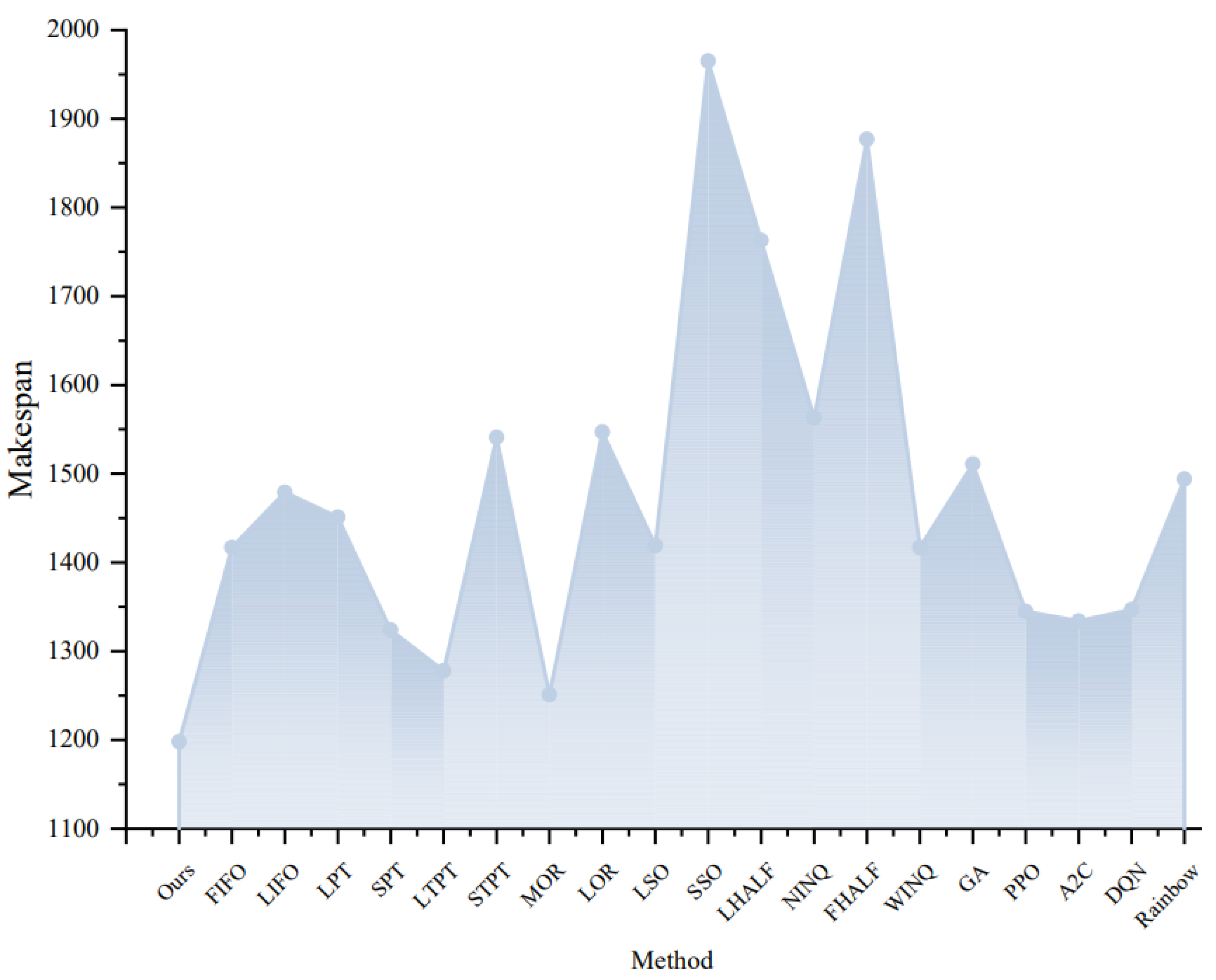
Table 5. Comparison of different algorithms.

Instance	Scale	GA	Reinforcement Learning
			PPO	A2C	DQN	Rainbow	Ours
ft06	6 × 6	59	67	69	65	63	59
ft10	10 × 10	1061	1139	1276	1223	1231	1052
swv01	20 × 10	2331	1986	1979	1962	2061	1718
swv06	20 × 15	2971	2354	2369	2311	2333	2042
abz5	10 × 10	1377	1755	1477	1635	1552	1338
abz7	20 × 15	807	985	961	897	904	806
la01	10 × 5	741	828	830	785	935	695
la06	15 × 5	994	1021	1043	984	1066	926
la21	15 × 10	1511	1345	1334	1347	1494	1198
la31	30 × 10	2443	2047	2075	1958	1846	1764
orb01	10 × 10	1463	1343	1344	1327	1473	1165
orb02	10 × 10	1010	1311	1154	1230	1098	933
yn01	20 × 20	1488	1132	1250	1109	1110	1009
yn02	20 × 20	1131	1261	1312	1455	1354	1074

. Compared with traditional dispatching rules, the method proposed in this paper has less completion time and the average performance is improved by 15.98%, which means that our method can arrange jobs and resources more effectively, thus shortening the overall completion time and improving production efficiency. Compared with the genetic algorithm, it has a smaller completion time and the average performance is improved by 17.98%, which indicates that our method has advantages in searching and optimizing scheduling strategies, and can find efficient scheduling schemes more accurately. In addition, compared to PPO, A2C, DQN, and Rainbow-based reinforcement learning, the completion time is smaller and the average performance is improved by 13.84%.

Even though Rainbow integrates six extended improvements of DQN, including DDQN, dueling DQN, prioritized replay, multistep learning, distributional RL, and noisy net, the experimental results show that the method proposed in this paper exceeds the integration of these six extended algorithms in practical effect. The ablation experiment is detailed in Section 4.4. These results validate the effectiveness of the proposed method and prove its superiority in solving scheduling problems; it can adapt to different scheduling scenarios and provide better scheduling performance in numerous cases, which means that the method has wide applicability and feasibility in practical applications, and can provide effective solutions for scheduling problems in different industries and fields.

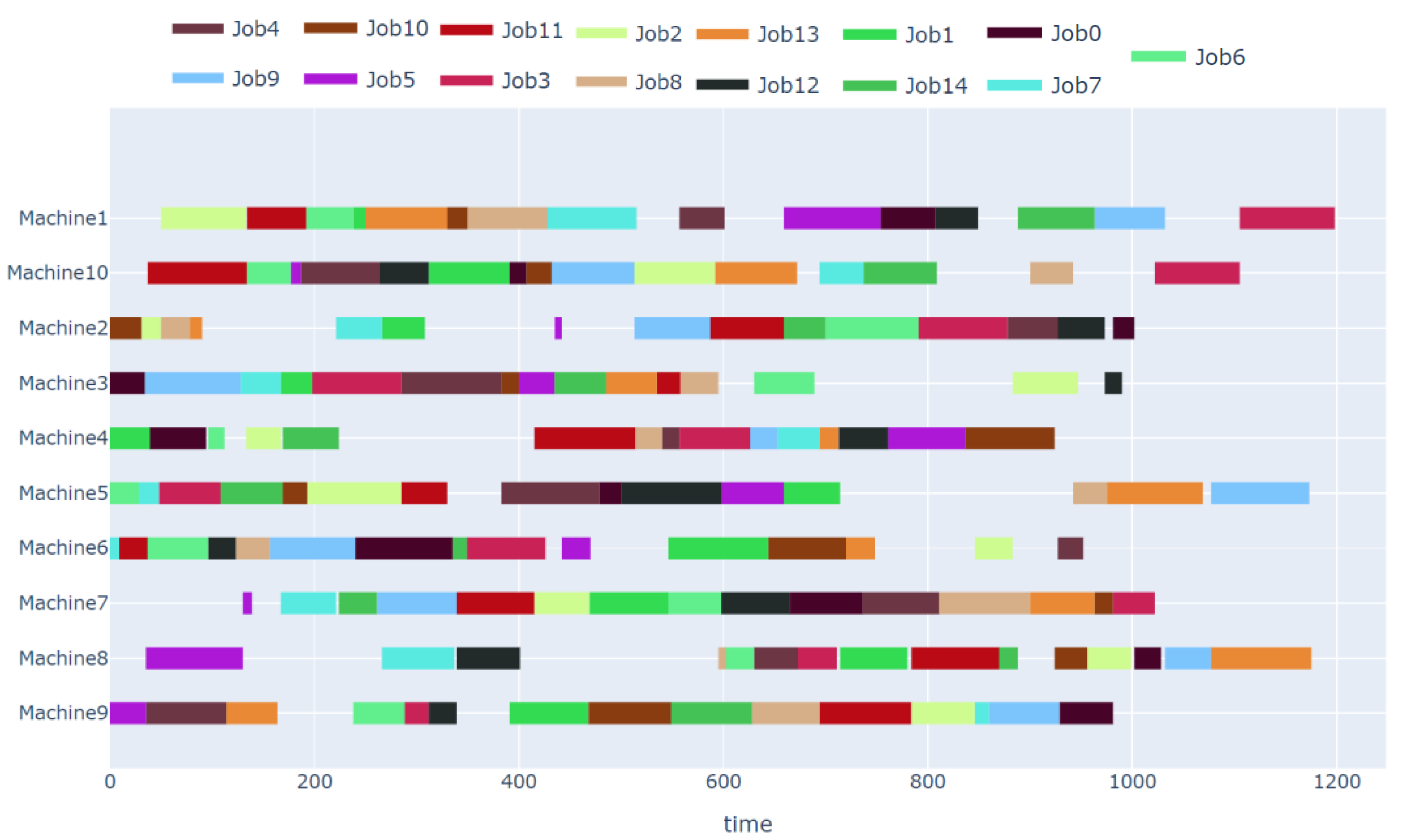
Using the framework proposed in this paper, la21 in the OR-Library dataset is taken as an example to generate a scheduling scheme. The instance scale is 15 × 10, that is, there are 15 jobs and 10 machines, and the job arrangement is shown through a Gantt chart, as shown in Figure 6. The Gantt chart shows the processing of 15 jobs on 10 machines, along with their start time and end time.

By observing the Gantt chart, it can be seen that, under the framework proposed in this paper, the makespan of this instance is 1198. Compared with other methods, the framework in this paper achieves the best scheduling performance in this instance, which can more effectively arrange the execution sequence of jobs and the utilization of resources so that all jobs can be completed in the shortest time. Through the intuitive display of the Gantt chart, we can clearly observe the arrangement of jobs, the processing time required for each job, and the utilization of machines, which has an important reference value for evaluating the effect of scheduling schemes and optimizing the scheduling process.

As shown in Figure 7, it can be seen that the framework proposed in this paper shows excellent scheduling performance on the la21 instance and minimizes the makespan through an optimal scheduling scheme, which verifies the effectiveness and feasibility of the proposed method and provides support for solving practical scheduling problems. In summary, the method proposed in this paper can improve scheduling efficiency and reduce completion time and is expected to provide reliable support for scheduling optimization in actual production and operation processes and provide valuable references for research in related fields.

4.4. Ablation Experiment

The performance evaluation experiment results in the previous section show that the performance of D3QPN is significantly better than DQN and Rainbow. Rainbow integrates six extended improvements of DQN, including DDQN, dueling DQN, prioritized replay, multistep learning, distributional RL, and noisy net. To verify the contribution of each part of the proposed method, ablation experiments were conducted in this paper, and the experimental results are shown in

Table 6. Ablation experimental results.

Instance	Makespan
	DQN	DDQN	Dueling DQN	Prioritized Replay	Multistep Learning	Distributional RL	Noisy Net	Ours
ft06	65	63	61	62	62	64	60	59
ft10	1223	1310	1307	1321	1421	1334	1294	1052
swv01	1962	1812	1785	1801	1894	1981	1794	1718
swv06	2311	2216	2177	2183	2197	2431	2274	2042
abz5	1635	1469	1397	1401	1557	1463	1576	1338
abz7	897	952	904	881	991	895	975	806
la01	785	761	752	779	757	804	743	695
la06	984	973	943	951	1064	972	958	926
la21	1347	1254	1269	1240	1367	1575	1276	1198
la31	1958	1951	1901	1876	1864	1934	1802	1764
orb01	1327	1371	1298	1366	1365	1631	1309	1165
orb02	1230	993	964	959	1074	1361	1001	933
yn01	1109	1127	1118	1123	1216	1398	1109	1009
yn02	1455	1278	1275	1307	1254	1462	1241	1074
Average	1306	1252	1225	1233	1292	1379	1244	1127

.

The results show that not all improvements on DQN in Rainbow are better than DQN itself, which indirectly indicates that not all DQN variants are suitable for DJSP; for example, distributed DQN can take less time than DQN on some events. However, it can be seen from the experimental results in the table that the overall effect is not as good as DQN. In addition, the experimental results show that distributed DQN is a negative factor used by Rainbow in DJSP. After analysis, it is found that distributed DQN adopts a distributed perspective to model the deep reinforcement learning model and selects equidistant value sampling points for decision-making, but in DJSP, there are relatively few operations to choose from. Therefore, distributed DQN has certain interference in decision-making, resulting in an increase in the completion time.

In contrast, both dueling DQN and prioritized replay are superior to DQN in the proposed method, indicating that improving these parts on DQN and using them to deal with DJSP problems has an improved effect. Through the results of ablation experiments, we can better understand the roles and contributions of each part of the proposed method and further verify its effectiveness. These experimental results provide important guidance for us to further study and improve the dynamic job-shop scheduling problem based on reinforcement learning.

4.5. Feature Extraction Evaluation

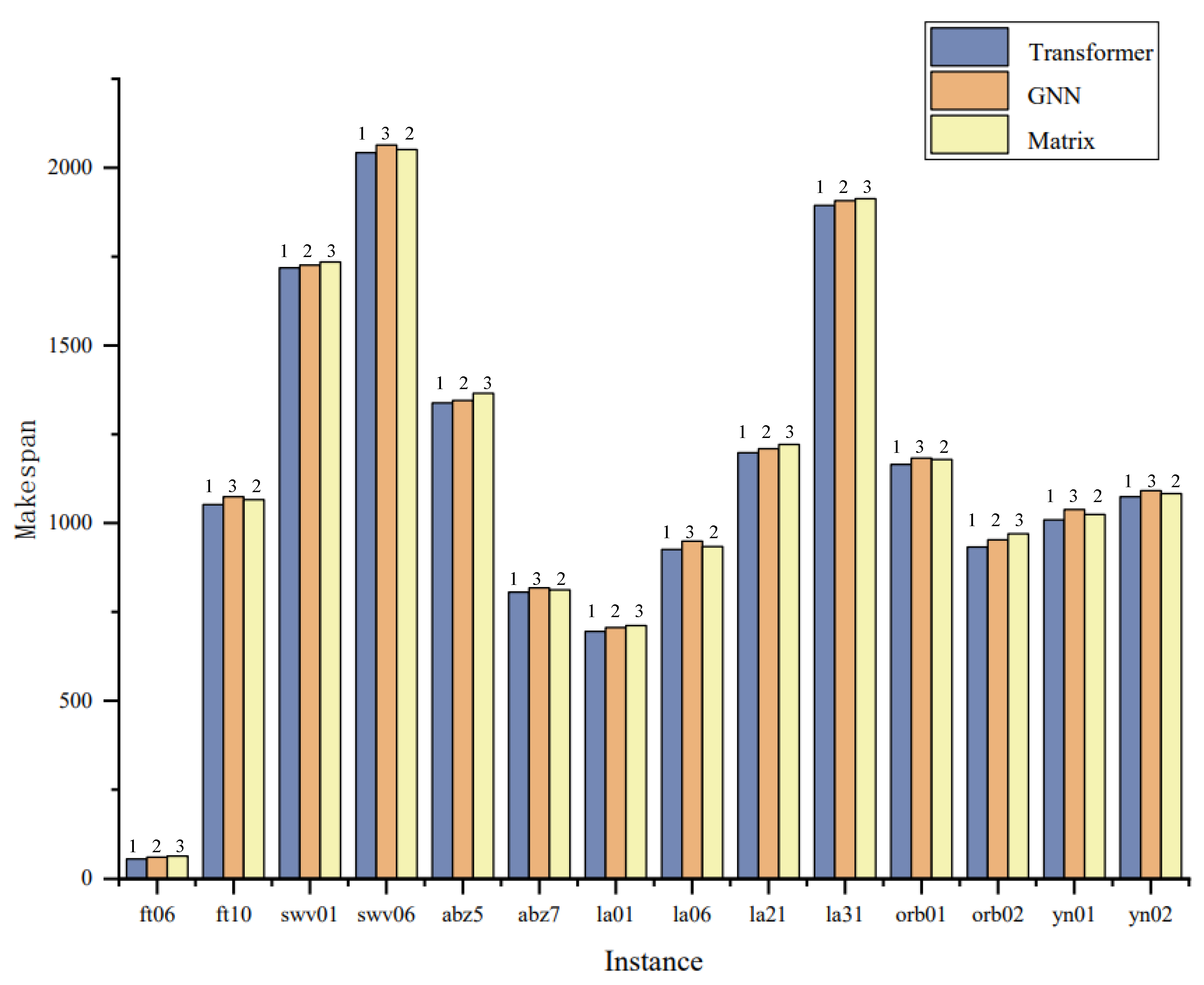
In order to verify the rationality of using a transformer as a feature extraction module, this paper conducts an experimental comparison and compares the transformer with the traditional GNN and matrix. The results are shown in Figure 8, where the ranking number indicates the relative advantages and disadvantages of each method in terms of effect. The smaller the number, the better the effect, with one indicating the highest ranking.

The experimental results show that the method of using a transformer as the feature extraction module achieves better performance in all instances, ranking the highest. The transformer can model the relationship between nodes through the self-attention mechanism, which is not only limited to the direct neighbors of nodes but also can capture the long-term dependency relationship between nodes. In contrast, GNN methods typically only consider information about local neighbor nodes and cannot capture further correlations. In addition, the attention mechanism in the transformer model can be calculated in parallel, so it has good scalability, especially when dealing with large-scale graphic data. In contrast, the GNN method and matrix representation usually require iterative updates node by node when calculating neighbor node information, which is relatively inefficient.

In the transformer’s attention mechanism, the shallow layers focus more on what is next for each job and what is not complete, ignoring what is complete; furthermore, what is complete focuses on what is complete, so you can work together to determine what each job should be doing at the moment. In summary, the experimental results clearly show the advantages of the transformer as a feature extraction module that can better capture the relationship between nodes and has good scalability and efficient computing power. The feature extraction method using a transformer has better performance and application prospects when processing graph data.

4.6. Action Space Evaluation

In the research on DJSP based on reinforcement learning, many scholars chose to dispatch rules as action space, but few demonstrated their advantages experimentally. In order to compare different action spaces, this paper selects four kinds of action spaces for comparison. The first scenario selects unconstrained operations, that is, any operation can be selected at each time step. In this case, the agent may choose any operation, including one that has already been completed, which is time-consuming and inefficient. The second scenario selects eligible operations, that is, only the operations that satisfy the constraints are selected in each time step. Although this scenario saves some time compared to the first case, it still has the problem that the efficiency is still not high. The third scenario directly selects dispatching rules as action space. By selecting the appropriate dispatching rules, the agent can make better decisions and produce a better scheduling scheme. The fourth scenario is an action space composed of dispatching rules under data envelopment analysis, which are comprehensively considered and optimized to select dispatching rules in a targeted manner, thereby greatly improving scheduling efficiency.

The experimental results are shown in

Table 7. Comparison of action space in different scenes.

Instance	Makespan
	Dispatching Rules-DEA	Candidate Dispatching Rules	Eligible Operations	Unconstrained Operations
ft06	59	68	164	5600
ft10	1052	1352	2163	9520
swv01	1718	1838	3596	27,026
swv06	2042	2383	4124	35,196
abz5	1338	1559	2764	19,650
abz7	806	933	1726	6504
la01	695	941	1367	5699
la06	926	1095	2063	7955
la21	1198	1547	2587	11,220
la31	1894	2129	3759	29,853
orb01	1165	1410	2431	13,552
orb02	933	1194	1925	8954
yn01	1009	1205	2165	9860
yn02	1074	1446	2335	10,745

; by comparing four different scenarios, the dispatching rules based on data envelopment analysis as an action space method show obvious advantages in improving scheduling efficiency. Compared with the candidate dispatching rules, the scheduling performance is improved by 17.18%. These experimental results further validate the superiority of selecting dispatching rules as action space, and, compared with unconstrained operations and eligible operations selection, the scheduling performance is improved by 91.04% and 52.97%, respectively. Selecting dispatching rules as action space not only improves the flexibility of scheduling but also improves the efficiency of scheduling, which also shows that in dynamic job-shop scheduling problems, it is very important to select the appropriate action space to improve scheduling performance. These experimental results provide a useful reference for the solution of dynamic job-shop scheduling problems in this paper and provide important guidance for the agent to choose the appropriate motion space in practical applications.

4.7. Strategy Evaluation

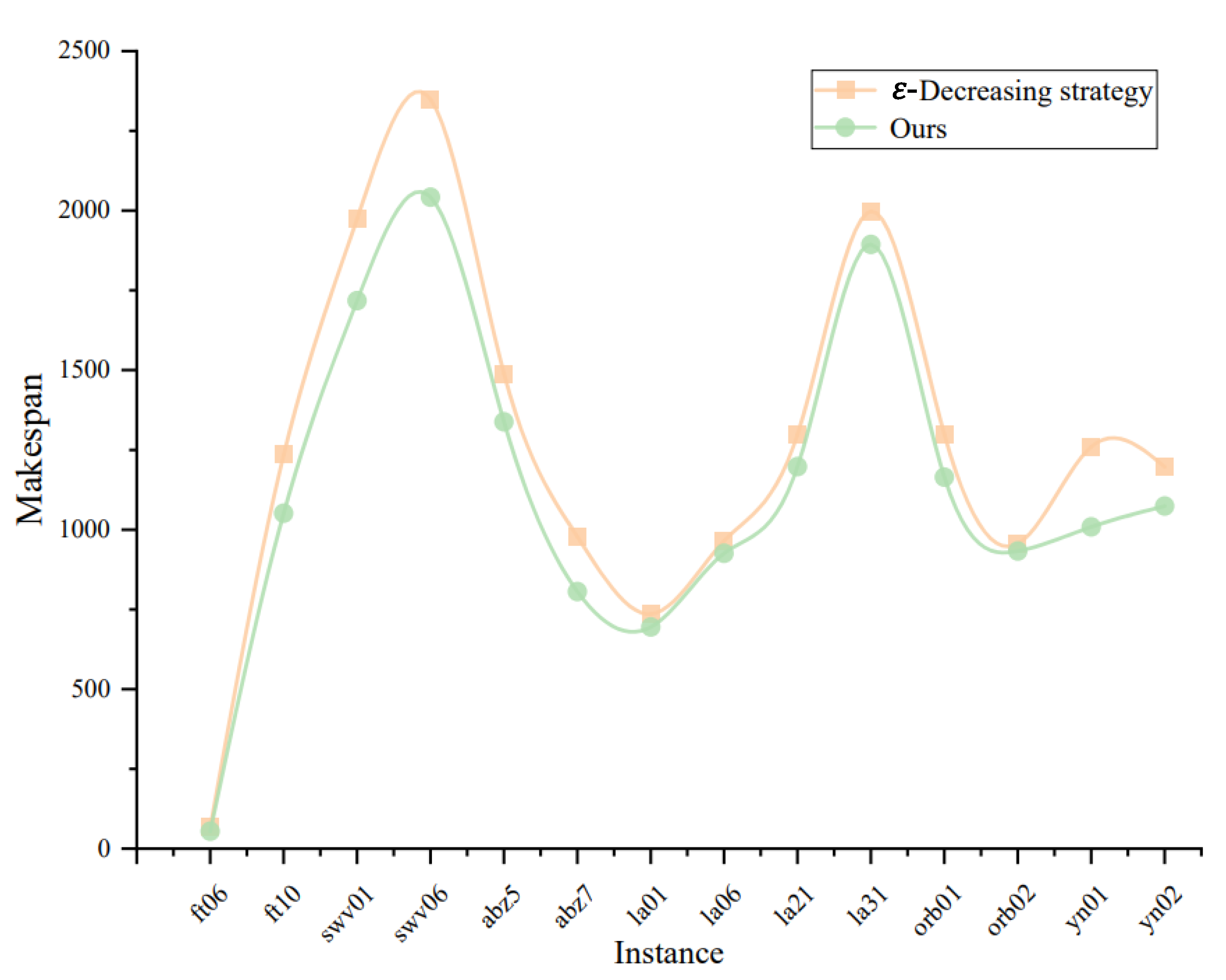
This paper also verifies the influence of the proposed dynamic target strategy with the elite mechanism on scheduling performance, as shown in Figure 9, which shows the results of two different strategies on each scheduling instance. The results show that the proposed strategy can further improve scheduling efficiency. In the later stage of training, the method using the ε-decreasing strategy is likely to choose greedy behavior, which may fall into the local optimal solution, limiting the further improvement of performance. The exploration and exploitation strategy proposed in this paper selects the global optimal solution with the same probability, which can approach the global optimal solution.

By comparing the experimental results, it can be concluded that the dynamic target strategy with the elite mechanism proposed in this paper has obvious advantages in improving scheduling performance. The implementation of this strategy enables the algorithm to explore the space more comprehensively and effectively balance the relationship between exploration and exploitation. Therefore, it can better approximate the global optimal solution, improve scheduling efficiency, and optimize the solution of job-shop scheduling problems, which further proves the effectiveness of the proposed strategy in improving scheduling performance.

5. Conclusions

This paper proposes a DJSP scheduling-problem-solving framework based on transformer and deep reinforcement learning. The framework takes the disjunctive graph as the state takes a set of scheduling rules after data envelopment analysis as action space, mapping the state to the most appropriate scheduling rules through D3QPN. It also proposes a dynamic balance exploration and exploitation strategy that verifies the effectiveness of the proposed method through a series of comparative and ablation experiments. The framework makes full use of human domain knowledge and machine computing power to achieve the goal of man–machine collaborative decision-making. In addition, the action space is divided into four scenes for comparison. The experiment shows that the scheduling rules selected by data envelopment analysis have the shortest scheduling time. In the feature extraction part, the transformer is compared with matrix representation and the GNN and the experimental results show that the transformer used in this paper ranks first in the test case. In this paper, several sets of experiments are also carried out to verify each module one by one. The experiments show that the proposed method plays a positive role in improving scheduling efficiency. In addition, the proposed strategy is compared with other strategies, proving that the scheduling performance is good. Through extensive experiments conducted on multiple examples, it was seen that our proposed framework consistently outperforms traditional dispatching rules, genetic algorithms, and other reinforcement learning methods, achieving improvements of 15.98%, 17.98%, and 13.84%, respectively.