Exploring the Mechanism of Pulse Hydraulic Fracturing in Tight Reservoirs

Abstract

Pulse hydraulic fracturing is capable of creating intricate seam networks for improved reservoir recovery, but its dynamic damage mechanism remains unclear, limiting its scientific guidance for fracturing construction. This study combined the statistical damage and viscoelastic models according to the D-P criterion and fluid flow continuity equation to establish a mathematical model of the fluid–solid coupling under pulsed hydraulic pressure. The finite element approach was used to investigate the dynamic response and damage accumulation law of tight reservoirs under various pulse parameters. The model’s correctness was verified with indoor triaxial pulse hydraulic fracturing studies, and the Changqing oilfield’s pulse hydraulic fracturing parameters were optimized. The results showed that the rock body around the borehole sustained dynamic damage when exposed to pulsed fluid pressure. The impact force increases with frequency; however, when the frequency is too high, the dynamic pore pressure cannot be stabilized. Consequently, the damage to the rock mass starts to increase and then progressively decreases with higher pulse frequencies. The ideal frequency was found to be 1 Hz. The rock body steadily accumulates damage as the number of pulses rises, increasing the damage value gradually. At the same frequency, the damage is higher for larger pulse amplitudes and ground stress differences, as well as a smaller modulus of elasticity. Pulse cycling reduces the rupture pressure by up to 26% compared to conventional hydraulic fracturing. Moreover, the Sine wave is 4–20% better than the triangle wave. The pulse damage mechanism and parameter optimization in this paper provide theoretical support for improving the effect of hydraulic fracture modification.

1. Introduction

After a 24-year decline in oil production, tight oil and gas research in North America has sparked significant progress in reservoir development [1]. The oil and gas reserves in China exceed 200 × 10⁸ t, with recoverable reserves ranging from 20 × 10⁸ t to 25 × 10⁸ t [2]. Tight reservoir fracturing and reformation primarily use horizontal well volume fracturing technology, underdeveloped natural fractures, and poor volume fracturing reformation [3,4]. Hydraulic fracturing may form a single principal fracture when the horizontal principal stress is high [5], hindering tight reservoir exploration and development. A new technology is needed to solve the above problems.

In the beneficiation of low-rank coal, dynamics simulation analyses have yielded excellent results [6,7], and scholars are gradually applying dynamics in fracturing. Pulse hydraulic fracturing effectively reduces the fracture initiation pressure during coalbed methane extraction, producing a significant fracture network near the wellbore [8,9]. Matin et al. [10] found that the stress concentration around the wellbore during pulsed hydraulic fracturing has a significant effect on fracture extension. Xi et al. [11] developed a new pulse loading method in order to accurately predict rock fractures downhole. Using 3D printing technology, Xia Y et al. [12,13] recreated columnar jointed rock bodies by sampling window technique sampling, comparing similar constants, and empirically verifying them. This opened up new avenues for research in rock engineering. Subsequently, Xia Y et al. [14] conducted true triaxial compression tests on 3D-printed specimens and compared them with the compression tests of real rocks, as well as investigated the mechanical properties of jointed rock damage [15,16], which provided a direction for rock mechanics research. Luke P. Frash et al. [17] modified granite via secondary pulsed hydraulic fracturing after conventional fracturing. The results showed a significant increase in permeability, secondary fracture development, and further extension, intersection, and formation of penetration joints in the primary fractures. This technique was more successful in enhancing the penetration than repeated conventional fracture modification. Wu et al. [18] found that the fracture development was better, and the fracture initiation pressure decreased and then increased with the pulsation frequency, and there existed an optimal frequency through pulsed hydraulic fracturing experiments. In order to obtain more complex fracture enhancement extraction [19,20], Cappa F [21] used in situ fracturing pulses to study different control flow patterns and analyze the field data with simulation. Chen et al. [22] used an experimental method to analyze the influence of fluid pressure, strain rate, pulsation amplitude, and other factors on rock damage and crack extension and found that the pulse parameters mainly influence the extension scale of microcracks. Xie et al. [23] investigated the influence law of pulsating hydraulic fracturing on the pore structure of coal; with the increase of pulsating load, the pores in the samples increased, which is more favorable to the extension of the cracks to a certain extent. Li et al. [24] showed that pulsating cycle hydraulic fracturing can reduce fracture initiation pressure by 20% compared with conventional hydraulic fracturing. Stephansson et al. [25] concluded on the basis of their experiments that the use of pulsed hydraulic fracturing reduces the breakdown pressure by almost 20 percent compared to conventional HF. Diaz et al. [26] used an experimental study to investigate the effect of different cycle time intervals on crack propagation under maximum pulsation cycling and showed that the number of cycles required for crack initiation decreases with increasing time intervals. Wu Jinjun et al. [27] analyzed the pulse fracturing feasibility in low-permeability coal seams, finding that multiple peak pressures extended the crack length and created secondary cracks during pressure relief. Zhang et al. [28] proposed pulse hydraulic injection fracturing for coal seams to create a volumetric seam network and reduce fracture initiation pressure. However, minimal studies are available regarding pulse fracturing law and frequency optimization. Nie et al. [29] developed low-frequency hydraulic pulsation fracturing technology to improve sand transport, support fractures, and reduce construction pressure. However, hydraulic pulsation can cause fatigue damage to rocks, especially at lower frequencies. He et al. [30] proposed a rectangular pulse hydraulic fracturing technique, which can be used to obtain the optimum fluid pressure in different rocks with the optimum frequency and damping coefficient. Wei et al. [31] conducted strength tests under different pulse pressures, established rock damage evolution models, and explored the laws of pulse pressure and crack extension. Anjun et al. [32] investigated the effect of cyclic loading and its parameters on coal rock fracturing and found that permeability can be increased by cyclic loading, and the lower the loading frequency, the better the fracture extension. Pulse hydraulic fracturing is a new technology that aims to reduce fracturing challenges and improve fracture modification. Although exploratory tests have been conducted, the mechanism and cumulative damage effect remain unclear.

This paper combines statistical damage and viscoelastic models to create a dynamic damage ontology model for dense rock using the D-P criterion and fluid flow continuity equation. The finite element method is used to analyze the dynamic response law of dense rock and the evolution law of pulse cycle fracturing damage and explore the fatigue damage mechanism. Based on the mechanical characteristics of the rock in tight reservoirs, pulse cycle hydraulic fracturing similarity experiments were conducted to verify the accuracy of the method, and the relevant parameters of the field wells were optimized. The pulse damage mechanism and parameter optimization in this paper provide theoretical support for improving the effect of hydraulic fracture modification.

2. The Theory of Pulse Hydraulic Fracturing Model

2.1. Dynamic Damage Intrinsic Modeling of Rocks

2.1.1. Basic Assumption

To establish an intrinsic rock damage model under the combined action of dynamic and static forces, this paper assumes the following:

• The rock sample shown in Figure 1 consists of a viscous cylinder and a damaged body with statistical and viscous characteristics.

2.

Before destruction, the material is a linear material. The mechanical properties of the material after its destruction satisfy Hooke’s law.

3.

In the case of static loading, the viscous body does not act; it only acts at a certain loading rate. It obeys the following instantonal equation:

$${\sigma }_b=\eta \frac{d\epsilon }{dt}$$

(1)

where ${\sigma }_b$ is the stress of the cohesive body and $\eta$ is the coefficient of cohesion, reflecting the cohesive properties of the rock.

4.

Assuming that the intensity of the micrometeoroid conforms to the Weibull distribution rule, its probability density function is

$$p\left(F\right)=\frac{m}{F_0}\times {\left(\frac{F}{F_0}\right)}^{m-1}\times \exp \left[1{\left(\frac{F}{F_0}\right)}^m\right]$$

(2)

2.1.2. Statistical Damage Variable

Statistical damage variables are used to characterize microdefects, microholes, and other features because of their randomness and the premise that the strength of microunits obeys statistical distribution. It is assumed that the number of failed microelements occurring in the microelements under a certain load is $N_f$ and the total number is $N$. The dynamic damage variable $D^{\prime }$ based on Weibull distribution can be obtained by substituting (2) as

$$D^{\prime }=1-\exp \left[-{\left(\frac{F}{F_0}\right)}^m\right]$$

(3)

2.1.3. Strength of the Rock Microscopic Unit

For the damage mechanism of the rock body, the Drucker–Prager damage criterion is used, and the strength of the rock microscopic unit is

$$F=f\left(\sigma \right)=\alpha I_1+\sqrt{J_2}=k$$

(4)

where $\alpha$ and $k$ are the parameters related to the cohesion c and the angle of internal friction $\varphi$ of the rock mass, $\alpha =\sin \phi /\sqrt{9+3{\sin }^2\phi }$. $I_1$ is the first invariant of the stress tensor, and $J_2$ is the second invariant of the stress bias.

In the case of triaxial static load and repeated impact, there is not only an axial static load ${\sigma }_x$ on the axis but also an impact dynamic load $\sigma$ and enclosing pressure (${\sigma }_2-{\sigma }_3$). Therefore, it is obtained as follows:

$$I_1=\frac{\left({\sigma }_x+{\sigma }_a+2{\sigma }_3\right)E\epsilon }{{\sigma }_x+{\sigma }_a-2\upsilon {\sigma }_3}$$

(5)

$$\sqrt{J_2}=\frac{\left({\sigma }_x+{\sigma }_a-{\sigma }_3\right)E\epsilon }{\sqrt{3}\left({\sigma }_x+{\sigma }_a-2\upsilon {\sigma }_3\right)}$$

(6)

2.1.4. Establishment of Damage Ontology Modeling

Taking into account a rock mass’s damage behavior under three-dimensional static loading and repetitive impacts, the relationship between the damaged and viscous bodies is expressed as $\epsilon ={\epsilon }_a={\epsilon }_b$, $\sigma ={\sigma }_a+{\sigma }_b$, where $\sigma$ is the total impact stress of the combined body in the axial direction and ${\sigma }_a$ and ${\sigma }_b$ are the impact stress suffered by the damaged and viscous bodies, respectively. The intrinsic relationships of the assemblies are as follows:

$$\sigma =E\epsilon \left(1-D^{\prime }\right)+\upsilon \left({\sigma }_y+{\sigma }_z\right)-{\sigma }_x+\eta \frac{d\epsilon }{dt}$$

(7)

The intrinsic damage relationship of the rock mass under cyclic loading established according to the Weibull distribution is

$$\sigma =E_n\epsilon \exp \left[-{\left(\frac{F}{F_0}\right)}^m\right]+\upsilon \left({\sigma }_y+{\sigma }_z\right)-{\sigma }_x+\eta \frac{d\epsilon }{dt}$$

(8)

2.2. Rock Damage Intrinsic Model

The rock damage intrinsic equation describes the changing law of the internal structure and mechanical properties of the rock. From the theory of equivalent strain assumption, it can be obtained as

$$\left[{\sigma }^{\prime }\right]=\frac{\left[\sigma \right]}{\left(1-D\right)}=\frac{\left[E\right] \left[\epsilon \right]}{\left(1-D\right)}$$

(9)

The damage intrinsic equation for sandstone specimens under hydrodynamic cycling is obtained as

$${\sigma }_1=E{\epsilon }_1\exp \left[-{\left(E{\epsilon }_1\frac{\left({\sigma }_1+{\sigma }_3\right)-\left({\sigma }_1+{\sigma }_3\right)\sin \varphi }{2F\left[{\sigma }_1-\mu \left({\sigma }_2+{\sigma }_3\right)\right]}\right)}^m\right]+\mu \left({\sigma }_2+{\sigma }_3\right)$$

(10)

The parameters F and m in the damage intrinsic model vary with the perimeter pressure, and the relationship between F, m, and the perimeter pressure can be established to obtain the damage intrinsic model under any perimeter pressure.

2.3. Rock Stress Equilibrium Equation

The total stress at a point in the rock $\sigma$ includes three components, namely the pore pressure in the wet fluid $P_w$, the average compressive stress in other nonwetting fluids $p_a$, and the effective stress $\overline{\sigma }$, which is expressed as

$$\overline{\sigma }=\sigma +(x{p}_w+(1-x)p_a)\mathit{I}$$

(11)

where $x$ is a dimensionless factor ranging from 0.0 to 1.0. The magnitude of this factor is closely related to the adhesion between the fluid and the solid.

Since $p_a\ll p_w$, the effective stress is simplified as

$$\overline{\sigma }=\sigma +x{p}_w\mathit{I}$$

(12)

Differential equilibrium equations of rock mass for deformation characteristics and stability analysis of rock mass. Based on the principle of imaginary work, the balance equation weight function is considered a variant of the true velocity $\delta v_i$, while the weight function for the boundary conditions is considered as $-\delta v_i$ and integrated over the volume of the microelement, resulting in

$${\displaystyle {\int }_V\left({\sigma }_{ij,j}+f{}_i\right)}\delta v_i\mathrm{d}V-{\displaystyle {\int }_{S_a}\left({\sigma }_{ij}{n}_j-t_i\right)}\delta v_i\mathrm{d}S=0$$

(13)

The effective stress matrix is expressed as

$$\overline{\mathit{\sigma }}=\mathit{\sigma }+p_w\mathit{m}$$

(14)

where $p_w$ is pore fluid pressure, Pa $\mathit{m}={\left[1,1,1,0,0,0\right]}^T$.

When relating this to the intrinsic equation of the material, the matrix expression for the equivalent force is obtained as follows:

$$\overline{\mathit{\sigma }}=\mathit{D}\overline{\mathit{\epsilon }}+{\overline{\mathit{\sigma }}}^0=\mathit{D}\left(\mathit{\epsilon }+\frac{p_w-p_w^0}{3K_g}\mathit{m}\right)+{\overline{\mathit{\sigma }}}^0=\mathit{D}\mathit{\epsilon }+\frac{\mathit{D}\mathit{m}}{3K_g}{p}_w-\frac{\mathit{D}\mathit{m}}{3K_g}{p}_w^0+{\overline{\mathit{\sigma }}}^0$$

(15)

When the surface and volume force vectors are considered conservative force loads, and the large deformation effect is taken into account, then

$${\displaystyle {\int }_V\left[\frac{1}{J}{\mathit{B}}^{\mathrm{T}}\mathrm{d}\left(J\mathit{\sigma }\right)+\left(\mathrm{d}{\mathit{B}}^{\mathrm{T}}\right)\mathit{\sigma }\right]}\mathrm{d}V={\displaystyle {\int }_{S_{\sigma }}{\mathit{N}}^{\mathrm{T}}\mathrm{d}}\mathit{t}\mathrm{d}S+{\displaystyle {\int }_V{\mathit{N}}^{\mathrm{T}}\mathrm{d}\mathit{f}}\mathrm{d}V$$

(16)

2.4. Fluid Seepage Equilibrium Equation

The fluid’s flow through a porous material at different pressures and temperatures, as well as the relationship that results between pressure and flow, are described by the equilibrium equation for fluid percolation. When the surface area of the rock is $S$, and the volume of its microelement is $V$, then the mass change rate of the wet liquid within the volume $V$ is

$$\frac{\mathrm{d}}{\mathrm{d}t}{\displaystyle {\int }_V{\rho }_w{n}_w\mathrm{d}V}={\displaystyle {\int }_v\frac{1}{J}}\frac{\mathrm{d}}{\mathrm{d}t}\left(J{\rho }_w{n}_w\right)\mathrm{d}V$$

(17)

where $n_w$ is the porosity and ${\rho }_w$ is the wet liquid density, kg/m³.

The mass of the wet liquid per flow into the microscopic cell body is

$$-{\displaystyle {\int }_S{\rho }_w{n}_w{\mathit{n}}^{\mathrm{T}}}\cdot v_w\mathrm{d}S$$

(18)

where ${\mathit{n}}^T$ is the outer normal vector of the surface $S$ and $v_w$ is the seepage velocity, m/s.

According to the mass conservation law, when the mass of the liquid entering the micrometeoroid via the surface is equal to the increase in its own mass. The fluid flow momentum equation is

$${\mathit{v}}_w=-\frac{1}{n_{w}g{\rho }_w}\mathit{k}\cdot \left(\frac{\partial p_w}{\partial \mathit{x}}-{\rho }_w\mathit{g}\right)$$

(19)

where $\mathit{k}$ is the permeability coefficient vector, unfactored, and $\mathit{g}$ is the gravitational acceleration vector, m/s².

2.5. Cumulative Evolution of Cyclic Load Damage

Rocks with lower load levels and higher strengths will generally have comparatively longer fatigue lifetimes. The S-N curve yields the top stress limit, which is as follows:

$$\log (S-S_{f1})=A-B\log N$$

(20)

where A, B are coefficients to be determined by the nature of the material.

The effect of load frequency on fatigue life is

$$S=C{N}^{-A}(1+B\log N_f)C_f$$

(21)

where $C_f=1+a\left(1-bR\right)\log f$, A, B, C, a and b are relevant to the experiment.

Since the material’s stiffness gradually diminishes with reciprocating loads, it is important to average the strain magnitude under each reciprocating load. To account for the impact of load frequency on stress level, a correction factor $\eta$ is added.

$$\eta =\frac{{\sigma }_d}{{\sigma }_c}=C_1+C_2^{}\log f$$

(22)

Then, the corrected upper limit stress ratio is given by

$$S^{\prime }=\frac{{\sigma }_{\max }}{{\sigma }_d}=\frac{{\sigma }_{\max }}{M_{\mathrm{r}}\cdot {\sigma }_c}=\frac{S}{M_{\mathrm{r}}}$$

(23)

3. Examining the Pulse Parameter Influence Law

3.1. Cohesive Force Model

As shown in Figure 2, the ABAQUS cohesive element follows the traction separation criterion when the normal-phase cohesive element surface stress is below $t_n$; the stress is proportional to the displacement, and the stress reaches $t_n$, the cohesive element is damaged, and the stress it can withstand gradually decreases with an increase in displacement. When the displacement reaches $d_n$, its strength declines to zero, and the cohesive element is considered completely damaged.

The two tangential directions display the same damage pattern. Cohesive elements exhibit linear elasticity when the normal displacement is below the initial damage displacement $d_n^0$, softening when the stress reaches the tensile strength $t_n^0$ of the material. When the complete damage displacement reaches normal damage displacement, and the tensile stress is 0, the cohesive elements crack, which is expressed as

$$\max \{\frac{t_n}{t_n^0},\frac{t_s}{t_s^0},\frac{t_t}{t_t^0}\}=1$$

(24)

where $t_n^0$ is the critical stress normal to the cohesive elements, representing the tensile strength of the rock, and $t_s^0$ and $t_t^0$ are the critical stresses in the first all-direction and the second tangential direction, respectively.

The cohesive cell expansion criterion uses stiffness degradation to describe the cell damage evolution process and is generally expressed as

$$\{\begin{array}{c}{t}_s=\left(1-D\right)\overline{t_s}\\ t_n=\{\begin{array}{c}\left(1-D\right)\overline{t_n}\\ \overline{t_n}\end{array}\\ t_t=\left(1-D\right)\overline{t_t}\end{array}$$

(25)

where $\overline{t_n}$, $\overline{t_s}$, and $\overline{t_t}$ are the stresses predicted in the normal direction, the first all-direction, and the second tangential direction, respectively, of the cohesive cell at the current strain according to the undamaged linear elastic traction–separation criterion. $t_n$, $t_s$, and $t_t$ are the actual stresses in the three corresponding directions.

The damage factor of the linear stiffness degradation criterion is calculated as

$$D=\frac{d_m^f\left(d_m^{max}-d_m^0\right)}{d_m^{max}\left(d_m^f-d_m^0\right)}$$

(26)

where $d_m^{\mathit{max}}$ is the maximum displacement amplitude reached by the unit during loading, $d_m^f$ is the displacement amplitude when the unit is completely damaged, and $d_m^0$ is the displacement amplitude of the unit at the time of initial damage.

When multiple types of damage are generated in the cohesive elements, the equivalent displacement is introduced:

$$d_m=\sqrt{d_n{}^2+d_s^2+d_t^2}$$

(27)

The damage factor, also known as the exponential stiffness degradation, is expressed as

$$D=1-\left\{\frac{d_m^0}{d_m^{max}}\right\}\left\{1-\frac{1-exp\left(-\alpha \left(\frac{d_m^{max}-d_m^0}{d_m^f-d_m^0}\right)\right)}{1-exp\left(-\alpha \right)}\right\}$$

(28)

where $\alpha$ is an index describing the rate of crack expansion, and $\alpha$ defines the magnitude of the rate at which the curve decreases.

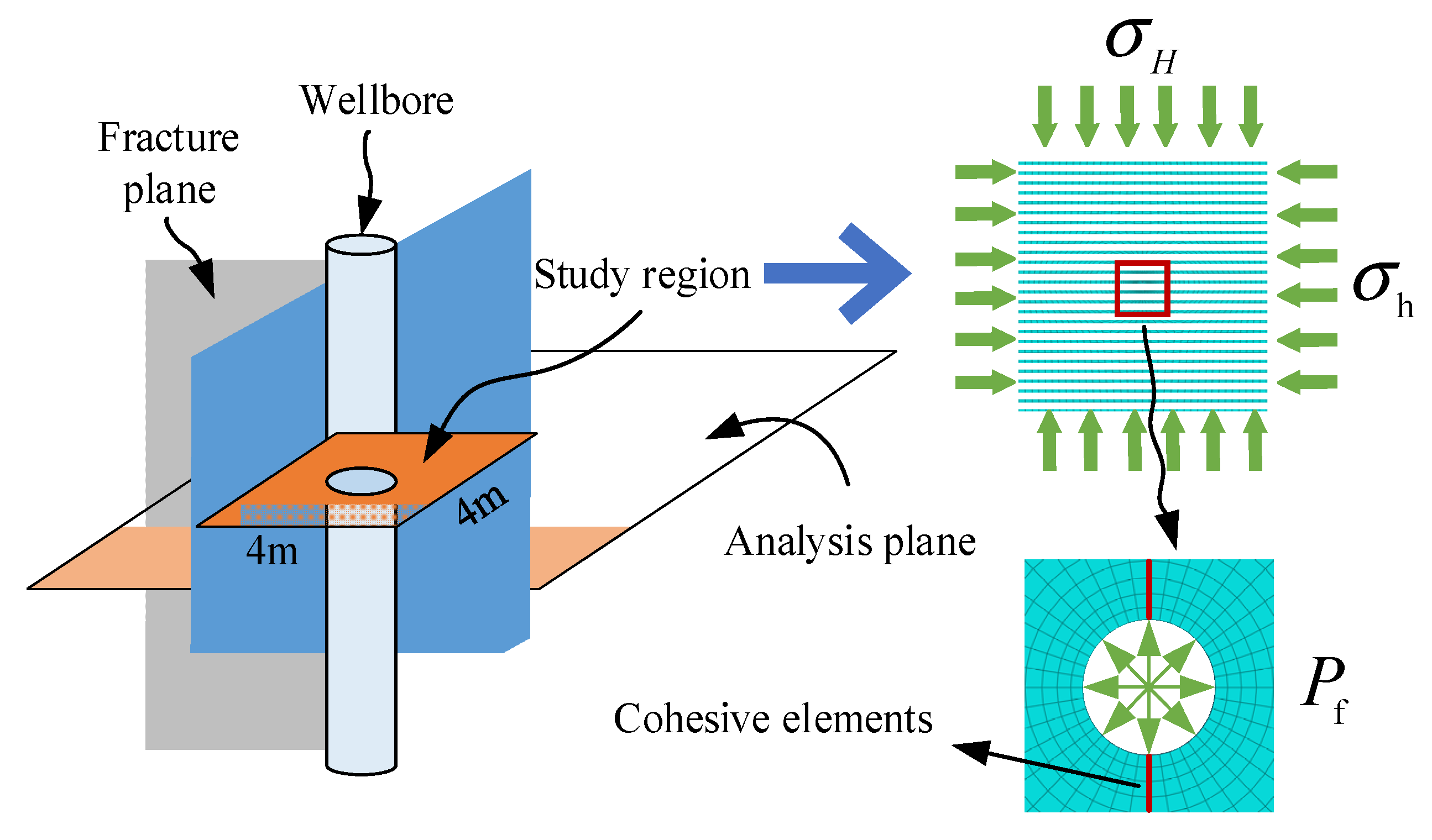
3.2. The Finite Element Modelling of Circular Hydraulic Fracturing

The simulation analysis shown in Figure 3 used 2436 cpe4p units for formation and 88 coh2d4p units for cracks. Displacement constraints, impermeable boundaries, horizontal maximum and minimum principal stresses, and pulsed cyclic water pressure were applied to the shot hole eye section of the specimen.

The rock material parameters were simulated using a finite element model used for cyclic load impact experiments by previous studies [33], as shown in

Table 1. The rock dynamic material parameters.

Number of Impacts	Dynamic Strength/MPa	Modulus of Elasticity/GPa
1	55	50
2	50	46
3	40	39
4	35	31

.

Studies [34] have shown that the strength of the rock in dynamic conditions displays a power function relationship with the loading rate. The strain rate during the pulse cycle simulation was extracted by the subroutine, while the cohesive material parameters during the pulse cycle simulation were controlled according to the relationship between the strength of the rock and the strain rate.

Table 2. The simulation comparison program design.

Groups	Pulse Frequency/Hz	Differential Ground Stress/MPa	Modulus of Elasticity/GPa	Maximum Stress/Mpa	Variant
A	1	4	28	40	——
B	0.1–10	4	28	40	Frequency
C	1	0–12	28	40	Differential ground stress
D	1	4	22–46	40	Modulus of elasticity
E	1	4	28	37–42	Maximum stress

shows the specifically designed comparison programs.

Group A represented the control group, while the B, C, D, and E variables denoted the frequency, ground stress difference, modulus of elasticity, and maximum stress. These groups were loaded with sinusoidal and triangular pulse waveforms in order to study the laws of waveform influence on pulsed hydraulic fracturing.

3.3. The Dynamic Response Law of Dense Rock Exposed to Different Impulse Parameters

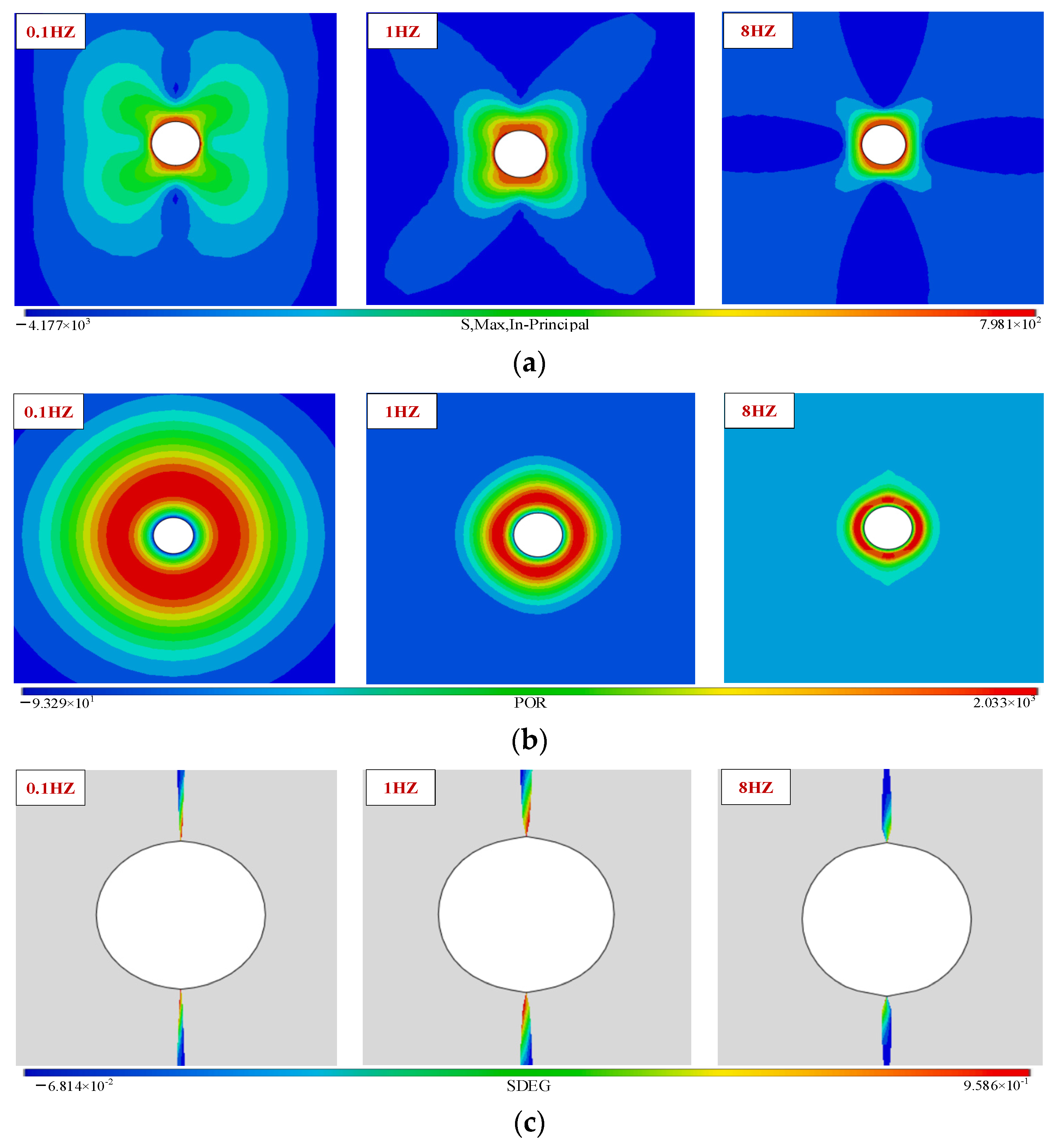
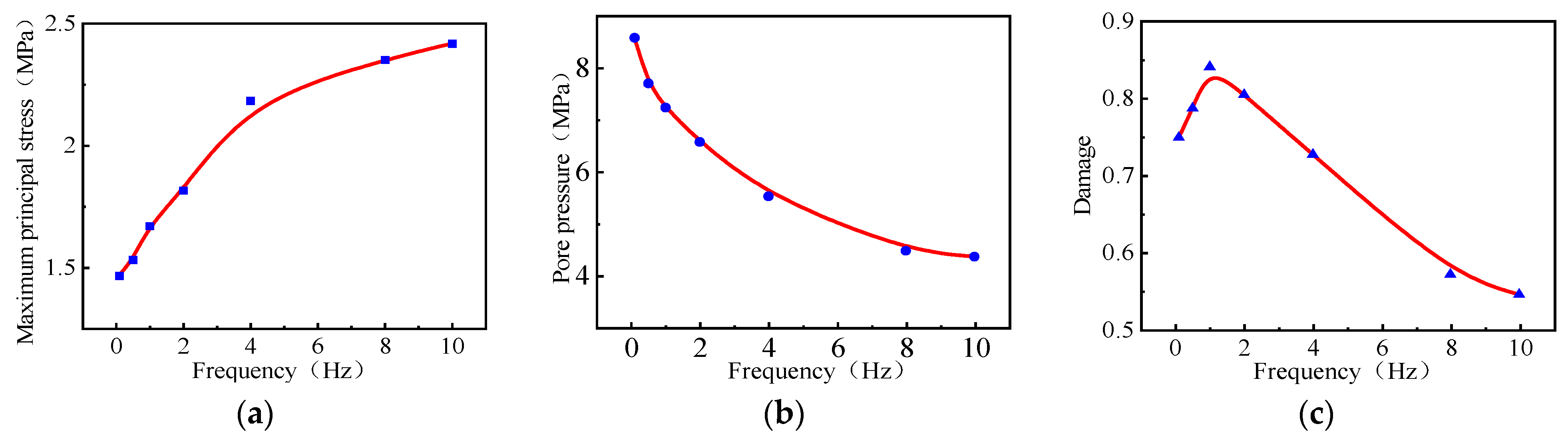
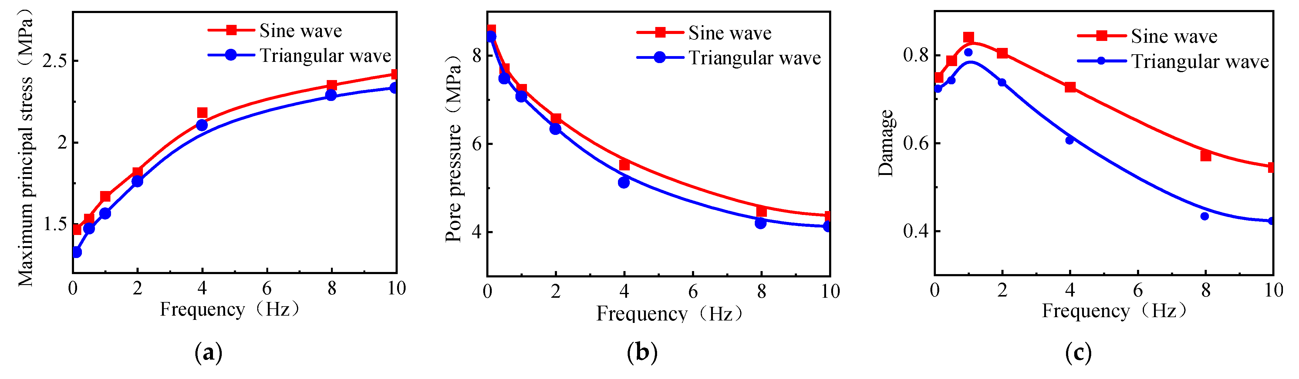
3.3.1. Pulse Loading Frequency

Compared and contrasted are the two groups, A and B, thus studying the effect of frequency on pulsed hydraulic fracturing. Pulsed water pressure was applied in a 0.1 Hz–10 Hz frequency range, while the maximum principal stress cloud, pore pressure cloud, damage cloud, and influence law curves of the plane around the borehole were extracted, as shown in Figure 4 and Figure 5. The maximum principal stress around the borehole increased with the pulse water pressure frequency since higher frequencies increased the mechanical properties and dynamic response. At higher frequencies, due to the presence of hydraulic osmosis, the pore pressure is too late to diffuse in a short period of time, the stabilized dynamic pore pressure value decreases, and the range of diffusion of the pore pressure cloud and value decreases with the increase of frequency. The maximum damage value around the borehole showed an initial increase, followed by a decline, reaching a maximum of 1 Hz. The combined effect of the maximum principal stress and pore pressure was analyzed, indicating 1 Hz as the optimal pulse frequency for the damage response at different pulse frequencies.

3.3.2. Differential Ground Stress

Compared and contrasted were the two groups, A and C, thus studying the effect of differential ground stress on pulsed hydraulic fracturing. The principal stress, pore pressure, damage, and influence law curves at a 1 Hz pulse frequency are displayed in Figure 6 and Figure 7, at ground stress values varying from 0 MPa to 12 MPa. As the geostress difference increased, the principal stress and damage value in the borehole plane gradually rose while the model pore pressure remained almost unchanged. The ground stress difference minimally affected the model pore pressure.

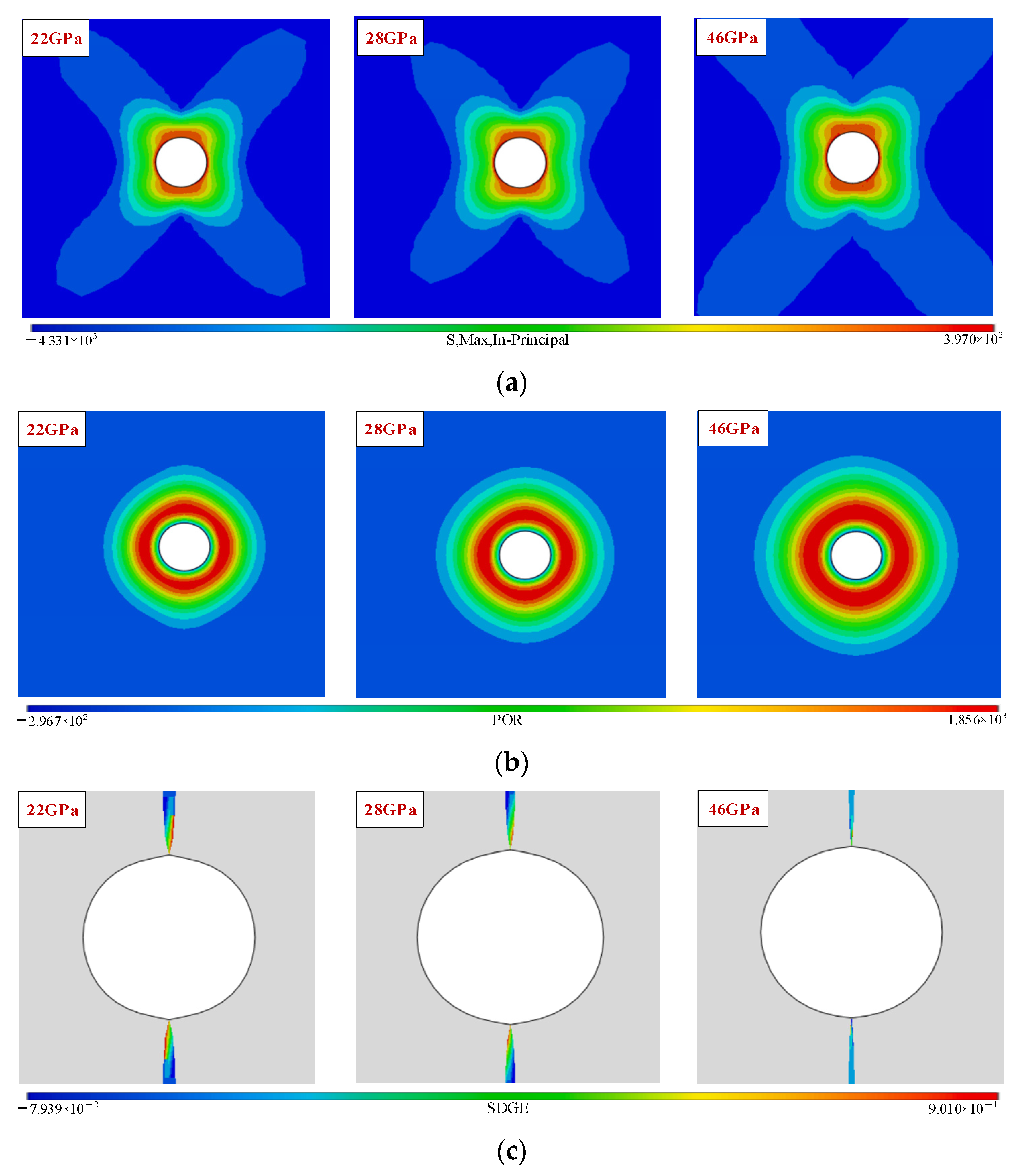
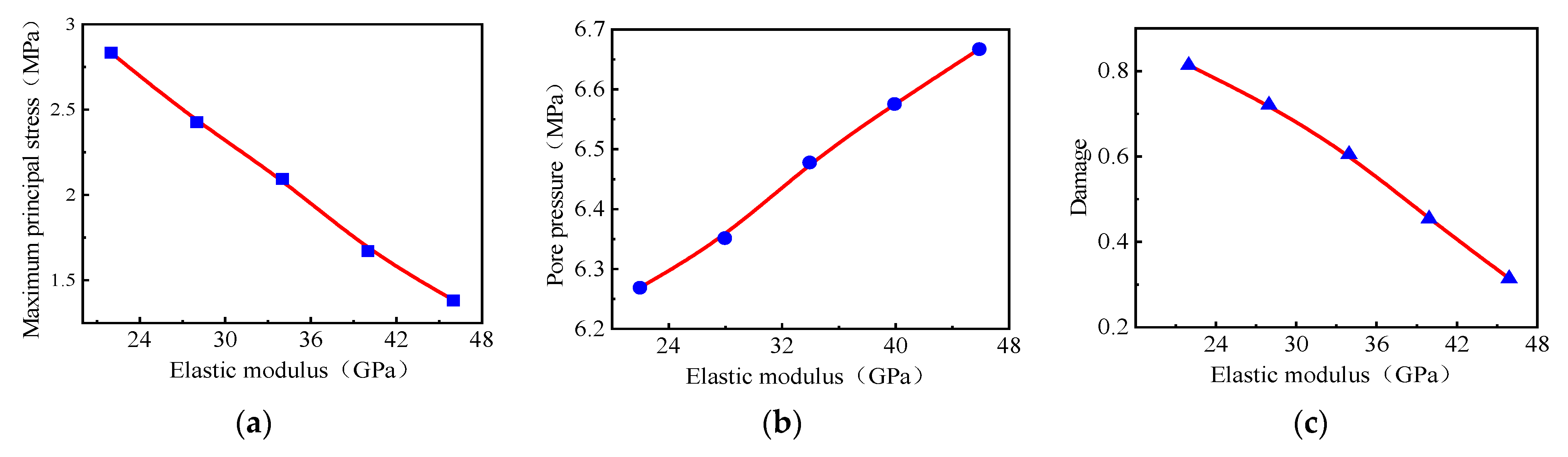
3.3.3. Modulus of Elasticity

Compared and contrasted were the two groups, A and D, thus studying the effect of modulus of elasticity on pulsed hydraulic fracturing. The maximum principal stress, pore pressure, damage, and influence law curves in the plane with elastic moduli ranging from 22 GPa to 46 GPa at a 1 Hz pulse frequency are shown in Figure 8 and Figure 9. The maximum principal stress in the borehole plane decreased as the modulus of elasticity and formation strength increased. This reduced the maximum principal stress, increased the pore pressure, and decreased the damage.

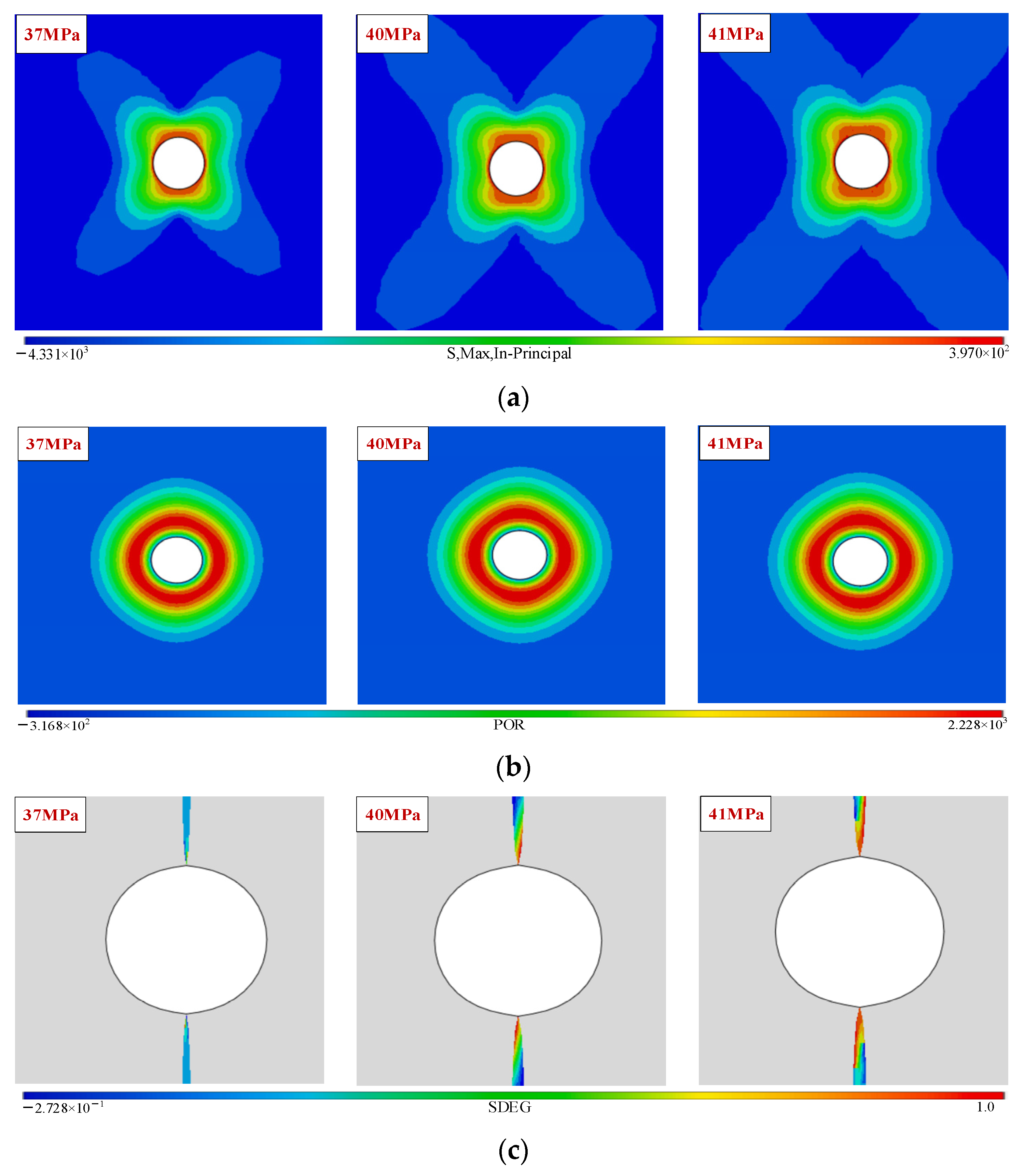
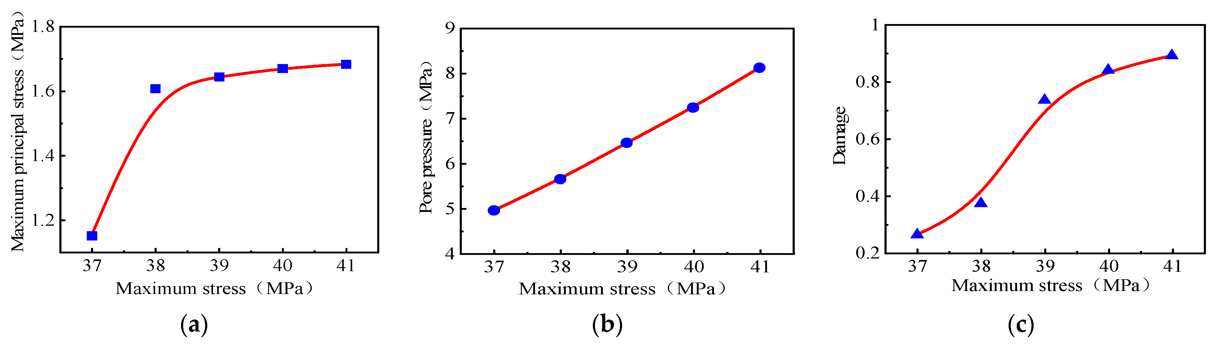
3.3.4. Maximum Stress

Compared and contrasted were the two groups, A and E, thus studying the effect of Maximum stress on pulsed hydraulic fracturing. The maximum principal stress cloud, pore pressure cloud, damage cloud, and influence law curves of the plane at a 1 Hz pulse frequency and 37 MPa–41 MPa maximum stress are shown in Figure 10 and Figure 11. At higher maximum stress, the principal stress in the eyelet plane, range of action, damage, and pore pressure around the eyelet gradually increased. This increased the pressure and reduced the pore space, leading to higher pore pressure. The dynamic response remained constant due to load action, with little effect on diffusion.

3.3.5. Pulse Waveforms

The model was simulated using triangular and sinusoidal waves to obtain the maximum principal stress, pore pressure, and damage influence law curves around the eyelet, as shown in Figure 12, Figure 13 and Figure 14. Under the same circumstances, the pressurization effect of different pulse waveforms and the decay rate of the pressure wave with the propagation distance are different, and when the pulse frequency is changed, the change of pressurization effect of different waveforms is also different. Higher pore pressures during hydraulic fracturing are prone to damage and then fracture initiation, and the higher the damage value, the more likely the fracture initiation will occur. The magnitude of the value is calculated by comparing the damage value. Comparative damage value analysis showed that the sinusoidal waveforms presented a 4–20% better effect than the triangular waveforms.

4. Study of Damage Accumulation Cracking Mechanism

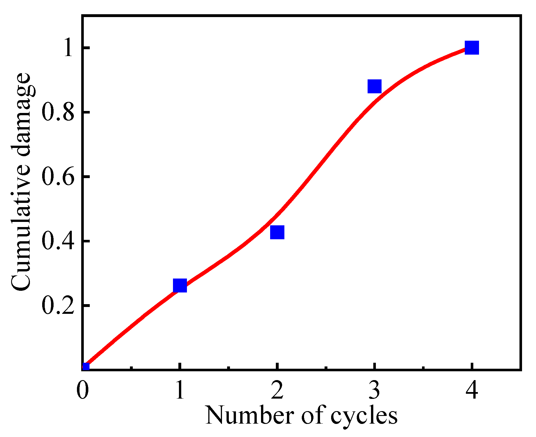
4.1. Cyclic Cumulative Damage Theory

The Corten–Dolan [35] model uses a nonlinear fatigue cumulative damage theory to assume multiple damage kernels on the surface of a specimen due to stress levels. The damage is assumed to be $D=mr{n}^a$ after n actions under equal amplitude loading, where m is the number of damage nuclei, r is the crack expansion coefficient positively correlated with the stress level, and $a$ is a constant. When the test specimens are subjected to ${\sigma }_1$ and ${\sigma }_2$ stress levels, the fatigue life of $n_1$ and $n_2$ are destroyed, and the total damage is $D_t$, then, when the ${\sigma }_1$ and ${\sigma }_2$ stress levels (assuming ${\sigma }_1$ > ${\sigma }_2$) act alternately on the specimen, the number of damage nuclei $m_1=m_2$ and $a$ represent the same constant. Based on the above assumptions, if the total number of cycles for the two stress levels is $N_f$ and the proportion of ${\sigma }_1$ and ${\sigma }_2$ during the entire process is ${\lambda }_1$ and (1 − ${\lambda }_1$), respectively, then

$$\frac{N_f}{n_1}=\frac{1}{{\lambda }_1+{\left(r_1/r_2\right)}^{\frac{1}{a}}\left(1-{\lambda }_1\right)}$$

(29)

where ${\left(r_1/r_2\right)}^{\frac{1}{a}}$ is related to the stress ratio:

$${\left(r_1/r_2\right)}^{\frac{1}{a}}={\left({\sigma }_1/{\sigma }_2\right)}^d$$

(30)

where d is a constant and can be obtained experimentally. Extension to the Corten–Dolan model with multilevel load effects is

$$\frac{N_f}{n_1}={{\displaystyle \sum }}_{i=1}^k\frac{1}{{\left({\sigma }_1/{\sigma }_2\right)}^d{\lambda }_1}$$

(31)

Xie et al. [36] improved the modulus of elasticity method, defining the elastic-plastic damage influenced by irreversible plastic deformation under one-dimensional conditions and considering the elastic-plastic and viscous material damage characteristics:

$$D=1-\frac{\epsilon -{\epsilon }^{\prime }}{\epsilon }\frac{E^{\prime }}{E}$$

(32)

where $E^{\prime }$ is the unloaded modulus of elasticity of the elastoplastically damaged materials, and ${\epsilon }^{\prime }$ is the residual plastic deformation after unloading.

Figure 15 shows a simulation flow chart of the cumulative effect of rock damage under a pulse cycle load, allowing material parameters to change as the number of pulse cycles increases.

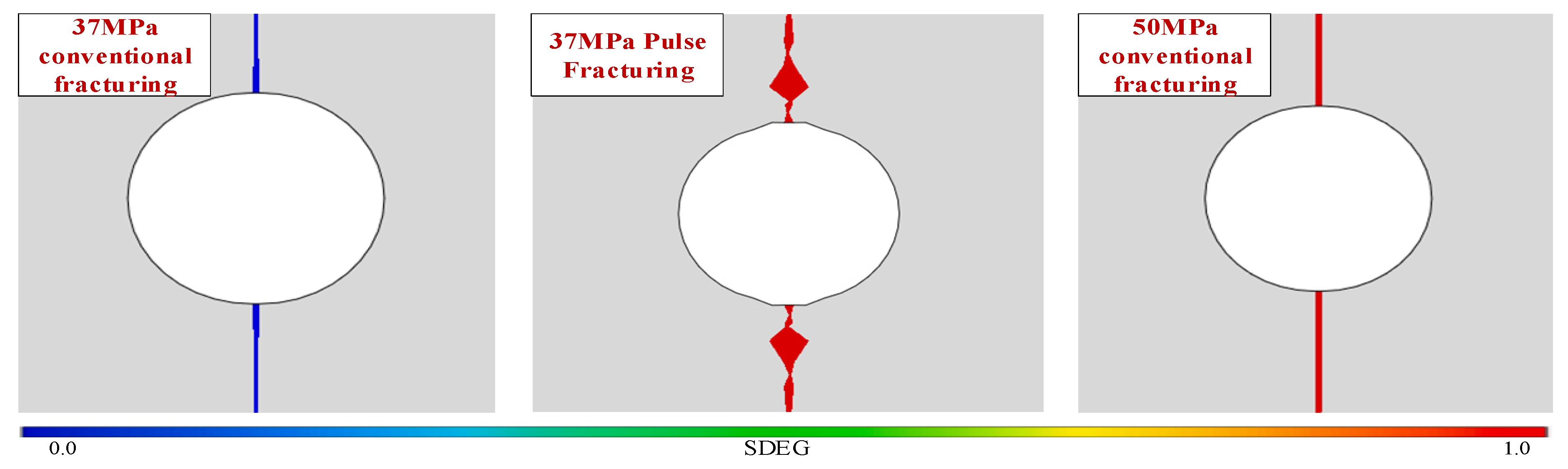
4.2. The Effect of Static and Dynamic Loading Methods on Rupture Pressure

Cyclic loading during hydraulic fracturing can cause fatigue damage that reduces model strength. To compare the performance of pulse hydraulic fracturing with conventional hydraulic fracturing, pulse fracturing with a load of 37 MPa and conventional fracturing with a load of 50 MPa were calculated separately. Figure 16 shows the damage cloud diagrams, while Figure 17 presents the cumulative damage curve.

The comparison showed that conventional hydraulic fracturing did not cause damage under the same load, while damage was evident when exposed to pulsed hydraulic fracturing. The damage to the model at an impulse load of 37 MPa reached 1 after four cycles, causing complete destruction. Pulsed hydraulic fracturing damaged the rock at lower pressures, reducing the rupture pressure from 50 MPa to 37 MPa, representing a 26% decrease.

4.3. Effect of Different Impulse Parameters on the Damage Cumulative Damage Law

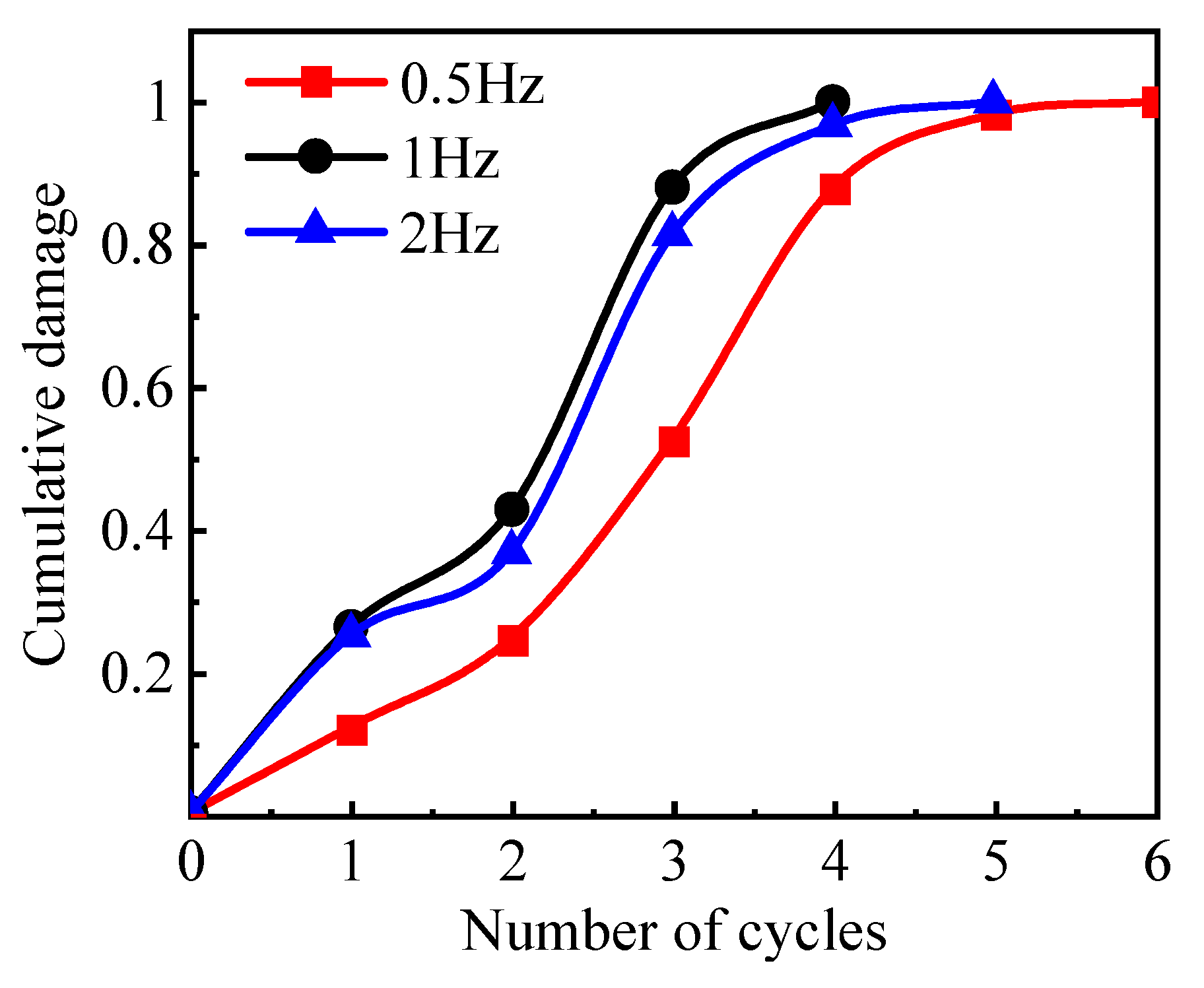
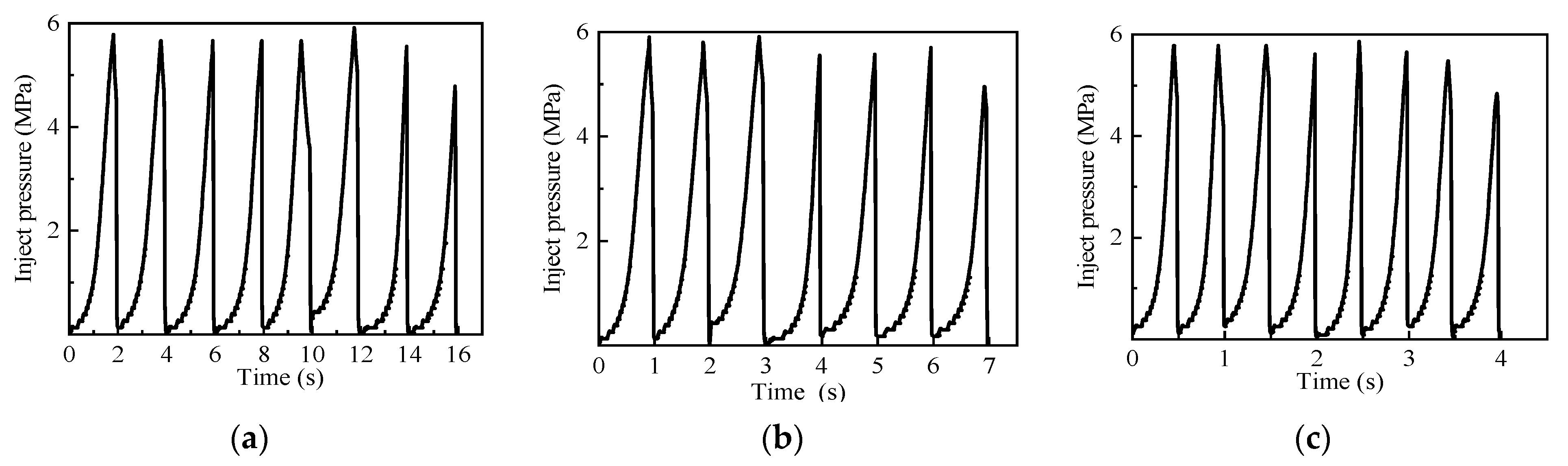
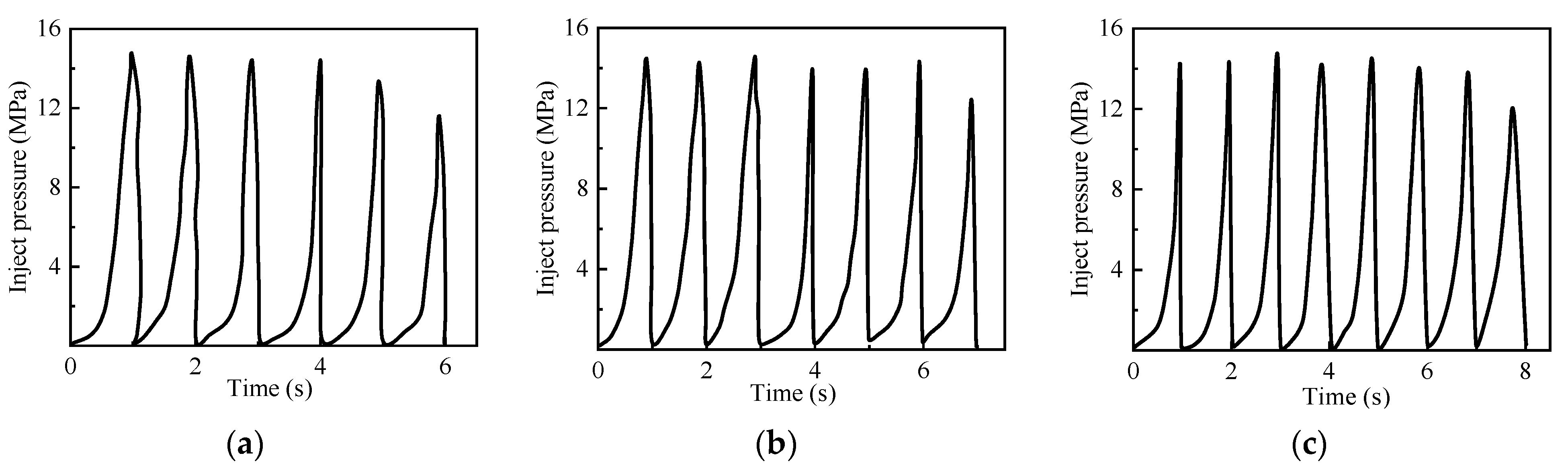
4.3.1. The Effect of the Pulse Frequency on Damage Evolution

Figure 18 displays the relationship between cumulative damage and the number of cycles at different frequencies. The cumulative damage increased gradually as the cycles increased, while the single damage decreased. This is because rock destruction is more challenging in the beginning stage. As the destruction increased, the strength of the modeled material weakened. During the intermediate stage, the destruction accumulated faster and slowed due to the previous cycles. As the number of cycles increased, destroying the model became more difficult. The damage accumulation during the middle stage increased as the number of cycles increased, slowing the damage. Although a higher frequency increased the impact, it reduced the dynamic pore pressure stability. The optimal frequency was 1 Hz, while four cycles were required for the damage to reach 1.

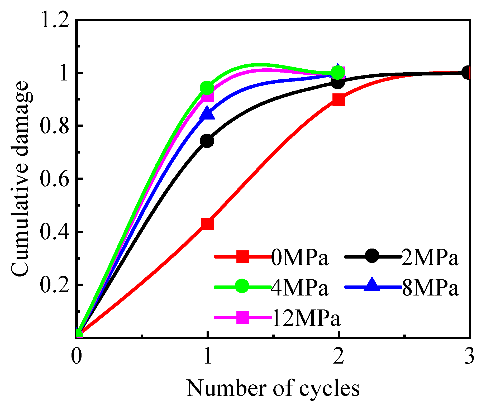
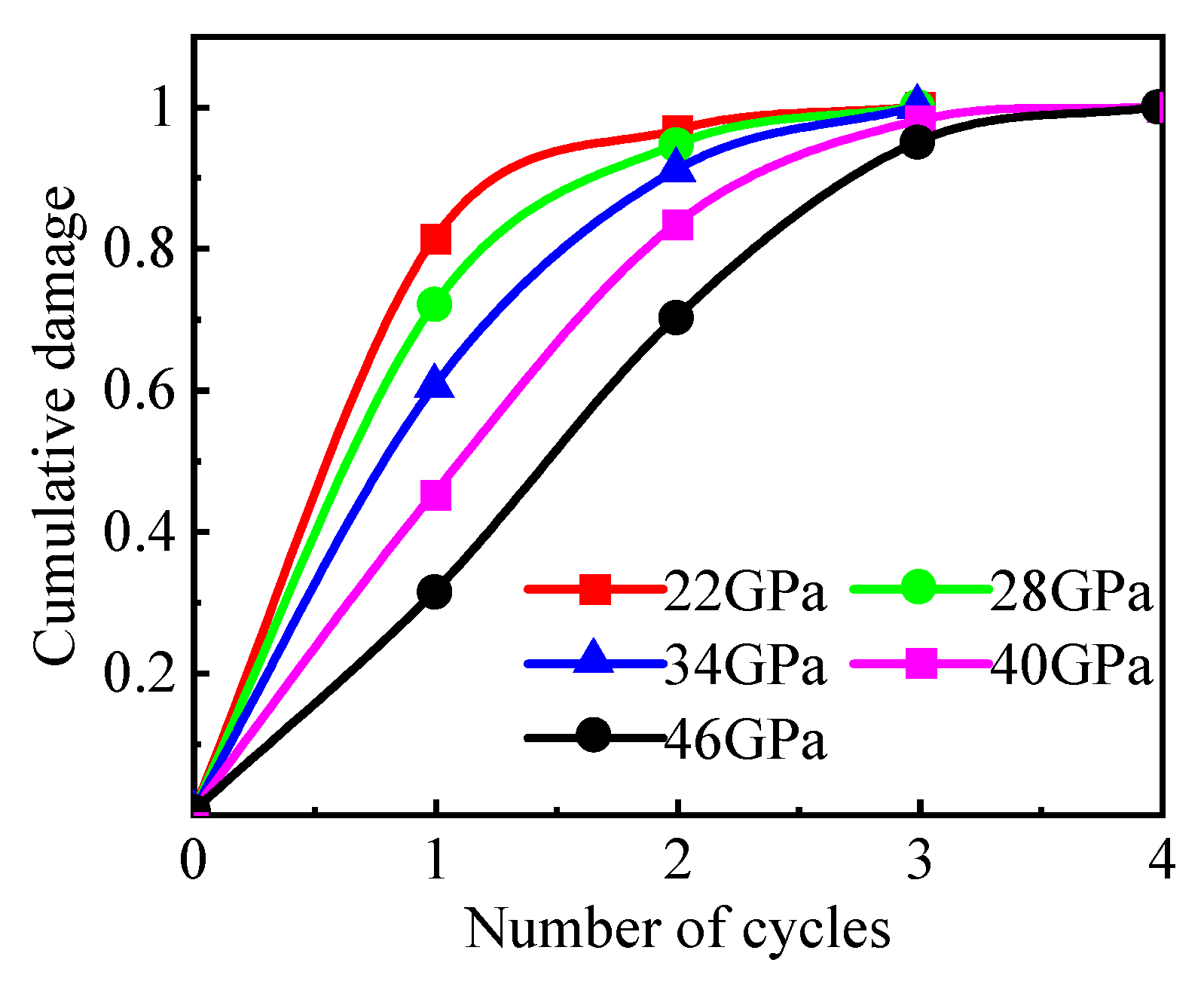
4.3.2. The Influence of Ground Stress on Damage Evolution

Figure 19 shows the relationship between the cycle number and cumulative damage at different ground stresses. At the same level, the cumulative damage increased with the number of cycles, but the increase rate slowed. The cumulative damage increased faster for larger ground stress differences, while fewer cycles were required for the damage to reach 1.

4.3.3. The Influence of Elastic Modulus Formation on Damage Evolution

Figure 20 shows the relationship between the cycle number and cumulative damage for strata with different elasticity moduli. The cumulative damage increased with the number of cycles, while single damage decreased at different elastic moduli. A smaller modulus of elasticity reduced the damage faster after each cycle, while fewer cycles were required for the cumulative damage to reach 1. This was because a smaller modulus of elasticity reduces the model strength, promoting damage occurrence.

4.3.4. The Effect of the Maximum Stress on Damage Evolution

Figure 21 shows the relationship between the number of cycles and cumulative damage at different maximum stresses. The cumulative damage increased with the number of cycles, while the single-damage variable decreased. Lower maximum stress resulted in a small starting single-damage variable, while higher stress increased the cumulative damage variable faster. Fewer cycles were required for the cumulative damage to reach 1 due to the higher principal stress and pore pressure at the same impulse load and stratigraphic conditions.

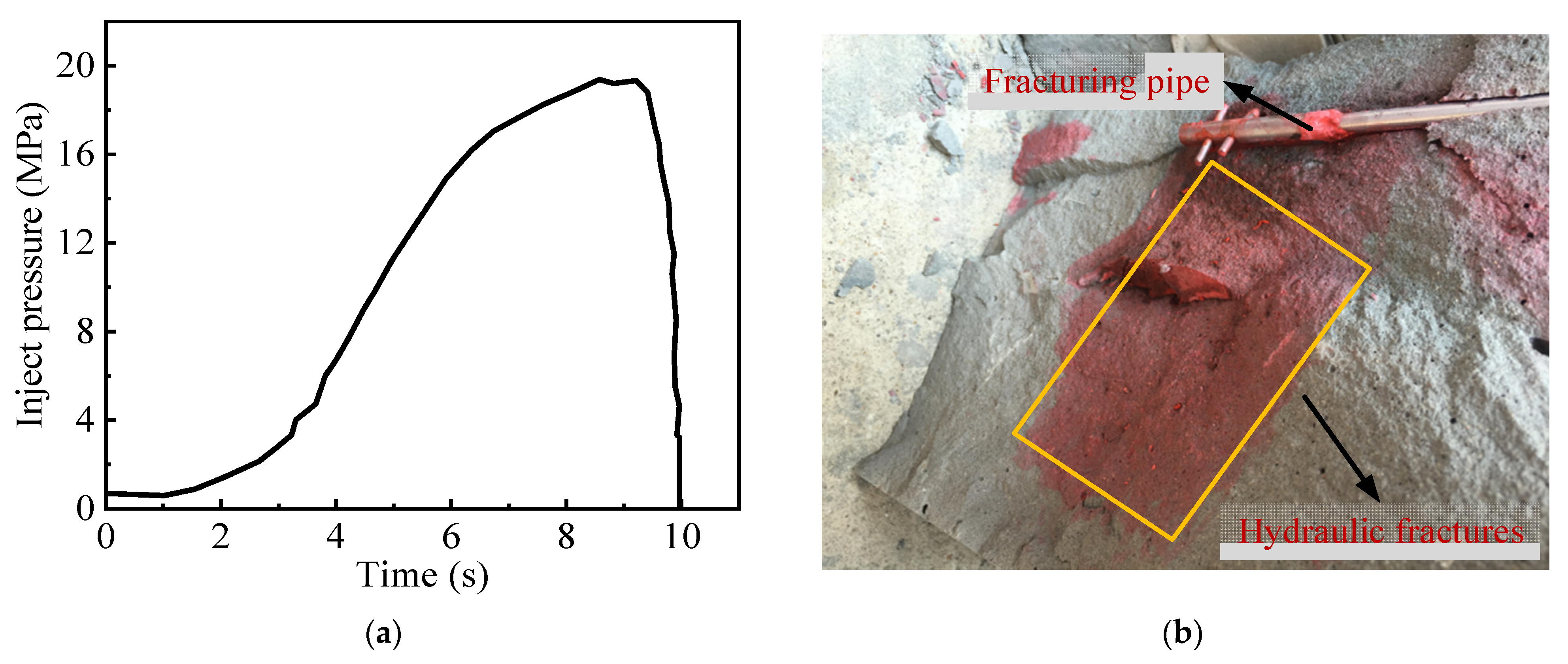
5. Experimental Research and Field Optimization

The key factors affecting initiation pressure are pulse frequency, stress amplitude, and elastic modulus. Three groups of comparative experiments were conducted to study the effect of different pulse parameters, applying 18 MPa, 15 MPa, and 25 MPa of three-directional geopathic stress.

The experiment used 300 cubic mm cement blocks as fracturing specimens, cured at room temperature for 15 d. The ratios for preparing the dense rock specimens were silicate cement:quartz sand:water (3:3:2), silicate cement:quartz sand:water (1:3:1), and silicate cement:quartz sand:water (1:3:2).

The experimental loading system (Figure 22) consisted of a triaxial servo loading system, a servo pump pressure control system, an acoustic emission spatial positioning monitoring system, and a control and monitoring system. The specimen was placed in the loading cavity, and three-way pressure was applied to simulate stratum stress. The loading process used variable frequency loading technology, starting pressure quickly via a hydraulic station and accurately pressuring the specimen via a control panel. A pulse signal generator was connected to the power control system, allowing the pump to be injected with different waveforms and frequencies to simulate water injection into the formation.

The experiment was conducted using conventional hydraulic fracturing technology. The injection pressure curves and fracture morphology are shown in Figure 23. The specimen was fractured at a starting pressure of 20 MPa, which eventually produced only one horizontal fracture. The specimen was dissected, presenting a crack in the horizontal direction.

The experiment tested the influence law of pulse frequencies on three specimens at 15 MPa amplitudes. Figure 24 shows the injection pressure curves, and Figure 25 presents the experimental results.

As shown in Figure 24, at a 1 Hz pulse frequency, the specimen fractured after seven cycles while requiring eight cycles at 0.5 Hz and 2 Hz. Pulse cycling reduced the fracture initiation pressure and complex fractures compared to conventional hydraulic fracturing.

The influence law on three specimens was verified using a 1 Hz pulse frequency at 15 MPa, 16 MPa, and 17 MPa pulse amplitudes. Figure 26 shows the injection pressure curves.

As shown in Figure 26, seven, six, and five cycles were required for specimen rupture at pulse amplitudes of 15 MPa, 16 MPa, and 17 MPa, respectively. Therefore, larger pulse amplitudes required fewer cycles.

Three specimens were examined at the same pulse frequency and amplitude to verify the influence law of varying elasticity moduli. The injection pressure curves are shown in Figure 27.

Figure 27 shows that larger specimens with higher elasticity moduli required more cycles for rupture. Numerical simulations were conducted using a model similar to the experimental specimen and dynamic material parameters, producing a 21 MPa rupture pressure during conventional hydraulic fracturing and a 15.8 MPa minimum rupture value during pulse cycling. The simulation results showed a 5% error between the simulation and experimental results, confirming the accuracy of the simulation.

Table 3. The parameters of dense reservoirs in the long seven.

Parameters	Value
Maximum horizontal principal stress	43.29 MPa
Minimum horizontal principal stress	33.62 MPa
Pore pressure	21.81 MPa
Modulus of elasticity	30 GPa
Poisson’s ratio	0.24
Permeability	$0.066\times {10}^{-3} {\mathsf{\mu }\mathrm{m}}^2$
Porosity	8.09%
Rupture pressure	45.6 MPa

lists the references for long seven-dense reservoirs in the Changqing Longdong area [37], showing characteristic parameters in each section.

Pulse-cycle hydraulic fracturing reduced the fracture pressure compared to conventional hydraulic fracturing. It required the least number of cycles at 1 Hz and was more efficient at higher pulse amplitudes. The fracture initiation pressures were calculated at different pulse frequencies and amplitudes, and relationship curves between the damage and cycle number were determined. Comparisons and analyses were conducted in static conditions, while the well parameters were optimized and designed for field use.

Figure 28a displays the damage curves versus the cycle number at different frequencies, with the number of cycles required for the damage to reach 1 varying depending on the pulse frequency. At 1 Hz, the model showed the least cycles required, at 4, compared to other frequencies. As shown in Figure 28b, the minimum damage amplitude of the model under impulse cycling was 34 MPa. The number of cycles required for the damage to reach 1 varied with the impulse amplitude, which decreased as the pulse amplitude increased. The amplitude was reduced by 24.4% compared to the static 45 MPa.

Pulse cycle hydraulic fracturing effectively reduced the fracturing pressure in practical situations. The least number of cycles required for fracturing in tight reservoirs occurred at a 1 Hz pulse frequency. The mining efficiency increased with the pulse amplitude. Therefore, pulse fracturing at a 1 Hz frequency and higher pulse amplitude was recommended to improve the efficiency.

6. Conclusions

(1) This study combines the statistical damage model and viscoelastic model, establishes the dynamic damage ontology model of dense rock according to the D-P criterion, considers the hydrodynamic continuity equation, establishes the mathematical model of pulsed hydraulic fracturing fluid–solid coupling, adopts the secondary development function of the subroutine, establishes a numerical simulation of cumulative pulsed hydraulic fracturing, and analyzes the fatigue damage mechanism under pulsed cyclic hydraulic pressure.

(2) The impact of different pulse parameters on the damage is analyzed, showing that the effect of the sinusoidal wave is 4–20% better than the triangular wave. Pulsed fluid pressure causes dynamic damage in the rock body around the borehole. The influence of frequency on rock damage increases with frequency; however, excessive frequency can cause instability in the dynamic pore pressure and limit the amount of damage that can be done. Therefore, more severe rock body damage is initially evident at a higher pulse frequency, followed by a decline. The optimal frequency is determined as 1 Hz. The rock body is gradually damaged as the number of pulse cycles increases. Compared with static hydraulic fracturing at the optimal frequency, the fracture pressure can be reduced by 26% at most.

(3) Similarity theory and the mechanical characteristics of the rock in tight reservoirs are used to create material specimens. The true triaxial hydraulic fracturing experimental system is used to perform the pulse cycle hydraulic fracturing experiments. The pulse cycle’s fracture initiation pressure is lower than that of traditional hydraulic fracturing under the same circumstances. A reduced elastic modulus and a larger pulse amplitude mean that fewer cycles are needed to fracture. Furthermore, the pulse hydraulic fracturing parameters of the on-site wells are optimized. The fracture pressure is reduced by 24% compared with that of the on-site wells, which is 45 MPa, after three cycles at a 1 Hz frequency and a 34 MPa pulse amplitude. The rupture pressure is reduced by 24%, verifying the accuracy of the numerical simulation method.

References

1. Sun, L.; Zou, C.; Jia, A.; Wei, Y.; Zhu, R.; Wu, S.; Guo, Z. Development characteristics and orientation of tight oil and gas in China. Pet. Explor. Dev. 2019, 46, 1073–1087. [Google Scholar] [CrossRef]
2. Li, B.T.; Fan, L.Y. Development of production technology in tight reservoir. Petrochem. Ind. Appl. 2021, 40, 1–6. [Google Scholar]
3. Wu, Z.Y.; Huang, Q.; Han, R.; Du, T.J. Bottleneck and Development Strategy of EOR Technology in Tight Reservoir. Chem. Eng. Des. Commun. 2020, 46, 26+41. [Google Scholar]
4. Wu, L.H.; Guo, X.Z.; Lu, W.; Zhang, Z.M.; Zhang, W.C. Influence Factors Controlling the Productivity of Horizontal Well by Volume Fracturing in Tight Oil Reservoirs—A Case Study of Dense Oil Horizontal Well in Damintun, Liaohe Oilfield. Unconv. Oil Gas 2018, 5, 56–62. [Google Scholar]
5. Miao, Z.P.; Wu, T.; Zhang, R.J.; Qu, L. Numerical Simulation on Formation Law of Complex Fracture Network by Volume Fracturing in Tight Oil Reservoir. China Pet. Mach. 2022, 50, 96–102. [Google Scholar]
6. Wang, S.; Xia, Q.; Xu, F. Investigation of collector mixtures on the flotation dynamics of low-rank coal. Fuel 2022, 327, 125171. [Google Scholar] [CrossRef]
7. Xu, F.; Wang, S.W.; Kong, R.J.; Wang, C.Y. Synergistic effects of dodecane-castor oil acid mixture on the flotation responses of low-rank coal: A combined simulation and experimental study. Int. J. Min. Sci. Technol. 2023, 33, 649–658. [Google Scholar] [CrossRef]
8. Wei, C.; Zhang, B.; Li, S.; Fan, Z.; Li, C. Interaction between Hydraulic Fracture and Pre-Existing Fracture under Pulse Hydraulic Fracturing. SPE Prod. Oper. 2021, 36, 553–571. [Google Scholar] [CrossRef]
9. Hou, M.R.; Liang, B.; Sun, W.J.; Liu, Q.; Zhao, H. Influence of mineral interface stiffness on fracture propagation law of shale hydraulic fracturing. Pet. Reser. Evaluat. Dev. 2023, 13, 100–107. [Google Scholar]
10. Matin, P.E.; Bruce, G.; Robert, G. Dynamic hydraulic stimulation and fracturing from a wellbore using pressure pulsing. Eng. Fract. Mech. 2020, 235, 107152. [Google Scholar]
11. Xi, X.; Yang, S.; McDermott, C.I.; Shipton, Z.K.; Fraser-Harris, A.; Edlmann, K. Modelling Rock Fracture Induced by Hydraulic Pulses. Rock Mech. Rock Eng. 2021, 54, 3977–3994. [Google Scholar] [CrossRef]
12. Xia, Y.; Zhang, C.; Zhou, H.; Hou, J.; Su, G.; Gao, Y.; Liu, N.; Singh, H.K. Mechanical behavior of structurally reconstructed irregular columnar jointed rock mass using 3D printing. Eng. Geol. 2020, 268, 105509. [Google Scholar] [CrossRef]
13. Xia, Y.; Zhang, C.; Zhou, H.; Chen, J.; Gao, Y.; Liu, N.; Chen, P. Structural characteristics of columnar jointed basalt in drainage tunnel of Baihetan hydropower station and its influence on the behavior of P-wave anisotropy. Eng. Geol. 2019, 264, 105304. [Google Scholar] [CrossRef]
14. Xia, Y.; Liu, B.; Zhang, C.; Liu, N.; Zhou, H.; Chen, J.; Tang, C.; Gao, Y.; Zhao, D.; Meng, Q. Investigations of mechanical and failure properties of 3D printed columnar jointed rock mass under true triaxial compression with one free face. Geomech. Geophys. Geo-Energy Geo-Resour. 2022, 8, 26. [Google Scholar] [CrossRef]
15. Zhao, D.; Xia, Y.; Zhang, C.; Liu, N.; Tang, C.; Singh, H.K.; Chen, J.; Wang, P. A New Method to Investigate the Size Effect and Anisotropy of Mechanical Properties of Columnar Jointed Rock Mass. Rock Mech. Rock Eng. 2023, 56, 2829–2859. [Google Scholar] [CrossRef]
16. Zhao, D.; Xia, Y.; Zhang, C.; Tang, C.; Zhou, H.; Liu, N.; Singh, H.K.; Zhao, Z.; Chen, J.; Mu, C. Failure modes and excavation stability of large-scale columnar jointed rock masses containing interlayer shear weakness zones. Int. J. Rock Mech. Min. Sci. 2022, 159, 105222. [Google Scholar] [CrossRef]
17. Frash, L.P.; Gutierrez, M.; Hampton, J. Laboratory-Scale-Model Testing of Well Stimulation by Use of Mechanical-Impulse Hydraulic Fracturing. SPE J. 2015, 20, 536–549. [Google Scholar] [CrossRef]
18. Wu, J.; Zhang, S.; Cao, H.; Zheng, M.; Qu, F.; Peng, C. Experimental investigation of crack dynamic evolution induced by pulsating hydraulic fracturing in coalbed methane reservoir. J. Nat. Gas Sci. Eng. 2020, 75, 103159. [Google Scholar] [CrossRef]
19. Zhao, K.; Li, R.; Lei, H.; Gao, W.; Zhang, Z.; Wang, X.; Qu, L. Numerical Simulation of Influencing Factors of Hydraulic Fracture Network Development in Reservoirs with Pre-Existing Fractures. Processes 2022, 10, 773. [Google Scholar] [CrossRef]
20. Lu, C.; Ma, L.; Guo, J.; Zhao, L.; Xu, S.; Chen, B.; Zhou, Y.; Yuan, H.; Tang, Z. Fracture Parameters Optimization and Field Application in Low-Permeability Sandstone Reservoirs under Fracturing Flooding Conditions. Processes 2023, 11, 285. [Google Scholar] [CrossRef]
21. Cappa, F.; Guglielmi, Y.; Rutqvist, J.; Tsang, C.; Thoraval, A. Estimation of fracture flow parameters through numerical analysis of hydromechanical pressure pulses. Water Resour. Res. 2008, 44, 7015. [Google Scholar] [CrossRef]
22. Chen, J.Z.; Li, X.B.; Cao, H.; Zhu, Q.Q. Experimental study on the mechanism of coupled dynamic–static fracturing on damage evolution and crack propagation in tight shale. Energy Rep. 2022, 8, 7037–7062. [Google Scholar] [CrossRef]
23. Xie, J.N.; Xie, J.; Ni, G.H.; Rahman, S.; Sun, Q.; Wang, H. Effects of pulse wave on the variation of coal pore structure in pulsating hydraulic fracturing process of coal seam. Fuel 2020, 264, 116906. [Google Scholar]
24. Zhuang, L.; Kim, K.Y.; Jung, S.G.; Diaz, M.; Min, K.-B.; Zang, A.; Stephansson, O.; Zimmermann, G.; Yoon, J.-S.; Hofmann, H. Cyclic hydraulic fracturing of pocheon granite cores and its impact on breakdown pressure, acoustic emission amplitudes and injectivity. Int. J. Rock Mech. Min. Sci. 2019, 122, 104065. [Google Scholar] [CrossRef]
25. Stephansson, O.; Semikova, H.; Zimmermann, G.; Zang, A. Laboratory Pulse Test of Hydraulic Fracturing on Granitic Sample Cores from Aspo HRL, Sweden. Rock Mech. Rock Eng. 2018, 52, 629–633. [Google Scholar] [CrossRef]
26. Diaz, M.B.; Kim, K.Y.; Jung, S.G. Effect of frequency during cyclic hydraulic fracturing and the process of fracture development in laboratory experiments. Int. J. Rock Mech. Min. Sci. 2020, 134, 104474. [Google Scholar] [CrossRef]
27. Wu, J.J.; Wu, J.Z.; Zhou, P.Y.; Li, X.X. Analysis about Feasibility of Multiple Pulses Loading Fracturing in Low Permeability Coal Reservoir. Coal Technol. 2017, 36, 135–138. [Google Scholar]
28. Zhang, Z.H. High Pressure Pulsed Hydra-jet Fracturing in CBM. J. Chengde Pet. Coll. 2020, 22, 32–37. [Google Scholar]
29. Nie, C.P.; Lan, J.P.; Wang, Z.W.; Zhang, M.; Xu, H.X.; Yin, G.Y. Downhole Low Frequency Hydraulic Pulsing Fracturing Technology and Its Application. Drill. Prod. Technol. 2021, 44, 38–42. [Google Scholar]
30. He, P.; Lu, Z.; Deng, Z.; Huang, Y.K.; Qin, D.W.; Ouyang, L.M.; Li, M.L. An advanced hydraulic fracturing technique: Pressure propagation and attenuation mechanism of step rectangular pulse hydraulic fracturing. Energy Sci. Eng. 2023, 11, 299–316. [Google Scholar] [CrossRef]
31. Wei, C.; Li, S.; Yu, L.; Zhang, B.; Liu, R.; Pan, D.; Zhang, F. Study on Mechanism of Strength Deterioration of Rock-Like Specimen and Fracture Damage Deterioration Model Under Pulse Hydraulic Fracturing. Rock Mech. Rock Eng. 2023, 56, 4959–4973. [Google Scholar] [CrossRef]
32. Anjun, J.; Shixiang, T.; Huaying, L. Study on Crack Penetration Induced by Fatigue Damage of Low Permeability Coal Seam under Cyclic Loading. Energies 2022, 15, 13. [Google Scholar]
33. Hua, D.J.; Liu, T. Study on cyclic impact experiment for rocks under static stress state and the failure mode. Non-Ferr. Metals 2014, 66, 52–57. [Google Scholar]
34. Tang, W.; Zhao, X.B.; Lei, J.Y.; Yuan, B.; Liu, H.W. Numerical Simulation on the Size Effect of Compressive Strength and Deformation Parameters of Rock Materials Under Different Confining Pressures. Geol. J. China Univ. 2016, 22, 580–588. [Google Scholar]
35. Gao, H.; Huang, H.-Z.; Lv, Z.; Zuo, F.-J.; Wang, H.-K. An improved Corten-Dolan’s model based on damage and stress state effects. J. Mech. Sci. Technol. 2015, 29, 3215–3223. [Google Scholar] [CrossRef]
36. Xie, H.P.; Chen, Z. Exploration of continuum damage mechanics modelling of rocks. J. China Coal Soc. 1988, 1988, 33–42. [Google Scholar]
37. Wu, T.; Wang, Y.; Fu, B.; Wu, P. A new method of multi-scale fracture identification in tight gas sandstone reservoir. Geosyst. Eng. 2018, 22, 112–118. [Google Scholar] [CrossRef]
Figure 1. The time-damage model.
Processes 11 03398 g001
Figure 2. The stress displacement criterion for cohesive element softening.
Processes 11 03398 g002
Figure 3. The study area and model.
Processes 11 03398 g003
Figure 4. The cloud maps of the different pulse-loading frequencies around the borehole: (a) The maximum principal stress in the plane. (b) Pore pressure. (c) Damage.
Processes 11 03398 g004
Figure 5. Variation rule around borehole under different pulse loading frequencies: (a) The maximum principal stress in the plane. (b) Pore pressure. (c) Damage.
Processes 11 03398 g005
Figure 6. The cloud maps of the differential ground stress around the borehole: (a) The maximum principal stress in the plane. (b) Pore pressure. (c) Damage.
Processes 11 03398 g006
Figure 7. Variation rule around borehole under different ground stresses: (a) The maximum principal stress in the plane. (b) Pore pressure. (c) Damage.
Processes 11 03398 g007
Figure 8. The cloud maps of the area around the borehole at different modulus of elasticities: (a) The maximum principal stress in the plane. (b) Pore pressure. (c) Damage.
Processes 11 03398 g008
Figure 9. Variation rule around the borehole under a different modulus of elasticities: Modulus of elasticity. (a) The maximum principal stress in the plane. (b) Pore pressure. (c) Damage.
Processes 11 03398 g009
Figure 10. The cloud maps of the different maximum stresses around the borehole: (a) The maximum principal stress in the plane. (b) Pore pressure. (c) Damage.
Processes 11 03398 g010
Figure 11. Variation rule around borehole under different maximum stresses: (a) The maximum principal stress in the plane. (b) Pore pressure. (c) Damage.
Processes 11 03398 g011
Figure 12. The waveform effect at different frequencies: (a) The maximum principal stress in the plane. (b) Pore pressure. (c) Damage.
Processes 11 03398 g012
Figure 13. The waveform effect of the different ground stress differences: (a) The maximum principal stress in the plane. (b) Pore pressure. (c) Damage.
Processes 11 03398 g013
Figure 14. The waveform effect at different maximum stresses: (a) The maximum principal stress in the plane. (b) Pore pressure. (c) Damage.
Processes 11 03398 g014
Figure 15. The subroutine flowchart.
Processes 11 03398 g015
Figure 16. The damage cloud of the comparison between conventional and pulse fracturing.
Processes 11 03398 g016
Figure 17. The cumulative damage curve of pulse fracturing at 37 MPa.
Processes 11 03398 g017
Figure 18. The curve of the cumulative damage variable versus the number of cycles at different frequencies.
Processes 11 03398 g018
Figure 19. The cumulative damage variables versus the number of cycles at different ground stresses.
Processes 11 03398 g019
Figure 20. The cumulative damage variable versus the number of cycles for different elasticity moduli.
Processes 11 03398 g020
Figure 21. The cumulative damage variables versus the number of cycles at different maximum stresses.
Processes 11 03398 g021
Figure 22. A schematic diagram of the true triaxial core injection experiment system.
Processes 11 03398 g022
Figure 23. Conventional injection: (a) injection curves, (b) final crack patterns.
Processes 11 03398 g023
Figure 24. The injection pressure curves at different frequencies: (a) 0.5 Hz. (b) 1 Hz. (c) 2 Hz.
Processes 11 03398 g024
Figure 25. The experimental results of pulse cycle hydraulic fracturing.
Processes 11 03398 g025
Figure 26. The injection pressure curves for the different pulse amplitudes: (a) 15 MPa. (b) 16 MPa. (c) 17 MPa.
Processes 11 03398 g026
Figure 27. The injection pressure curves for the different stratigraphic elasticity moduli: (a) 18 GPa. (b) 20 GPa. (c) 22 GPa.
Processes 11 03398 g027
Figure 28. The damage versus the number of cycles: (a) Different frequencies. (b) Different amplitudes.
Processes 11 03398 g028