Performance Evaluation of Chiller Fault Detection and Diagnosis Using Only Field-Installed Sensors

Abstract

Owing to the rapid expansion of data science, data-driven methods have emerged as a dominant trend in chiller fault detection and diagnosis (FDD). Most of these methods prioritize feature selection to achieve optimal diagnostic performance. However, on-site research indicates a common installation of a limited number of sensors, coupled with a necessity to minimize diagnostic costs. This discrepancy between existing research’s feature selection principles and the current on-site sensor installation status presents a significant challenge. To facilitate the practical implementation of data-driven methods in real chiller units, this study addresses a critical question: under the constraint of limited on-site sensor installations, what is the optimal performance achievable by data-driven methods and their improved versions? To answer this, only features derived from commonly installed sensors on field chillers are chosen as indicators for typical chiller faults. The FDD performance of six frequently used data-driven methods, namely, back-propagation neural network, convolutional neural network, support vector machine, support vector data description, Bayesian network, and random forest, along with their improved versions, is comprehensively evaluated and validated using experimental data, considering four evaluation metrics. The conclusions drawn in this paper provide valuable insights for users/manufacturers with limited or no budget, detailing the best achievable diagnostic performance for each typical fault and offering guidance for those aiming to further enhance FDD performance.

1. Introduction

The world is currently grappling with two major challenges: energy and the environment. According to research conducted by the International Institute of Refrigeration, there are approximately 3 billion refrigeration, air conditioning, and heat pump units worldwide, collectively consuming nearly 17% of electricity [1]. Recognizing the significance of this issue, China has placed great emphasis on the need to curb carbon emissions and aims to reach the peak of emissions by 2030, followed by achieving carbon neutrality by 2060.

Within China, the heating, ventilating, and air conditioning (HVAC) sector constitutes a substantial portion of energy consumption, accounting for around 60% of total building energy usage [2]. Chillers, specifically, contribute to 40% of the energy consumed by buildings [3]. However, chiller failures can result in additional energy wastage, reduced equipment lifespan, compromised indoor comfort, and evenenviron mental pollution through refrigerant leakage [4]. These consequences underscore the importance of addressing fault detection and diagnosis (FDD) in chiller systems.

Over the past few decades, extensive research has been carried out in the field of chiller FDD, as comprehensively summarized and reviewed by Zhao et al. [5] and Mirnaghi et al. [6]. Many scholars have introduced numerous methods and validated them using experimental data, demonstrating their excellent performance. These methods have been categorized into different types from varying perspectives. For example, Wei et al. [7] classified FDD methods as white-box-based, grey-box-based, and black-box-based, while Katipamula and Brambley [4], and later in their subsequent work [8], categorized them as quantitative model-based, qualitative model-based, or process history (data-driven). Indeed, these classifications do not have significant differences in essence.

Currently, there is a prevailing trend in the development of FDD methods applied to chillers: an increasing number of methods are leveraging data-driven algorithms. This shift is attributed to the rapid expansion of data science in recent years. Notably, recent review articles by Mirnaghi et al. [6], Wei et al. [7], Shi et al. [9], Chen et al. [10], and Chen et al. [11] have concentrated on data-driven FDD. Summarizing insights from these reviews reveals that almost 80% of the recently proposed methods fall under the category of data-driven approaches. For FDD within the HVAC domain, the following six methods are some of the most frequently employed data-driven approaches. The first typical approach is neural networks, with back-propagation neural network (BPNN) and convolutional neural network (CNN) being widely used training algorithms. They have been applied to anomaly detection for HVAC systems in the work of Borda et al. [12], and to FDD of chillers in the works of Gao et al. [13] and Gao et al. [14]. The second typical data-driven approach is support vector machine (SVM), which has been employed for FDD of HVAC systems in works by Han et al. [15], Fan et al. [16], Amir et al. [17], and Van et al. [18]. Support vector data description (SVDD) is the third typical data-driven approach, and its application to FDD in the HVAC field can be found in works by Zhao et al. [19], Chen et al. [20], and Zhang et al. [21]. Bayesian network (BN) is the fourth typical data-driven approach, and its application to FDD of HVAC systems is demonstrated in works by Wang et al. [22,23], Ng et al. [24], Li et al. [25], and Liu et al. [26]. Lastly, random forest (RF) represents the fifth typical data-driven approach, and its application to FDD of HVAC systems can be observed in works by Han et al. [15] and Li et al. [27]. When applying these approaches to the FDD of chillers, their performance has been extensively validated in the existing literature. Published studies report diagnostic accuracies exceeding 90% for nearly all typical chiller faults, with some reaching as high as 99%. However, such exceptional diagnostic performance is contingent upon having an ample set of features. The question of whether such excellent diagnostic performance can still be achieved when the available features are extremely limited warrants in-depth investigation.

In addition to the previously mentioned widely employed methods, there are several other approaches in use, including autoencoder [28], semi-supervised learning [29], as well as unsupervised learning methods such as principal component analysis [30], association rules mining [31], and cluster analysis [32], and other novel methods, e.g., domain adaptation networks with parameter-free adaptively rectified linear units [33], dual-path mixed-domain residual threshold networks [34], and wavelet neural network [35].

Data-driven FDD methods, in general, rely on identifying patterns in the measures of selected features to detect and diagnose faults [5]. Therefore, the specific quantity and types of features used in the training process significantly affect the accuracy of these models. In the context of chiller FDD, numerous efforts have been made to identify suitable features. Comstock et al. [36], Zhou et al. [37], and Zhao et al. [19] selected 14, 8, and 16 features, respectively, from the original features using experimental analysis, sensitivity analysis, and expert knowledge. Bai et al. [38] employed a feature recognition model and kernel discriminant analysis to select 12 features indicative of the chiller’s healthy conditions. Zhang et al. [39] developed a hybrid algorithm that combines filter and wrapper methods to generate an optimal feature set with the ideal number of features. Han et al. [40] and Gao et al. [41], based on optimal algorithms and global sensitivity analysis, selected 8 and 14 of the most effective features from an initial set of 64 features, respectively. Yan et al. [42], using cost-sensitive classification accuracy, identified an optimal subset of 16 features for chiller FDD. Nevertheless, the majority of data-driven methods focus on selecting features to achieve optimal diagnostic performance, often overlooking the practical constraints imposed by on-site sensor installations.

Analysis based on on-site research reveals a dual scenario: not only are a limited number of sensors typically installed on-site, but there is also a demand for minimizing diagnostic costs. Two comprehensive studies by Wang et al. [43] and Zhao et al. [44] investigated field chillers, encompassing 22 chillers and 14 chillers located in China, America, and Italy, respectively. The findings from these field investigations confirm that only a few sensors are generally installed in chillers, primarily for operational regulation and control. The reluctance of users and manufacturers to install an extensive array of sensors in chillers stems from cost considerations. Furthermore, for FDD to achieve a cost-to-benefit ratio comparable to critical applications such as nuclear power plants, aircraft, and chemical process plants, it is imperative to minimize the cost of FDD. This necessitates reducing the installation cost of sensors to maximize economic benefits.

The disparity between the existing research’s feature selection principles and the current on-site sensor installation status has given rise to a significant paradox. The practical reality of having a limited number of on-site sensors and the imperative for cost-effective applications strongly constrains the types and quantity of features that FDD methods can utilize. This disconnection results in the features chosen by the majority of methods outlined in the literature not aligning with the actual sensor installations on chillers in the field. Such incongruence stands as a fundamental impediment to the widespread application of proposed FDD methods in practical scenarios. For instance, to attain optimal diagnostic performance, a considerable number of data-driven methods incorporate features measured by sensors that are not typically found in field chillers. Some even resort to using virtual features solely obtained in controlled laboratory environments. For instance, water flow is a key sensitive feature as it directly indicates abnormal water flow and has been used in many works [40,41,42]. Still, it is not commonly installed due to high installation and maintenance costs. Even relatively inexpensive sub-cooling sensors, used in other works [19,36,43], are not typically found in the field, emphasizing the cost considerations of users and manufacturers. In laboratory settings, auxiliary loops may be designed to provide precise control for simulating faults, but the features from these auxiliary loops are not present in an actual chiller. These features are referred to as virtual features and are utilized in some works [40,41,42].

Through the aforementioned analysis, it is clear that data-driven methods are a prevailing trend, and the restricted installation of on-site sensors is a practical reality. To facilitate the practical implementation of data-driven methods in actual chiller units, several questions need to be addressed: under the constraint of limited on-site sensor installations, what is the optimal performance achievable by data-driven methods and their improved versions? This question takes into consideration both economic constraints and the cost-to-benefit ratio of FDD. Addressing this question serves two valuable purposes: (1) informing users/manufacturers with limited or no budget about the best achievable diagnostic performance for each typical fault, and (2) offering guidance for users/manufacturers aiming to further improve FDD performance. To tackle this question and attain the corresponding beneficial outcomes, only features derived from commonly installed sensors on field chillers are chosen as indicators for typical chiller faults. These selected features encompass 8 directly measured features and an additional 10 calculated features. Seven typical chiller faults are considered, and a comprehensive evaluation across six frequently used data-driven methods (BPNN, CNN, SVM, SVDD, BN, and RF) is conducted using these selected features, taking into account four evaluation metrics.

The major contributions of this work are as follows:

(1)

Whether mainstream data-driven FDD methods can still achieve the expected performance when relying solely on features obtained from sensors universally installed on-site is investigated;

(2)

For each fault, insights into the optimal FDD performance achievable by data-driven models using solely field-installed sensors are provided;

(3)

The conclusions drawn provide guidance on whether additional sensor installations are necessary, serving as a reference for optimizing the cost–benefit ratio in chiller FDD.

2. Methods and Materials

2.1. Frameworks of Data-Driven FDD Methods

According to classification mechanisms, FDD approaches can be classified into one-class classification-based and multi-class classification-based ones. Figure 1 and Figure 2 illus trate the FDD frameworks for one-class classification and multi-class classification, respectively. Among the six data-driven methods considered in this study, SVDD and BN are used as one-class classification methods, while BPNN, CNN, SVM, and RF are employed as multi-class classification methods.

For the one-class classification-based methods, the FDD problem is transformed into a single-class classification problem. Faults are detected and diagnosed step by step. The process involves sequentially identifying the presence or absence of individual fault conditions. Once a fault is detected, the subsequent step focuses on diagnosing the specific fault.

On the contrary, the multi-class classification-based methods transform the FDD problem into a multi-class classification problem. They simultaneously detect and diagnose faults using a single-step completion strategy. This involves directly classifying the system into fault classes or determining the presence of specific fault conditions in a single classification step. These approaches provide a more immediate detection and diagnosis of faults, without the need for sequential steps.

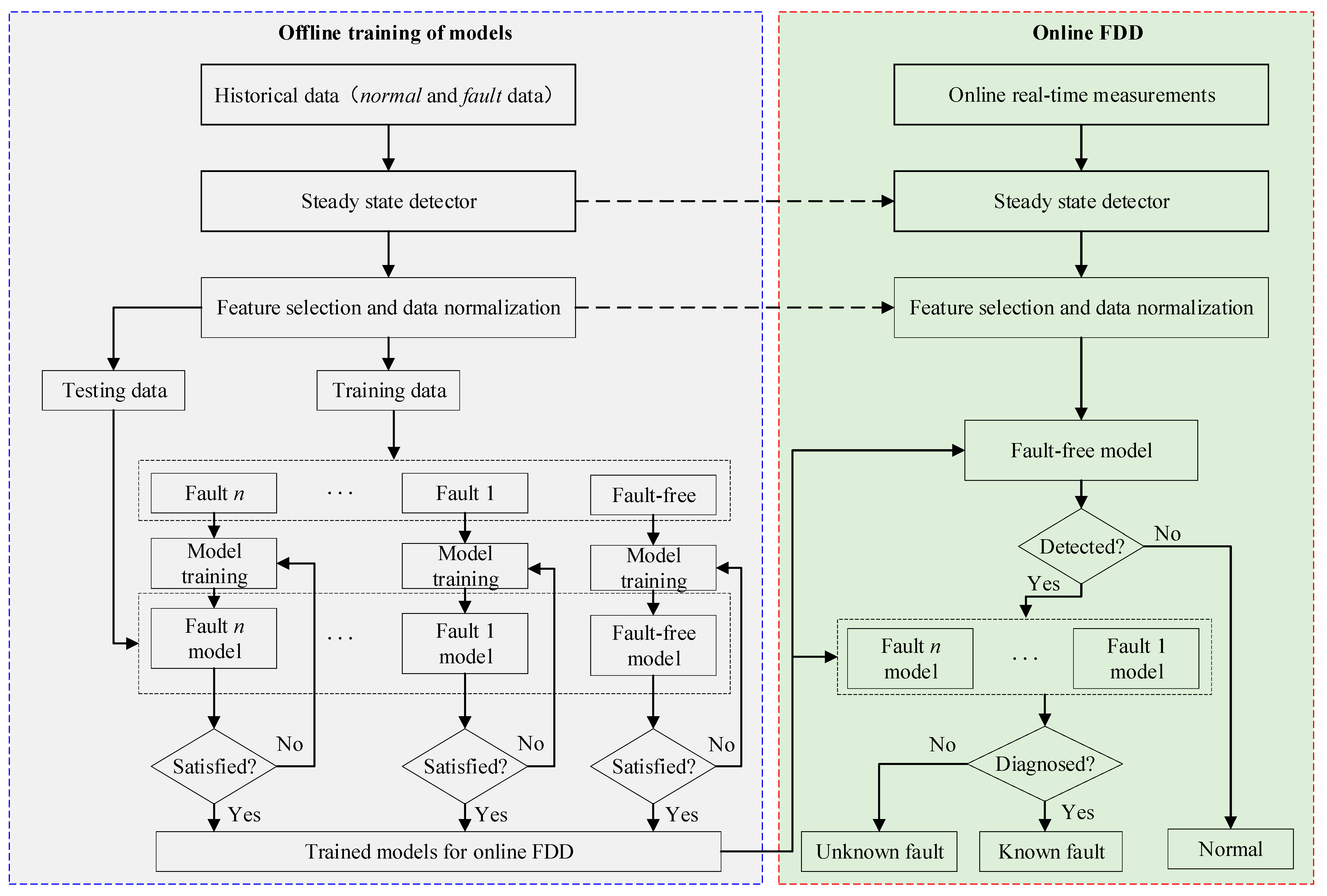
2.1.1. One-Class Classification

As depicted in Figure 1, the FDD method employing a one-class classification mechanism consists of two main parts: offline model training and online FDD.

During the offline model training process, historical data containing fault-free and faulty instances are collected from the database. These data undergo pre-processing steps. Firstly, a steady-state filter is applied to remove obvious outliers and dynamic data. Secondly, appropriate features are selected to effectively represent the health states of the system. Thirdly, the steady-state data are normalized to eliminate any discrepancies in magnitude among them. Subsequently, the pre-processed data are divided into training and testing sets. The training set is used to train the models, while the testing set evaluates the performance of the trained models. Finally, the models are trained according to predetermined principles and criteria.

In the online FDD process, the trained models are utilized for FDD in real time. Firstly, the online real-time data undergo the same pre-processing steps as those during the offline training process. Then, the fault-free model is applied to detect faults. If a fault is detected, the real-time data are input into the trained models corresponding to each known fault, one by one. This allows for the specific fault to be determined based on the outputs of the trained models.

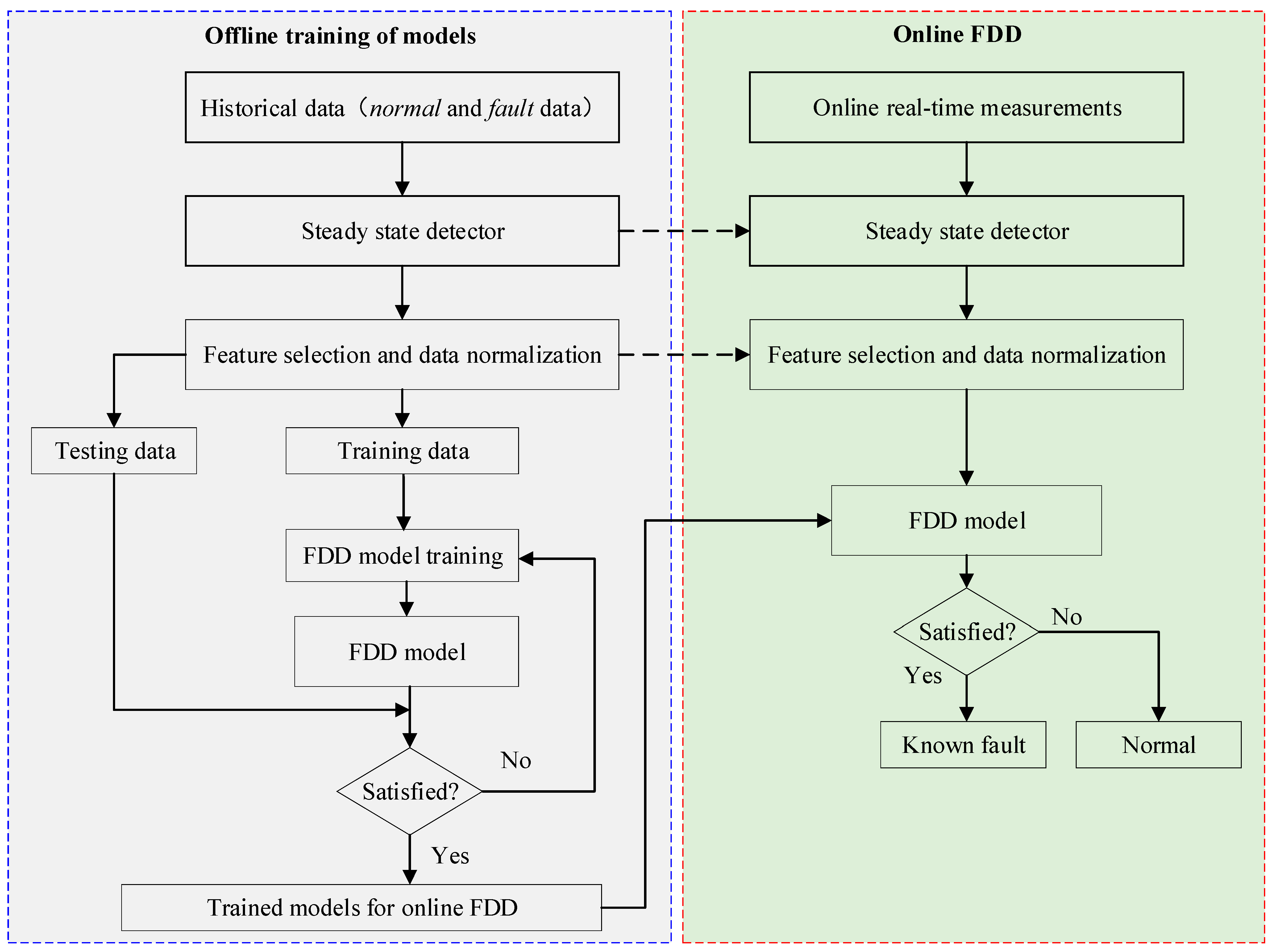
2.1.2. Multi-Class Classification

As illustrated in Figure 2, the FDD method utilizing a multi-class classification mechanism also comprises two main components: offline model training and online FDD.

The data pre-processing, feature selection, and data normalization steps remain the same for both the one-class classification and multi-class classification methods. The differences between them can be summarized as follows:

Offline model training: for the multi-class classification methods, a single (or integrated) FDD model is trained to handle both fault detection and diagnosis. The training process focuses on optimizing this specific model to accurately classify the system’s states. In contrast, the one-class classification methods involve training multiple models, each dedicated to detecting and diagnosing a specific fault condition;

Online FDD process: during the online FDD phase, the trained models for the multi-class classification methods are applied to real-time data for both fault detection and diagnosis. The significant distinction is that the FDD results are generated simultaneously. In other words, the models provide immediate assessment on the system’s status, indicating whether it is operating normally or experiencing a specific fault.

2.2. Investigation of Field Chiller Onboard Sensors

The knowledge regarding the sensors commonly installed on field chillers has been extensively investigated in previous studies. Wang et al. [43] conducted a survey in which they randomly selected and investigated 22 machine rooms with chillers in Shaanxi province, China. Similarly, Zhao et al. [44] conducted a survey in which they randomly selected and investigated 14 field chillers from three different manufacturers. The 14 field chillers were located in four cities of America and Italy. Interestingly, both studies reported consistent results.

After conducting the investigations, it was revealed that field chillers commonly have eight sensors installed. These sensors and their respective features are listed in

Table 1. The respective features measured by the commonly installed sensors.

No.	Designation	Description	Formulation
1	$TEI$	Entering evaporator water temperature	Direct measurement
2	$TEO$	Leaving evaporator water temperature	Direct measurement
3	$TCI$	Entering condenser water temperature	Direct measurement
4	$TCO$	Leaving condenser water temperature	Direct measurement
5	$P_{in}$	Compressor input power	Direct measurement
6	$TRE/PRE$	Evaporating temperature/pressure	Direct measurement
7	$TRC/PRC$	Condensing temperature/pressure	Direct measurement
8	$T{R}_{dis}$	Refrigerant discharge temperature	Direct measurement

. Furthermore, additional features can be derived by calculating specific parameters based on the measurements obtained from the sensors in Table 1. In theory, an extensive array of features can be derived from the features presented in Table 1. However, from a statistical standpoint, attempting to list all these features is both impractical and unnecessary. In this paper, additional features are generated following a set of key principles: (1) These features can be acquired through straightforward calculations. Given the demands of real-world on-site applications, elaborate computations necessitate extra computing and storage resources, which inevitably drive up the cost of FDD implementations; (2) These features hold significant thermodynamic significance and can effectively characterize the thermodynamic performance of chillers; 3) These features are frequently employed by other researchers, and their efficacy has been validated in prior studies. Adhering to these three guiding principles, the additional features are identified and outlined in

Table 2. The features derived from these parameters in Table 1.

No.	Designation	Description	Formulation
1	$\mathrm{\Delta }{T}_e$	Evaporator water temperature difference	$\mathrm{\Delta }{T}_e=TEI-TEO$
2	$\mathrm{\Delta }{T}_c$	Condenser water temperature difference	$\mathrm{\Delta }{T}_c=TCO-TCI$
3	$LMT{D}_e$	Logarithmic mean temperature difference of evaporator	$LMT{D}_e=\frac{TEI-TEO}{\ln \left(\frac{TEI-TRE}{TEO-TRE}\right)}$
4	$LMT{D}_e$	Logarithmic mean temperature difference of condenser	$LMT{D}_c=\frac{TCO-TCI}{\ln \left(\frac{TRC-TCI}{TRC-TCO}\right)}$
5	$TEA$	Evaporator approach temperature	$TEA=TEO-TRE$
6	$TCA$	Condenser approach temperature	$TCA=TRC-TCO$
7	$Ts{h}_{dis}$	Refrigerant discharge superheat temperature	$Ts{h}_{dis}=T{R}_{dis}-TRC$
8	${\xi }_{sat,c}$	Heat transfer efficiency in saturation section of condenser	${\xi }_{sat,c}=\frac{TCO-TCI}{TRC-TCI}$
9	${\xi }_{sh,c}$	Heat transfer efficiency in superheat section of condenser	${\xi }_{sh,c}=\frac{Ts{h}_{dis}}{T{R}_{dis}-TCO}$
10	${\xi }_{sat,e}$	Heat transfer efficiency in saturation section of evaporator	${\xi }_{sat,e}=\frac{Ts{h}_{dis}}{T{R}_{dis}-TCO}$

.

Based on the investigation results, the features shown in Table 1 and Table 2, obtained from the commonly installed sensors, are selected to indicate the typical faults of a chiller. Considering these field constraints, the question whether the mainstream data-driven FDD methods can still be effective to obtain an expected performance is addressed.

2.3. Experimental Data and Model Evaluation

In this section, the performance of current mainstream data-driven methods is assessed by applying them to an experimental chiller. The chiller is a centrifugal water-cooled chiller, as reported in ASHRAE RP-1043 [45]. The FDD performance is evaluated comprehensively by using four evaluation indexes.

2.3.1. Experimental Data

The experimental data from ASHRAE RP-1043 [45] are utilized to evaluate the FDD performance of the data-driven methods. ASHRAE RP-1043 represents the first phase research project initiated by ASHRAE in the late 1990s, with the aim of providing a standardized evaluation tool for chiller FDD methods. This experiment was conducted on a centrifugal water-cooled chiller to collect a substantial amount of data encompassing both normal operating conditions and various fault scenarios. These data have become a widely adopted benchmark dataset and have been utilized by numerous researchers to assess and validate their proposed FDD methods.

The chiller is a centrifugal water-cooled chiller with a cooling capacity of 316 kW, utilizing R134a as the refrigerant. The condenser and evaporator are both shell and tube heat exchangers. Seven typical chiller faults were deliberately induced during the experiment, including reduced condenser water flow (RedCdW), reduced evaporator water flow (RedEvW), refrigerant leakage (RefLeak), refrigerant overcharge (RefOver), condenser fouling (CdFoul), non-condensable gas in refrigerant (NcG), and excess oil (ExOil). Each fault condition was evaluated at four severity levels (SL-1, SL-2, SL-3, and SL-4), representing increasing severity from 10% to 40%.

The experimental measurements were collected under 27 distinct operating conditions, achieved by varying the evaporator water leaving temperature, condenser water entering temperature, and the cooling load. A total of 64 measurements were recorded at 10-second intervals during each operating condition. For more detailed information regarding the experimental setup and data collection process, refer to Ref. [45].

2.3.2. Feature Selection and Data Pre-Processing

Based on the investigation results presented in Section 2.2, the features listed in Table 1 and Table 2 are derived from common field-installed sensors. To address the question of whether mainstream data-driven FDD methods can still effectively achieve the expected performance under the constraint of limited sensors, two comprehensive evaluation cases are established: Case 1 and Case 2.

In Case 1, the evaluation is conducted using only the 8 features listed in Table 1. These features represent the minimum set of features that can be obtained from the commonly installed sensors. In Case 2, the evaluation incorporates both the 8 features from Table 1 and the 10 additional features in Table 2.

To filter the experimental dataset and remove obvious outlying and dynamic data, the steady-state data filter proposed by Rossi et al. [46] was employed. This filter has demonstrated its effectiveness in chiller FDD, as shown in the works of Zhao et al. [19]. In this study, 3 features ($TCI,TEI,\mathrm{a}\mathrm{n}\mathrm{d}TEO$) were chosen as steady-state indexes. By calculating the window averages of these features and using $\pm 3$ times the standard deviation as upper and lower thresholds, the experimental dataset was effectively filtered.

The steady-state data obtained after filtering were then normalized using the maximum and minimum method. Subsequently, the normalized steady-state data were randomly divided into training and testing datasets. After the filtering process, approximately 30–40% of the original complete data were retained. For each normal operating condition and each fault at each severity level, 1200 samples were randomly selected. The ratio of samples in the training set to the testing set was set as 2:1. Consequently, for normal and each fault at each severity level, there were 800 samples for training and 400 samples for testing. In total, the training set consisted of 23,200 samples, and the testing set consisted of 11,600 samples. These training and testing datasets were utilized for training and evaluating the FDD models, respectively.

2.3.3. Development of Foundational FDD Models

BPNN, CNN, SVM, SVDD, BN, and RF are chosen as representatives of data-driven methods. According to literature reviews by Zhao et al. [5], Mirnaghi et al. [6], Chen et al. [10], and Chen et al. [11], these methods are frequently employed and widely applied in chiller FDD. Additionally, these methods serve as foundational models and are often subject to improvement. For example, researchers frequently employ optimization algorithms (such as genetic algorithm) to refine the parameters of these foundational models, aiming to enhance their FDD performance. In this paper, BPNN, CNN, SVM, SVDD, BN, and RF are initially used to evaluate the selected features as foundational models.

The determination of model parameters and the development of foundational FDD models are as follows. To ensure fairness and minimize effort in model development, typical setups found in the literature are adopted to develop these foundational FDD models. The choice of these references adhered to specific principles: (1) the selected literature utilized the same FDD algorithm.; (2) the literature concentrated on chillers, encompassing essentially the same set of typical chiller faults, and all drew upon the identical dataset from ASHRAE RP-1043. These two principles underscored the high relevance of the model parameters in the referenced literature to the scenarios presented in this paper.

For the BPNN model, a three-layer BPNN architecture was employed. Considering the number of features, the input layer consisted of either 8 or 18 nodes, and the output layer consisted of 8 nodes representing normal and the 7 typical faults. According to the suggestion from Wang [47], the number of nodes in the hidden layer was determined as $2n+1$ (where $n$ is the number of nodes in the input layer). The BPNN model was then trained using the training dataset.

For the CNN model, the input layer comprised the either 8 or 18 features, and the output layer included one node for normal and seven nodes representing the typical faults. Referring to the experiences from the works of Gao et al. [14], the CNN model consisted of three convolutional layers, three pooling layers, and one fully connected layer. Average pooling with a single stride was employed in the pooling layers, and the fully connected layer performed a fully connected process on the pooling results.

When developing the SVM and SVDD models, the “one against one” multi-class SVM algorithm was utilized for SVM. Grid search and 5-fold cross-validation were applied to optimize the two parameters, namely, penalty constant and width of Gaussian. Various pairs of values for penalty constant and width of Gaussian were tested, and the pair yielding the best cross-validation accuracies was selected. Following existing research results [19,40], the grid search was conducted on penalty constant and width of Gaussian within the range $\left[2^{-4},2^4\right]$.

For the BN model, it is structured with two layers: a parent node and a child node. Following Wang et al. [43], the parent node represents a discrete variable with two states, indicating the absence or presence of a certain state in the chiller. There is a corresponding BN model for both normal operation and each fault. In each BN model, the child node represents a continuous variable, consisting of either 8 or 18 features. Equal prior probabilities (1/2) were assigned to each state of the parent node. The child node’s conditional probability distribution was assumed to follow a high-dimensional Gaussian distribution, and the Gaussian parameters, such as mean vector and covariance matrix, were estimated through maximum likelihood on the training data. When the state of the parent node was false, the Gaussian parameters were iteratively tuned to obtain optimal performance.

In the case of the RF model, the CART algorithm was employed, following the works of Han et al. [15] and Gao et al. [41]. The Gini coefficient criterion was used for selecting node splitting features. When training each tree, the number of selected features for each tree was calculated as ${\log }_{2}n$ (where $n$ is the total number of input features).

To provide a comprehensive comparison, four commonly used evaluation metrics were employed to assess the FDD performance of the data-driven methods. These metrics included accuracy, precision, recall, and F-measure [41,47], which could be calculated using a confusion matrix. The confusion matrix is derived from the predictions made by a model on a given dataset. The details about these evaluation metrics can be found in Refs. [41,47].

3. Results and Discussions

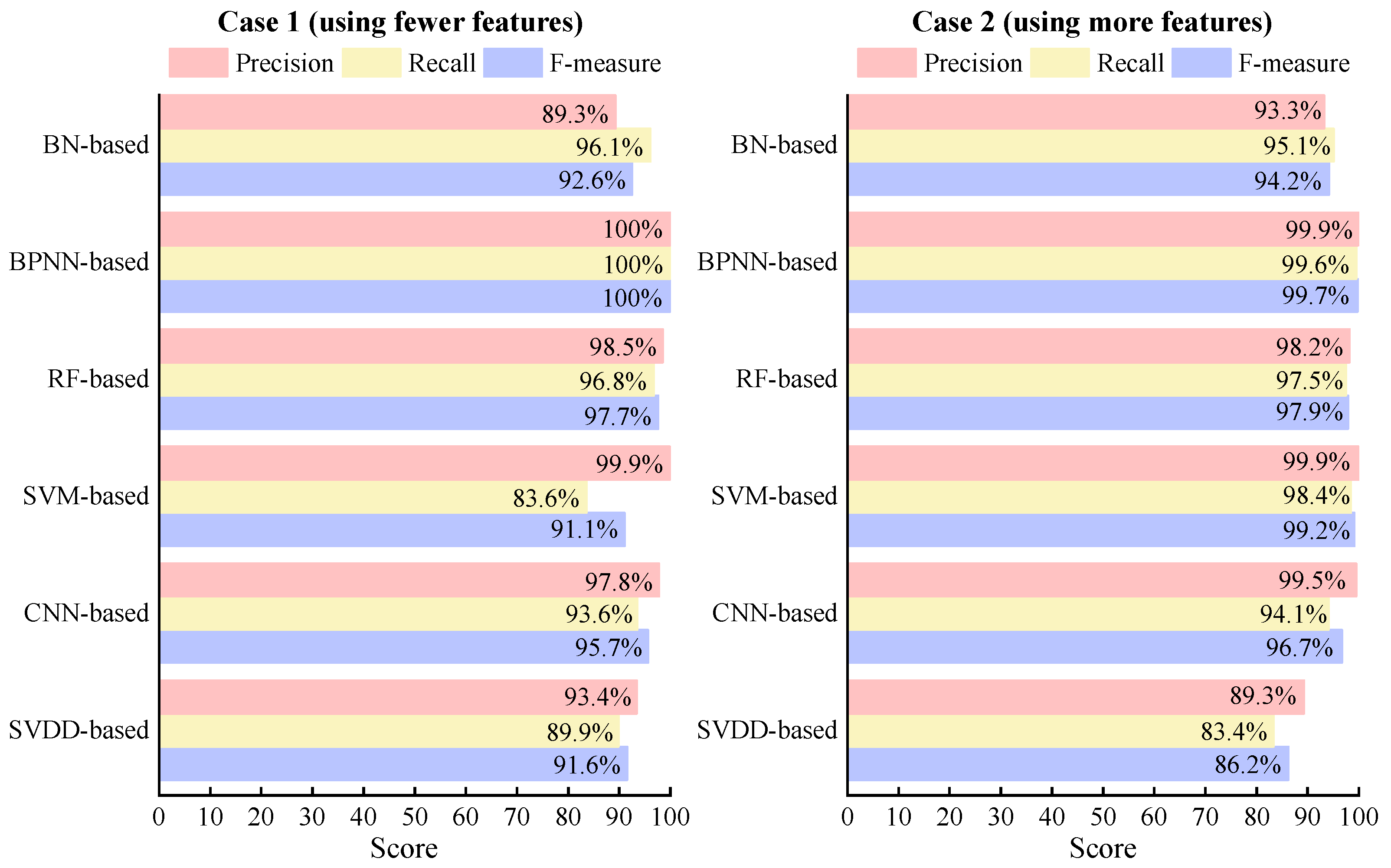
3.1. Fault Detection Results Using Foundational Models

The fault detection performance of the six foundational data-driven methods is evaluated using the normal sample data from the testing dataset. The evaluation results, represented by accuracy, are presented in Figure 3. It is worth highlighting that the definitions and computation methods for fault detection accuracy and fault diagnosis accuracy differ. Fault detection accuracy assesses the ability to correctly identify normal samples and is calculated as the ratio of correctly identified normal samples to the total number of normal samples. Conversely, fault diagnosis accuracy evaluates the proportion of correctly identified samples across all classes.

Considering both Case 1 (using fewer features) and Case 2 (using more features), under the constraint of using only features commonly available in the field, the BN-, BPNN-, RF-, and SVM-based methods achieve excellent fault detection performance, with fault detection accuracy exceeding 94%. Although the fault detection accuracy of CNN- and SVDD-based methods is lower, they still surpass 80%. These results indicate that the features commonly available in the field are sufficient to achieve an acceptable fault detection performance. However, there is still room for further improvement.

By comparing the fault detection performance under Case 1 and Case 2, it is evident that using different numbers of features has varying effects on the fault detection performance of each method. Indeed, Case 2 includes all the features from Case 1 as well as additional computed features. Clearly, there is some degree of information redundancy in the features of Case 2. Nevertheless, the results demonstrate that this redundancy negatively impacts the fault detection performance of certain methods (e.g., BN, BPNN, and RF), while positively affecting the fault detection performance of other methods (e.g., SVM, CNN, and SVDD). In detail, compared with Case 1, under Case 2, the fault detection accuracies of the BN-, BPNN-, and RF-based methods decrease by 1.0%, 0.5%, and 1.3%, respectively. However, the fault detection accuracies of the SVM-, CNN-, and SVDD-based methods increase by 1.8%, 5.3%, and 3.0%, respectively. The observation that information redundancy within the feature set impacts the fault detection performance of various methods differently suggests that each method may necessitate a unique and optimal feature combination to achieve peak performance. Hence, it is recommended to select the optimal feature combination individually for each method.

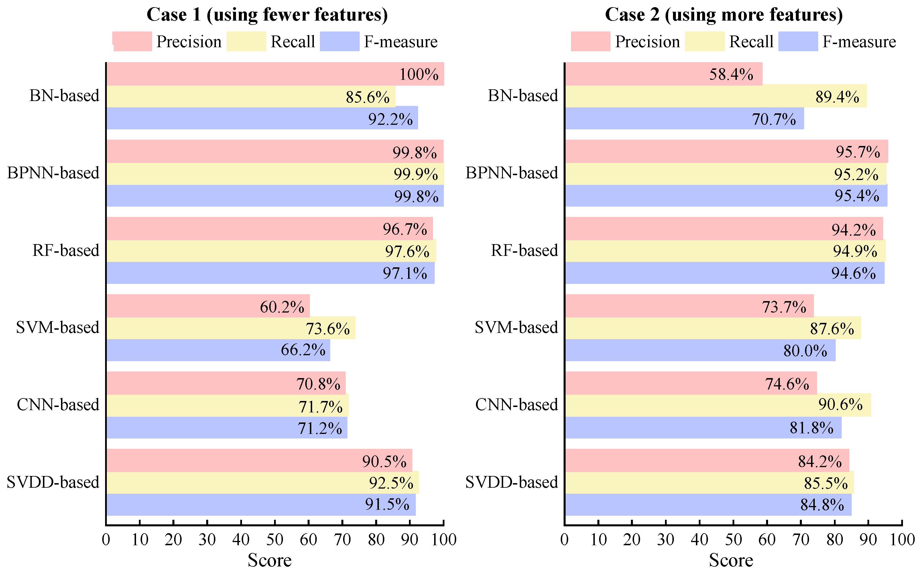
3.2. Fault Diagnosis Results Using Foundational Models

The fault diagnosis performance of the six foundational data-driven methods is evaluated using the sample data of each fault type from the testing dataset. The evaluation results are as follows.

3.2.1. Overall Fault Diagnosis Performance

The diagnostic results for the seven typical faults using the six foundational FDD methods under Case 1 and Case 2 are represented by the confusion matrices shown in Figure 4, Figure 5, Figure 6, Figure 7, Figure 8 and Figure 9. Based on these confusion matrices, the overall diagnostic accuracies are calculated and displayed in Figure 10.

Taking into account both Case 1 and Case 2, and using only features commonly available in the field, the BPNN-, RF-, CNN- and SVDD-based methods achieve excellent fault diagnosis performance, with fault diagnosis accuracy exceeding 90%. The BN- and SVM-based methods show lower fault diagnostic accuracy but still exceed 80%. Similar to fault detection, the features commonly available in the field are sufficient to achieve an acceptable fault diagnosis performance. However, there is still room for further improvement.

Indeed, by comparing the fault diagnosis performance under Case 1 and Case 2, it can be observed that the number of features used has different impacts on the fault diagnosis performance for different methods. For instance, when moving from Case 1 to Case 2, the fault diagnosis accuracies of the BPNN-, RF-, and SVDD-based methods decrease by 2.6%, 0.7%, and 4.3%, respectively. On the other hand, the fault diagnosis accuracies of the BN-, SVM-, and CNN-based methods increase by 2.5%, 5.5%, and 7.5%, respectively. Similar to fault detection, the redundant information in the features of Case 2 negatively impacts the fault diagnosis performance of certain methods, such as BPNN, RF, and SVDD. However, it has a positive impact on the fault diagnosis performance of other methods, including BN, SVM, and CNN. This finding suggests that each method may require a unique and optimal feature combination to achieve the best fault diagnosis performance. Therefore, it is also advisable to select the optimal feature combination individually for each method when it comes to diagnosing faults.

3.2.2. Individual Fault Diagnosis Performance

The overall diagnostic accuracy provides an overview of the diagnostic performance, but it may not capture the individual diagnostic differences. To further analyze the diagnostic results, precision, recall and F-measure are calculated based on the confusion matrices, and the results are presented in Figure 11, Figure 12, Figure 13, Figure 14, Figure 15, Figure 16 and Figure 17.

A summary of the individual diagnostic results is as follows:

(1)

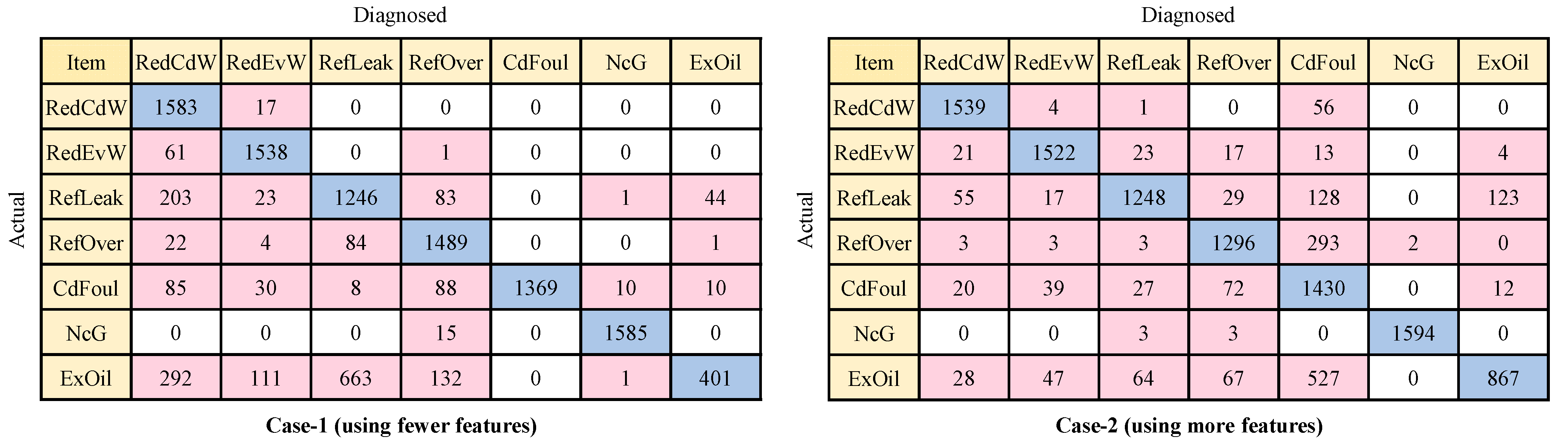
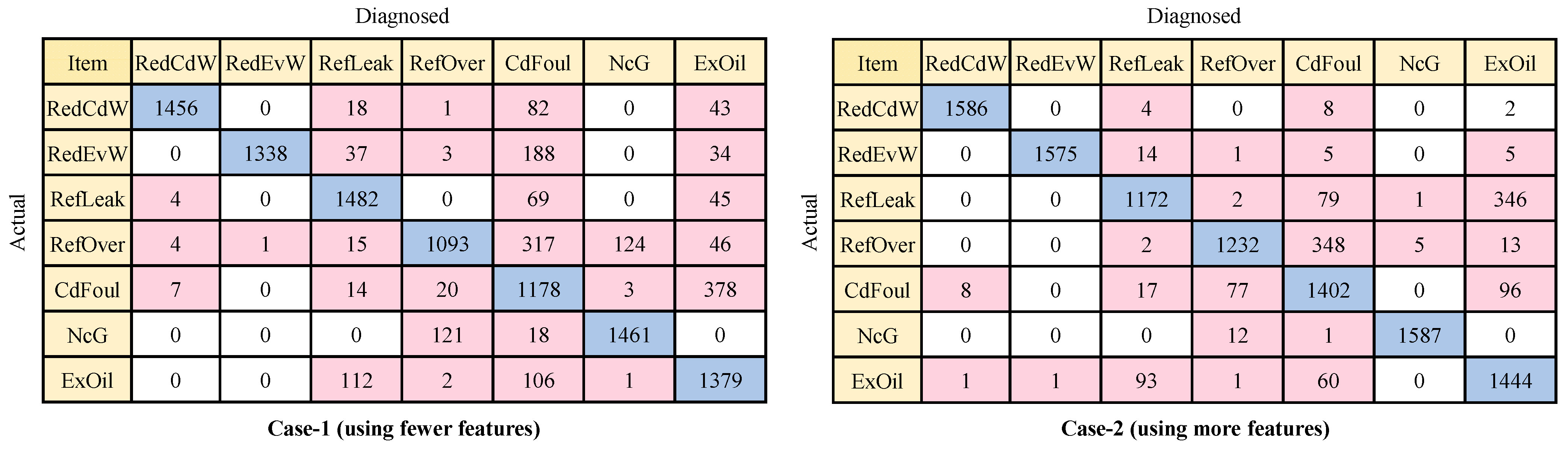
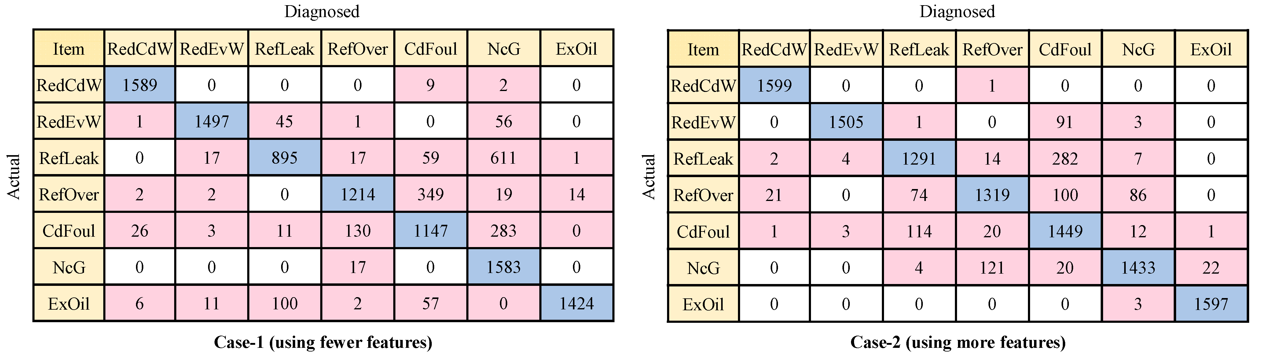
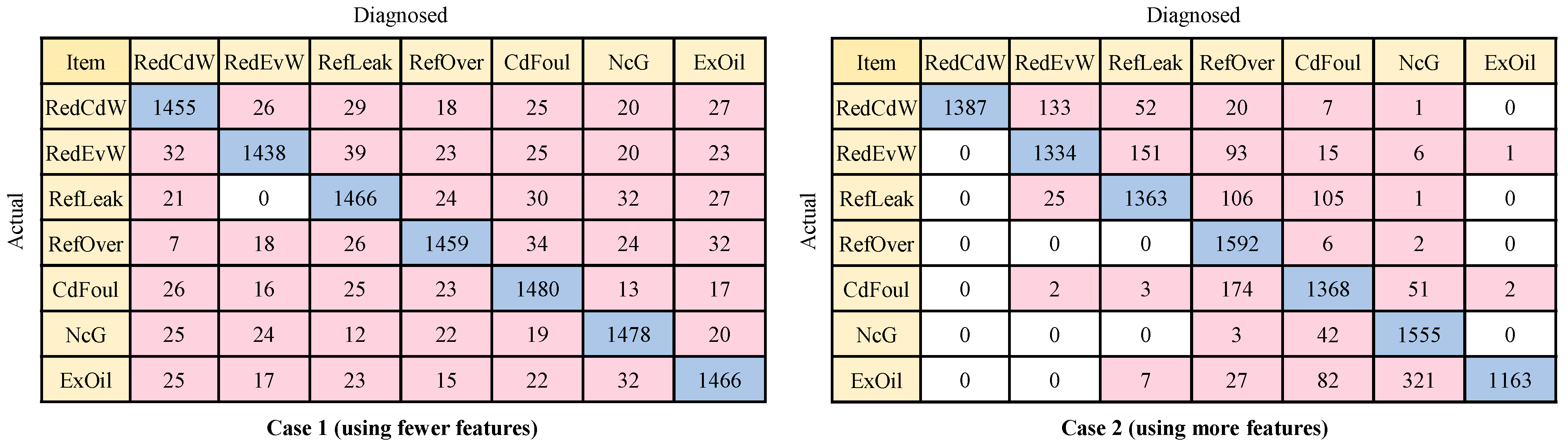
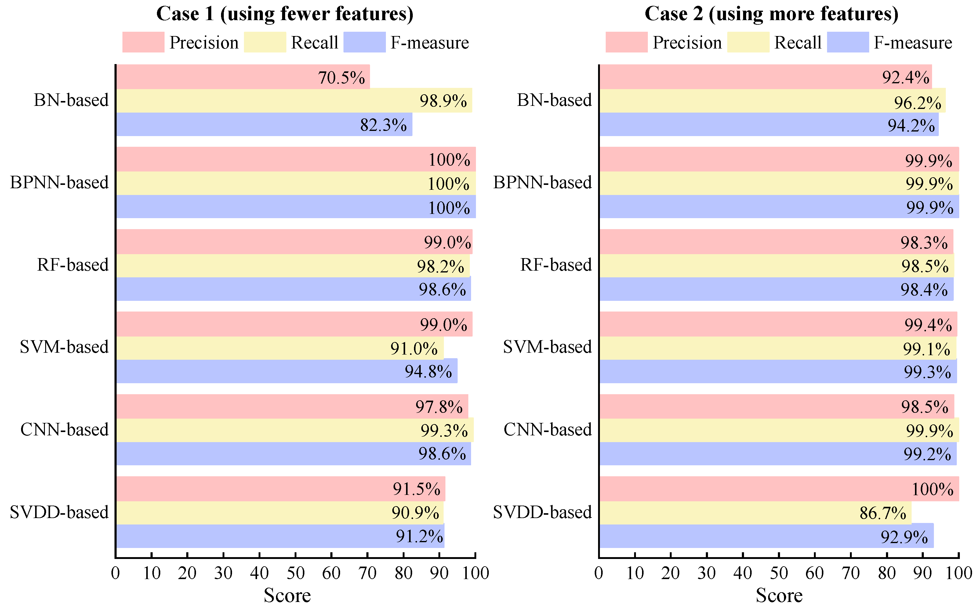
When utilizing only the features obtainable from field sensors, different data-driven methods yield diverse diagnostic results for different fault types. Considering both Case 1 and Case 2, almost all foundational FDD methods achieve F-measures over 80% for all seven faults. However, only a few foundational FDD methods achieve F-measures over 90% for all seven faults. This suggests that the features available in the field are feasible to obtain acceptable diagnostic performance for the seven typical faults but may not be sufficient to achieve excellent diagnostic performance. Further improvement might require additional features to enhance the diagnostic capabilities;

(2)

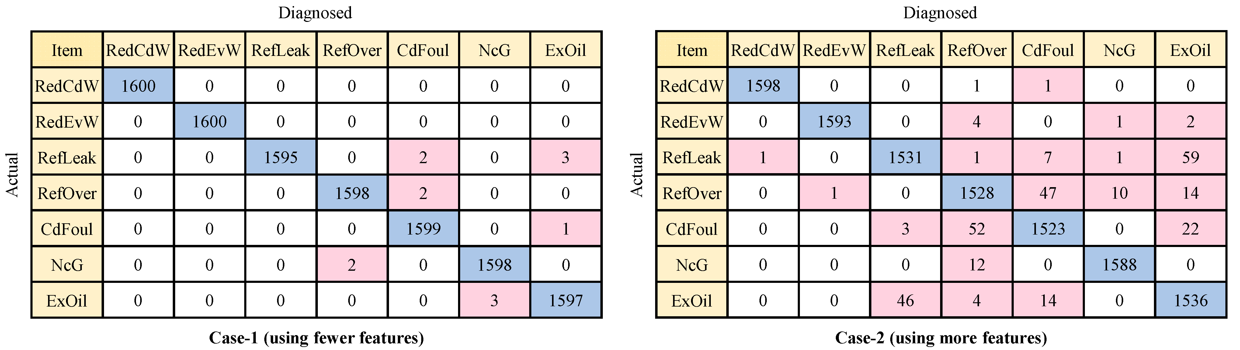
Based on the number of FDD methods with F-measures over 90% for each fault, when using only features obtainable from field sensors, RedCdW, RedEvW, and NcG are the easiest faults to diagnose. All six foundational FDD methods achieve F-measures over 90% for these three faults. RefLeak, CdFoul, and ExOil are relatively easier to diagnose, with five or four foundational methods achieving F-measures over 90% for each of them. On the other hand, RefOver is the most challenging fault to diagnose, with only three foundational methods achieving F-measures over 90%;

(3)

Upon analyzing the confusion matrix, it is evident that there is significant confusion between RefOver and CdFoul faults. For instance, for BN-, SVM-, and CNN-based methods, 293, 348, and 349 RefOver samples, respectively, were misdiagnosed as CdFoul. According to the experimental results [45], certain features used, such as $P_{in}$, $PRC$, and $TCA$, exhibit similar changing trends when RefOver and CdFoul faults occur, and this similarity has a notable negative impact on the BN-, SVM-, and CNN-based methods. Therefore, it is necessary to supplement additional features for effective diagnosis of RefOver;

(4)

Further analysis reveals that when using the same feature combination, such as using features from either Case 1 or Case 2, the six foundational data-driven methods achieve different results in fault detection and diagnosis. Some methods show better FDD performance than the others. For example, in Case 1, the fault detection accuracy of the BN-based method is 18.5% higher than that of the CNN-based method, and the fault diagnosis accuracy of the BPNN-based method is 17.6% higher than that of the BN-based method. This indicates that different methods may have different optimal feature combinations to achieve the best FDD performance. This also highlights the necessity of feature selection for each method separately. Therefore, it is advisable to individually choose the optimal feature combination for each FDD method.

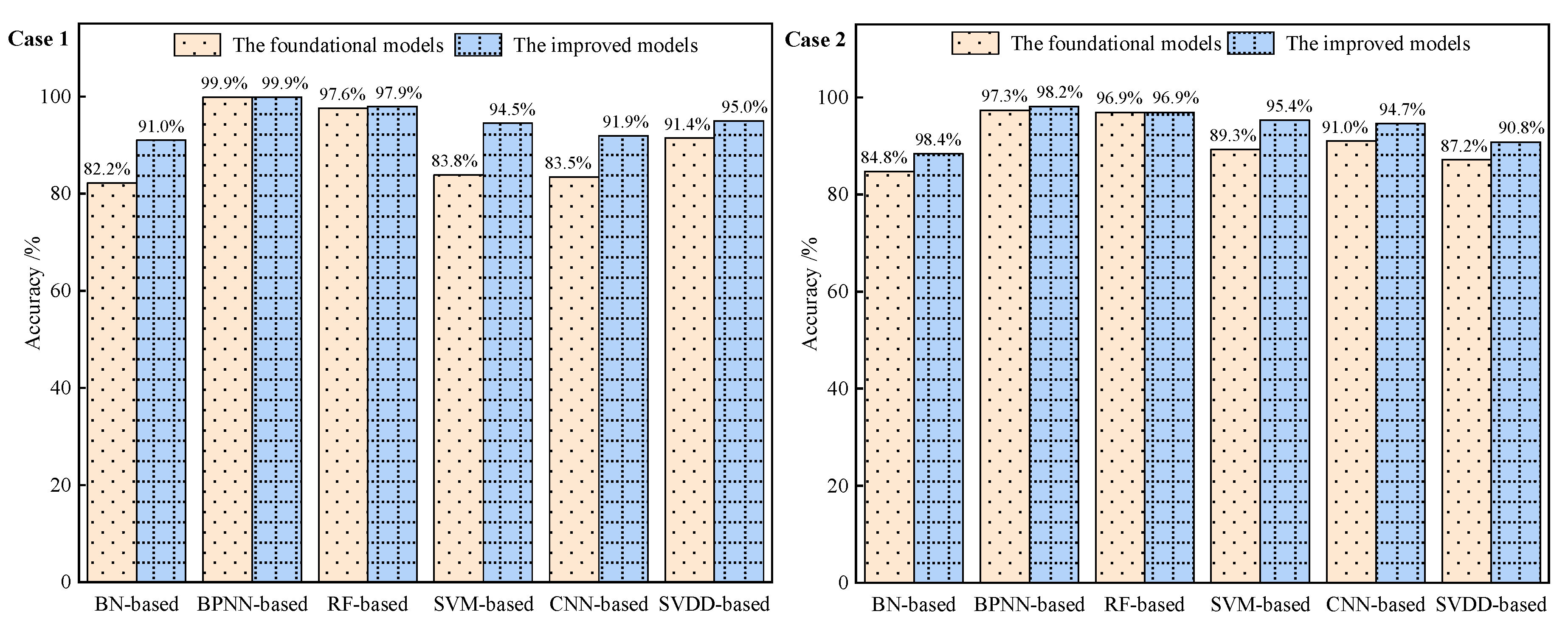
3.3. Fault Diagnosis Results Using Improved Models

To assess the optimal performance achievable by improved data-driven methods, enhanced versions of BPNN, CNN, SVM, SVDD, BN, and RF models were employed in evaluating the selected features. These foundational models are improved through the use of a genetic algorithm to optimize their parameters. Specifically, for SVM and SVDD models, the genetic algorithm was utilized to optimize the penalty constant and width of the Gaussian. In the case of BN, the genetic algorithm was applied to optimize the Gaussian parameters when the state of the parent node is false. Additionally, for BPNN and CNN, the genetic algorithm was employed to optimize the learning rate, as well as the numbers of convolutional and pooling layers, respectively.

The diagnostic accuracies of the improved models and their comparison with the foundational models are illustrated in Figure 18. The results demonstrate that after model optimization, all six models exhibit improved diagnostic performance, with the maximum enhancement reaching 10.7% (SVM in Case 1). In situations where only features commonly available in the field are considered, the improved models achieve diagnostic accuracies exceeding 90%. However, it is important to note that model optimization comes at a substantial time cost. The training time for the improved models were calculated using the training sets. For training the models, all samples from the training set were utilized. Results regarding the time cost of model training are presented in

Table 3. The time cost of the model training for the foundational and improved models under Case 1 and Case 2.

Case	Models	BN-Based	BPNN-Based	RF-Based	SVN-Based	CNN-Based	SVDD-Based
Case 1	The foundational models	344.2 s	344.2 s	344.2 s	344.2 s	344.2 s	344.2 s
	The improved models	2019.4 s	1749.3 s	1321.2 s	1927.3 s	1141.4 s	1582.6 s
Case 2	The foundational models	382.4 s	452.8 s	139.1 s	316.5 s	315.4 s	272.4 s
	The improved models	2346.9 s	2079.3 s	1658.6 s	2467.5 s	1352.1 s	2049.5 s

Note: Calculation time was evaluated in MATLAB 2018b environment installed on a computer with Intel Core i9-10900K (3.70 GHz) CPU and 16 GB of memory.

. The compu tational outcomes indicate that, compared to the training time of the foundational models before optimization, the training time for the improved models significantly increases, with an increase ranging from 5 to 11 times. This increase in training time may represent the cost of improving diagnostic performance.

3.4. Discussions

Existing studies typically aim for optimal diagnostic performance during feature selection, disregarding the practical status of on-site sensor installations. This often leads to the selection of features challenging to obtain from on-site sensors, escalating the cost of implementing diagnostic models in real-world applications. Such limitations impede practical use, particularly in on-site scenarios with restricted or no budget for additional sensors. This paper addresses the practical constraint of limited on-site sensor installations and specifically delves into the best achievable diagnostic performance using only features obtained from on-site sensors. The study focuses on typical data-driven diagnostic methods and their improved models. According to the evaluation results, features available in the field are adequate for achieving acceptable diagnostic performance (e.g., accuracies or F-measures exceeding 80%) for the seven typical faults but may fall short for achieving excellent diagnostic performance (e.g., accuracies or F-measures exceeding 90%). Additional sensors (features) might be necessary to enhance diagnostic capabilities.

Furthermore, under the constraint of using only on-site sensors, this paper identifies which faults can achieve excellent diagnostic performance and which cannot. For example, RedCdW, RedEvW, and NcG are the faults most easily diagnosed with excellent performance. Conversely, RefOver is the most challenging fault to achieve excellent diagnostic performance, with F-measures over 90%. While the improved models lead to better diagnostic performance, they come with increased computational costs and longer training times. This implies that on-site hardware needs upgrading to meet the additional computational demands, incurring certain cost increments. Such changes are generally met with reluctance from users/manufacturers. These results offer valuable guidance for users/manufacturers. For instance, if users/manufacturers lack the budget to add sensors, they can rely on the diagnostic results for RedCdW, RedEvW, and NcG with a high level of confidence. If budget constraints allow for only a limited addition of sensors, priority should be given to addressing the RefOver fault.

This paper exclusively presents the diagnostic performance attainable by typical foundational and their enhanced data-driven methods under the constraint of using only on-site sensors. Further research is warranted in two key aspects: (1) exploring the diagnostic performance of more advanced diagnostic models under the constraint of using only on-site sensors; (2) addressing the question of which sensors need to be supplemented and the strategy for supplementation to further enhance diagnostic performance. These areas will be the focal points of future research.

4. Conclusions

Under the constraints of only using the features obtained through field-installed sensors, the FDD performance of current mainstream data-driven methods is evaluated to shed light on whether it is still be effective to obtain an expected performance. The main conclusions are as follows:

(1)

For these foundational models, considering the overall FDD performance, using features commonly available in the field is adequate to achieve acceptable FDD performance, such as accuracies or F-measures exceeding 80%. However, it falls short of obtaining excellent FDD performance, defined as accuracies or F-measures exceeding 90%. This conclusion provides valuable information for users/manufacturers with limited or no budget regarding the best diagnostic performance achievable using the current mainstream data-driven methods;

(2)

While the improved models result in enhanced diagnostic performance, they are accompanied by increased computational costs and longer training times. The findings indicate that after model optimization, all six models exhibited improved diagnostic performance, with the maximum improvement reaching 10.7% (SVM in Case 1). However, it is important to note that the training time significantly increased, ranging from 5 to 11 times;

(3)

Not all typical chiller faults require additional features to achieve excellent FDD performance. Based on the number of FDD methods with F-measures exceeding 90%, the faults of RedCdW, RedEvW, and NcG are the easiest to diagnose even without supplementing additional features. However, the fault of RefOver is the most challenging, with only three foundational methods achieving F-measures over 90%. The conclusion emphasizes the necessity of supplementing additional features for a more precise diagnosis of RefOver, providing valuable guidance for users/manu facturers aiming to enhance FDD performance;

(4)

Moreover, each method may require a distinct optimal feature combination to attain the best FDD performance. The impact of information redundancy within the feature set varies among different methods, with effects that can be either negative or positive. Consequently, it is crucial to individually choose the optimal feature combination for each method.

References

1. Nalley, S. Annual Energy Outlook 2021; Energy Information Administration: Washington, DC, USA, 2021.
2. Building Energy Conservation Research Center of Tsinghua University. China Building Energy Conservation Annual Development Report; China Building Industry Press: Beijing, China, 2021. [Google Scholar]
3. Wang, Z.; Wang, L.; Ma, A.; Liang, K.; Song, Z.; Feng, L. Performance evaluation of ground water-source heat pump system with a fresh air pre-conditioner using ground water. Energy Convers. Manag. 2019, 188, 250–261. [Google Scholar] [CrossRef]
4. Katipamula, S.; Brambley, M.R. Review Article: Methods for Fault Detection, Diagnostics, and Prognostics for Building Systems—A Review, Part I. HVACR Res. 2005, 11, 3–25. [Google Scholar] [CrossRef]
5. Zhao, Y.; Li, T.; Zhang, X.; Zhang, C. Artificial intelligence-based fault detection and diagnosis methods for building energy systems: Advantages, challenges and the future. Renew. Sustain. Energy Rev. 2019, 109, 85–101. [Google Scholar] [CrossRef]
6. Mirnaghi, M.S.; Haghighat, F. Fault detection and diagnosis of large-scale HVAC systems in buildings using data-driven methods: A comprehensive review. Energy Build. 2020, 229, 110492. [Google Scholar] [CrossRef]
7. Wei, Y.; Zhang, X.; Shi, Y.; Xia, L.; Pan, S.; Wu, J.; Han, M.; Zhao, X. A review of data-driven approaches for prediction and classification of building energy consumption. Renew. Sustain. Energy Rev. 2018, 82, 1027–1047. [Google Scholar] [CrossRef]
8. Kim, W.; Katipamula, S. A review of fault detection and diagnostics methods for building systems. Sci. Technol. Built Environ. 2018, 24, 3–21. [Google Scholar] [CrossRef]
9. Shi, Z.; O’Brien, W. Development and implementation of automated fault detection and diagnostics for building systems: A review. Autom. Constr. 2019, 104, 215–229. [Google Scholar] [CrossRef]
10. Chen, J.; Zhang, L.; Li, Y.; Shi, Y.; Gao, X.; Hu, Y. A review of computing-based automated fault detection and diagnosis of heating, ventilation and air conditioning systems. Renew. Sustain. Energy Rev. 2022, 161, 112395. [Google Scholar] [CrossRef]
11. Chen, Z.; O’Neill, Z.; Wen, J.; Pradhan, O.; Yang, T.; Lu, X.; Lin, G.; Miyata, S.; Lee, S.; Shen, C.; et al. A review of data-driven fault detection and diagnostics for building HVAC systems. Appl. Energy 2023, 339, 121030. [Google Scholar] [CrossRef]
12. Borda, D.; Bergagio, M.; Amerio, M.; Masoero, M.C.; Borchiellini, R.; Papurello, D. Development of Anomaly Detectors for HVAC Systems Using Machine Learning. Processes 2023, 11, 535. [Google Scholar] [CrossRef]
13. Gao, Y.; Miyata, S.; Akashi, Y. Automated fault detection and diagnosis of chiller water plants based on convolutional neural network and knowledge distillation. Build. Environ. 2023, 245, 110885. [Google Scholar] [CrossRef]
14. Gao, J.; Han, H.; Ren, Z.; Fan, Y. Fault diagnosis for building chillers based on data self-production and deep convolutional neural network. J. Build. Eng. 2021, 34, 102043. [Google Scholar] [CrossRef]
15. Han, H.; Zhang, Z.; Cui, X.; Meng, Q. Ensemble learning with member optimization for fault diagnosis of a building energy system. Energy Build. 2020, 226, 110351. [Google Scholar] [CrossRef]
16. Fan, Y.; Cui, X.; Han, H.; Lu, H. Feasibility and Improvement of Fault Detection and Diagnosis Based on Factory-Installed Sensors for Chillers. Appl. Therm. Eng. 2020, 164, 114506. [Google Scholar] [CrossRef]
17. Ebrahimifakhar, A.; Kabirikopaei, A.; Yuill, D. Data-driven fault detection and diagnosis for packaged rooftop units using statistical machine learning classification methods. Energy Build. 2020, 225, 110318. [Google Scholar] [CrossRef]
18. van de Sand, R.; Corasaniti, S.; Reiff-Stephan, J. Data-driven fault diagnosis for heterogeneous chillers using domain adaptation techniques. Control. Eng. Pract. 2021, 112, 104815. [Google Scholar] [CrossRef]
19. Zhao, Y.; Xiao, F.; Wen, J.; Lu, Y.; Wang, S. A robust pattern recognition-based fault detection and diagnosis (FDD) method for chillers. HvacR Res. 2014, 20, 798–809. [Google Scholar] [CrossRef]
20. Chen, K.; Wang, Z.; Gu, X.; Wang, Z. Multicondition operation fault detection for chillers based on global density-weighted support vector data description. Appl. Soft Comput. 2021, 112, 107795. [Google Scholar] [CrossRef]
21. Zhang, C.; Peng, K.; Dong, J. An incipient fault detection and self-learning identification method based on robust SVDD and RBM-PNN. J. Process Control. 2020, 85, 173–183. [Google Scholar] [CrossRef]
22. Wang, Z.; Liang, B.; Guo, J.J.; Wang, L.; Tan, Y.; Li, X. Fault diagnosis based on residual–knowledge–data jointly driven method for chillers. Eng. Appl. Artif. Intell. 2023, 125, 106768. [Google Scholar] [CrossRef]
23. Wang, Z.; Liang, B.; Guo, J.J.; Wang, L.; Tan, Y.; Li, X.; Zhou, S. Fault Diagnosis Based on Fusion of Residuals and Data for Chillers. Processes 2023, 11, 2323. [Google Scholar] [CrossRef]
24. Ng, K.H.; Yik, F.W.H.; Lee, P.; Lee, K.; Chan, D. Bayesian Method for HVAC Plant Sensor Fault Detection and Diagnosis. Energy Build. 2020, 228, 110476. [Google Scholar] [CrossRef]
25. Li, T.; Zhao, Y.; Zhang, C.; Luo, J.; Zhang, X. A knowledge-guided and data-driven method for building HVAC systems fault diagnosis. Build. Environ. 2021, 198, 107850. [Google Scholar] [CrossRef]
26. Liu, Z.; Huang, Z.; Wang, J.; Yue, C.; Yoon, S. A novel fault diagnosis and self-calibration method for air-handling units using Bayesian Inference and virtual sensing. Energy Build. 2021, 250, 111293. [Google Scholar] [CrossRef]
27. Li, P.; Anduv, B.; Zhu, X.; Jin, X.; Du, Z. Across working conditions fault diagnosis for chillers based on IoT intelligent agent with deep learning model. Energy Build. 2022, 268, 112188. [Google Scholar] [CrossRef]
28. Choi, Y.; Yong, S. Autoencoder-driven fault detection and diagnosis in building automation systems: Residual-based and latent space-based approaches. Build. Environ. 2021, 203, 108066. [Google Scholar] [CrossRef]
29. Yoo, Y.-J. Fault Detection Method Using Multi-mode Principal Component Analysis Based on Gaussian Mixture Model for Sewage Source Heat Pump System. Int. J. Control. Autom. Syst. 2019, 17, 2125–2134. [Google Scholar] [CrossRef]
30. Zhang, H.; Chen, H.; Guo, Y.; Wang, J.; Li, G.; Shen, L. Sensor fault detection and diagnosis for a water source heat pump air-conditioning system based on PCA and preprocessed by combined clustering. Appl. Therm. Eng. 2019, 160, 114098. [Google Scholar] [CrossRef]
31. Zhang, C.; Xue, X.; Zhao, Y.; Zhang, X.; Li, T. An improved association rule mining-based method for revealing operational problems of building heating, ventilation and air conditioning (HVAC) systems. Appl. Energy 2019, 253, 113492. [Google Scholar] [CrossRef]
32. Guo, Y.; Liu, J.; Liu, C.; Zhu, J.; Lu, J.; Li, Y. Operation Pattern Recognition of the Refrigeration, Heating and Hot Water Combined Air-Conditioning System in Building Based on Clustering Method. Processes 2023, 11, 812. [Google Scholar] [CrossRef]
33. Chen, Y.; Zhang, D.; Yan, R. Domain adaptation networks with parameter-free adaptively rectified linear units for fault diagnosis under variable operating conditions. IEEE Trans. Neural Netw. Learn. Syst. 2023. [Google Scholar] [CrossRef]
34. Chen, Y.; Zhang, D.; Zhang, H.; Wang, Q.-G. Dual-path mixed-domain residual threshold networks for bearing fault diagnosis. IEEE Trans. Ind. Electron. 2022, 69, 13462–13472. [Google Scholar] [CrossRef]
35. Wang, D.; Yang, J.; Liu, X.; Yang, Q.; Wang, Q. Wavelet neural network approach for fault diagnosis to a chemical reactor. In Proceedings of the 2006 6th World Congress on Intelligent Control and Automation, Dalian, China, 21–23 June 2006; Volume 2, pp. 5764–5768. [Google Scholar]
36. Comstock, M.C.; Braun, J.E.; Groll, E.A. The Sensitivity of Chiller Performance to Common Faults. HVACR Res. 2001, 7, 263–279. [Google Scholar] [CrossRef]
37. Zhou, Q.; Wang, S.; Xiao, F. A Novel Strategy for the Fault Detection and Diagnosis of Centrifugal Chiller Systems. HVACR Res. 2009, 15, 57–75. [Google Scholar] [CrossRef]
38. Bai, X.; Zhang, M.; Jin, Z.; You, Y.; Liang, C. Fault detection and diagnosis for Chiller based on Feature-recognition model and Kernel Discriminant Analysis. Sustain. Cities Soc. 2022, 79, 103708. [Google Scholar] [CrossRef]
39. Zhang, L.; Frank, S.; Kim, J.; Jin, X.; Leach, M. A systematic feature extraction and selection framework for data-driven whole-building automated fault detection and diagnostics in commercial buildings. Build. Environ. 2020, 186, 107338. [Google Scholar] [CrossRef]
40. Han, H.; Gu, B.; Wang, T.; Li, Z. Important sensors for chiller fault detection and diagnosis (FDD) from the perspective of feature selection and machine learning. Int. J. Refrig. 2011, 34, 586–599. [Google Scholar] [CrossRef]
41. Gao, Y.; Han, H.; Ren, Z.X.; Gao, J.; Jiang, S.; Yang, Y. Comprehensive Study on Sensitive Parameters for Chiller Fault Diagnosis. Energy Build. 2021, 251, 111318. [Google Scholar] [CrossRef]
42. Yan, K.; Ma, L.; Dai, Y.; Shen, W.; Ji, Z.; Xie, D. Cost-sensitive and Sequential Feature Selection for Chiller Fault Detection and Diagnosis. Int. J. Refrig. 2017, 86, 401–409. [Google Scholar] [CrossRef]
43. Wang, Z.; Wang, Z.; Gu, X.; He, S.; Yan, Z. Feature selection based on Bayesian network for chiller fault diagnosis from the perspective of field applications. Appl. Therm. Eng. 2018, 129, 674–683. [Google Scholar] [CrossRef]
44. Zhao, X.; Yang, M.; Li, H. Field implementation and evaluation of a decoupling-based fault detection and diagnostic method for chillers. Energy Build. 2014, 72, 419–443. [Google Scholar] [CrossRef]
45. Comstock, M.C.; Braun, J.E. Development of Analysis Tools for the Evaluation of Fault Detection and Diagnostics for Chillers; ASHRAE Research Project 1043-RP, HL 99-20, Report #4036-3; Purdue University: West Lafayette, IN, USA, 1999. [Google Scholar]
46. Rossi, T.M. Detection, Diagnosis, and Evaluation of Fault in Vapor Compressor Cycle Equipment. Ph.D. Thesis, Purdue University, West Lafayette, IN, USA, 1995. [Google Scholar]
47. Wang, F. The use of artificial neural networks in a geographical information system for agricultural land-suitability assessment. Environ. Plan. A 1994, 26, 265–284. [Google Scholar] [CrossRef]
Figure 1. FDD framework of the one-class classification-based methods.
Processes 11 03299 g001
Figure 2. FDD framework of the multi-class classification-based methods.
Processes 11 03299 g002
Figure 3. Fault detection accuracies of the six foundational data-driven methods under Case 1 and Case 2.
Processes 11 03299 g003
Figure 4. Confusion matrix of the BN-based method under Case 1 and Case 2.
Processes 11 03299 g004
Figure 5. Confusion matrix of the BPNN-based method under Case 1 and Case 2.
Processes 11 03299 g005
Figure 6. Confusion matrix of the RF-based method under Case 1 and Case 2.
Processes 11 03299 g006
Figure 7. Confusion matrix of the SVM-based method under Case 1 and Case 2.
Processes 11 03299 g007
Figure 8. Confusion matrix of the CNN-based method under Case 1 and Case 2.
Processes 11 03299 g008
Figure 9. Confusion matrix of the SVDD-based method under Case 1 and Case 2.
Processes 11 03299 g009
Figure 10. Fault diagnosed accuracies of the six foundational data-driven methods under Case 1 and Case 2.
Processes 11 03299 g010
Figure 11. Precision, recall, and F-measure of RedCdW using the six foundational data-driven methods under Case 1 and Case 2.
Processes 11 03299 g011
Figure 12. Precision, recall, and F-measure of RedEvW using the six foundational data-driven methods under Case 1 and Case 2.
Processes 11 03299 g012
Figure 13. Precision, recall, and F-measure of RefLeak using the six foundational data-driven methods under Case 1 and Case 2.
Processes 11 03299 g013
Figure 14. Precision, recall, and F-measure of RefOver using the six foundational data-driven methods under Case 1 and Case 2.
Processes 11 03299 g014
Figure 15. Precision, recall, and F-measure of CdFoul using the six foundational data-driven methods under Case 1 and Case 2.
Processes 11 03299 g015
Figure 16. Precision, recall, and F-measure of NcG using the six foundational data-driven methods under Case 1 and Case 2.
Processes 11 03299 g016
Figure 17. Precision, recall, and F-measure of ExOil using the six foundational data-driven methods under Case 1 and Case 2.
Processes 11 03299 g017
Figure 18. The diagnostic accuracies of the improved models and their comparison with the foundational models.
Processes 11 03299 g018