Thermal, Lighting and IAQ Control System for Energy Saving and Comfort Management

Abstract

The present work proposes a simulation and control framework for home and building automation, focusing on heating, ventilating, and air conditioning processes. Control systems based on different advanced control architectures and different control policies are simulated and compared, highlighting control performances, and energy-saving results in terms of CO₂ emissions reduction. Heat, lighting, and natural ventilation phenomena were modelized through first-principles and empirical equations, obtaining a reliable and flexible simulation framework. Energy-consuming and green energy-supplying renewable sources were integrated into the framework, e.g., heat pumps, artificial lights, fresh air flow, and natural illuminance. Different control schemes are proposed, based on proportional–integral–derivative advanced control architectures and discrete event dynamic systems-based supervisors; different control specifications are included, resulting in a multi-mode control system. The specifications refer to energy savings and comfort management, while minimizing overall costs. Comfort specifications include thermal comfort, lighting comfort, and a good level of indoor air quality. Simulations on different scenarios considering various control schemes and specifications show the reliability and soundness of the simulation and control framework. The simulated control and energy performances show the potential of the proposed approach, which can provide energy-saving results greater or equal to 6 [%] (in each season) and 19 [%] (in one year) with respect to more standard approaches.

1. Introduction

Energy efficiency and energy performance maximization in buildings represent a challenge, as stated by the European Parliament in the last decade. The main objective is to reduce greenhouse gas emissions further by at least 40% by 2030 as compared with 1990, to increase the proportion of renewable energy consumed, to make energy savings in accordance with European Union level ambitions, and to improve Europe’s energy security, competitiveness, and sustainability [1,2]. An efficient and resilient building and construction sector is a fundamental requirement for zero-emission policies and clean energy transition. For example, in 2017, buildings’ construction and operations accounted for 36% of the global final energy use and nearly 40% of the energy-related carbon dioxide (CO₂) emissions [3]. In this context, programs have been introduced in the last few years, e.g., Agenda 2030 [4] at the global level and PNRR (Piano Nazionale di Ripresa e Resilienza) at the Italian level [5].

An efficient approach to reaching optimal solutions is to consider the hardware and software aspects of the buildings: hardware may refer to construction technologies and the geometry of the buildings while, software programs can exploit monitoring, modelization, control, and automation strategies [6]. Monitoring, control [7] and automation strategies [8,9] can be cross-fertilized from other areas, e.g., petrochemical and/or energy-intensive industries [10,11].

The processes which require significant energy consumption in buildings are heating, ventilating and air conditioning (HVAC), heating, ventilating, air conditioning and refrigeration (HVACR), and domestic hot water (DHW). The home and building automation (HBA) research area can cover these topics [12]. With regard to HVAC, four main factors have to be taken into account: thermal comfort, lighting comfort, a good level of indoor air quality (IAQ), and energy saving. In this context, comfort can be reached by maximizing the natural illuminance, maintaining a desirable indoor temperature, and ensuring IAQ. Conflicting objectives between comfort and energy saving must be handled [13]. In the last few years, many researchers, engineers, and practitioners have proposed monitoring, simulation, high-level optimization, and control solutions for HBA.

Monitoring and simulation solutions are proposed in [14,15,16,17,18,19]. In [14], an internet of things-based occupancy monitoring system for energy-efficient smart buildings is proposed. The occupancy monitoring is obtained through a minimally intrusive way, and data fusion techniques are developed to improve the occupancy monitoring accuracy through a multitude of sources. The use of the EnergyPlus tool is discussed in [15], analyzing how simulation can support HBA and how the deployment process of simulation-assisted building control systems can be structured. In [16], the authors accurately describe a building management system (BMS), also known as a building automation and control system (BACS), highlighting the benefits provided by the design, development and implementation of automated step response testing tools. The COVID-19 consequences on buildings’ management were analyzed in [17,18], assessing the current problems and difficulties that smart buildings face and the possible future directions of this technology. In [19], a review of machine learning algorithms able to power smart homes is provided.

High-level optimization solutions are proposed in [20,21,22,23]. In [20], the bat algorithm is applied for energy optimization in residential buildings. Three environmental parameters, namely temperature, illuminance, and air quality, are the bat algorithm’s inputs, and the optimized values of these parameters are the outputs. The error difference between the environmental parameters and the optimized parameters is the inputs of the fuzzy controllers, which return energy as an output, which in turn changes the status of the concerned actuators. In [21], to minimize the daily energy cost of HVAC and lights and maintain occupant comfort, a near-optimal strategy is proposed through a daily cost optimization problem solved by combining Lagrangian relaxation, stochastic dynamic programming, and rollout technique within a surrogate optimization framework. In [22], a real-time demand response strategy based on deep reinforcement learning is proposed as an optimal energy management strategy under the uncertainty of the residents’ behavior, outdoor temperature, and renewable generation. In [23], an energy management controller is developed for the demand-side management in smart homes. Fuzzy logic and heuristic optimization techniques for cost, energy consumption, and peak-to-average ratio reduction are used.

The high-level optimization algorithms and monitoring/simulation solutions reported previously are not in charge of the management of the real-time operation of the plants. Real-time operation of the plants can be handled through process controllers. Different HBA control solutions are present in the literature, e.g., based on standard single-input single-output (SISO) proportional–integral–derivative (PID) techniques, fuzzy logic, pole placement, model predictive control (MPC) strategy, and deep learning. Standard PID techniques are proposed in [24,25,26,27,28,29]. Classical PID control algorithms are exploited in [24] for the control of a HVAC system having two zones with different properties. The PID parameters are tuned to minimize the tracking error, but the steady-state error is not totally eliminated. In [25], a tuning strategy for discharge air temperature control of air handlers in building comfort applications is designed. The proposed method adjusts fewer gain values than other tuning algorithms, and it is tested through a standard SISO loop that manipulates a valve command for the air handler in order to track the defined setpoint for the discharge air temperature. A technique for the fast tuning of the parameters of a standard PID controller of a second-order HVAC system is proposed in [26]. A Big Bang–Big Crunch algorithm is implemented, along with the PID controller, in an FPGA device in order to achieve high tuning speed. In [27], the room temperature and humidity control systems with the conventional PID control using a fixed reset or the modified PID control using adjustable resets, which compensate for the thermal loads upset, are examined through simulations. The optimization of climate conditions in office buildings is proposed in [28] by the use of modeling and simulation tools to define the buildings’ energy demand, and the design and implementation of standard PID controls for the different control areas of the HVAC system are also proposed. In [29], the modeling, numerical simulation, and intelligent control of an expert HVAC system having two different zones with variable flow rates were performed by considering the ambient temperature. Standard decoupled SISO PID architectures are used for the control of the temperature of the two zones, and the fuzzy logic is exploited for tuning purposes.

In [30,31,32], fuzzy logic is employed for control purposes in HBA. The use of smart handheld devices, using MIT App Inventor and fuzzy control, to perform the real-time monitoring and smart control of the designed intelligent windowsill system in a smart home is proposed in [30]. A fuzzy microcontroller exploits information provided by a weather station, which measures indoor illuminance, temperature-humidity, CO₂ concentration and outdoor rain, and wind direction. The control degrees of freedom are fully or partly open to the electric curtain and electric window. Other examples of fuzzy logic implementation are reported in [31,32], pursuing lighting comfort, visual comfort, thermal comfort, and energy-saving objectives. In [33], advanced controllers based on pole placement enhanced with additional variables, namely solar radiation and external temperature, are proposed as climatic control systems. The potential of model predictive control (MPC) for enhancing building and HVAC system energy efficiency is reported in [34], highlighting problem formulation, applications, and opportunities. A recent state-of-the-art review on MPC in the HVAC field is reported in [35], focusing on energy management, energy savings, simulation software, optimization, modelization, and disturbances. In [36], the combination of predictive control and deep thermo-modernization is tackled and studied in a real-world case study: the impact of weather-forecast-based regulation on energy savings for heating in multi-family buildings is assessed. Furthermore, deep learning models, such as convolutional neural networks, are reported.

As a result of the literature review, SISO PID architectures in HBA usually provide decoupled solutions for thermal, lighting, and IAQ control. On the other hand, the main drawbacks of the other analyzed control solutions are the need for in-depth process knowledge for fuzzy logic and the need for accurate models for MPC and pole-placement solutions. The present paper proposes a simulation framework and advanced control approaches for HBA based on PID and discrete event dynamic systems (DEDS), focusing on HVAC processes. Combining different PID/DEDS advanced control architectures, a multi-mode control system is derived. The energy savings and comfort specifications are taken into account and tested through tailored simulations based on different scenarios, assessing control, and energy-saving performances. The paper aims to provide adaptable knobs for engineers, researchers, and practitioners. To the best of the authors’ knowledge, in the literature on control systems in HVAC processes, the following aspects have not been explored in depth:

• The design of flexible simulation and control frameworks that allow the modelization and simulation of different environments and the test and comparison of different controllers is not present in the literature. In the design of control systems for energy saving and comfort management in HBA, flexible frameworks can represent a significant tool for designing and prototyping optimal control solutions.
• An assessment of advanced PID control architectures for energy savings and comfort management in HBA is not present in the literature. Exploiting non-standard PID control architectures, coupled control of thermal, lighting, and IAQ subprocesses can be obtained. In this way, unexpected control margins can be detected and control performance can be improved over standard PID solutions.
• The combination of advanced PID control architectures with DEDS for energy savings and comfort management in HBA is not present in the literature. This combination can result in a significant improvement in energy savings and comfort management performances with respect to more standard control architectures.

Exploiting a multivariable approach with respect to HBA standard PID solutions, further energy savings and comfort margins can be observed. As it will be shown in the paper, the proposed approach can achieve energy-saving results greater than or equal to 6 [%] (in each season) and 19 [%] (in one year) with respect to more standard approaches.

The paper is organized as follows: Section 2 reports the material and methods, focusing on PID controllers, DEDS, and simulation/control frameworks. Section 3 reports the results and discussion, focusing on the control and energy-saving performances. The conclusions are summarized in Section 4.

2. Materials and Methods

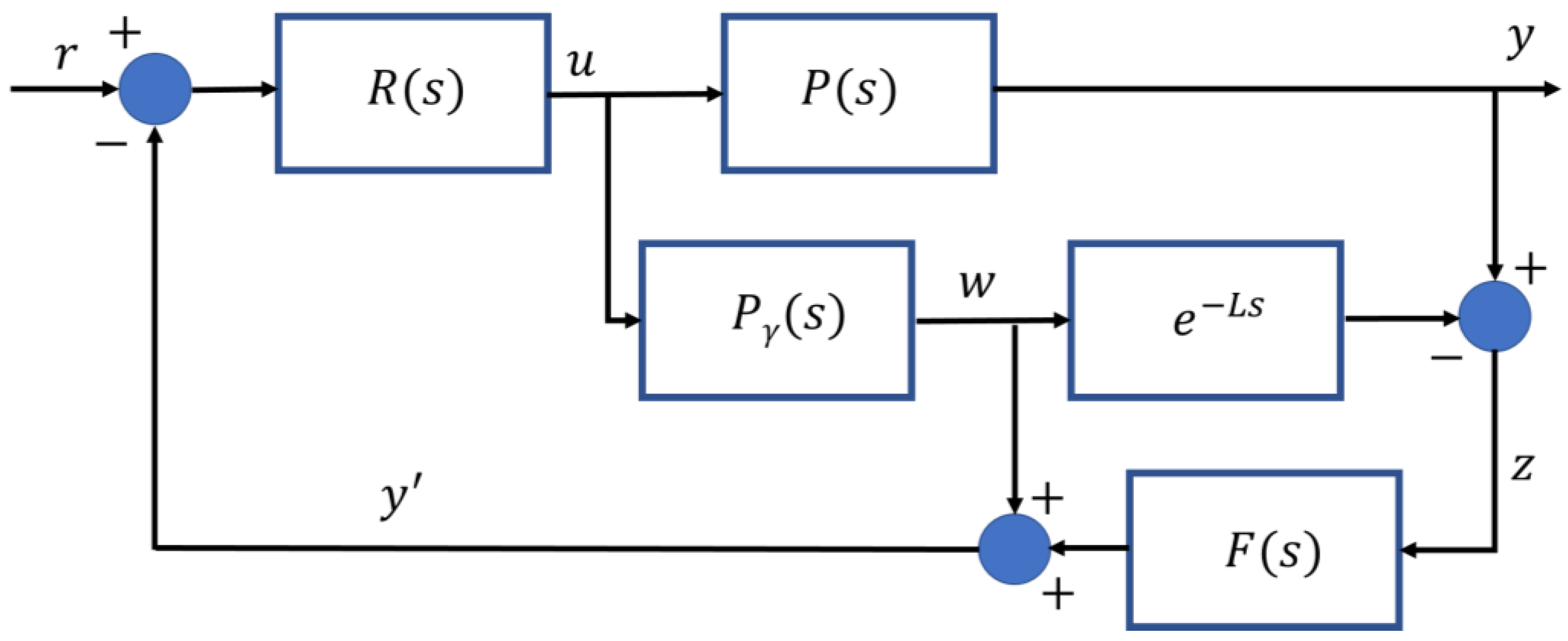
2.1. PID Control Architectures

The PID control is exploited in a large number of sectors and at different levels of the automation hierarchy. PID techniques are typically used for SISO feedback control of processes with/without dead times (or delays) [37].

PID controllers are characterized by three main components that process the control error: proportional, integral and derivative. These components are represented by the tuning parameters $K_P$, $T_I$, $T_D$ [37]. In order to efficiently control the process, the three terms have to be suitably tuned. In the literature, different tuning methods were proposed, e.g., the Ziegler-Nichols and Cohen-Coon methods. The Ziegler-Nichols frequency response and step response methods are widely used tuning methods for PID controllers [38].

The Ziegler-Nichols frequency response method (close-loop method) assumes to model the controlled process with two parameters: the ultimate gain ($K_u$) and the ultimate period ($T_u$). These parameters are determined by forcing the process through a P controller, increasing the proportional gain until the process oscillates critically. The gain yielding marginal stability is the ultimate gain, and the ultimate period is the period of oscillation in correspondence with the ultimate gain. Using the ultimate gain ($K_u$) and the ultimate period ($T_u$), the proportional, integral, and derivative gains are typically computed as in

Table 1. PID control parameters tuning (Ziegler-Nichols frequency response method) [37].

Controller	${\mathit{K}}_{\mathit{P}}$	${\mathit{T}}_{\mathit{I}}$	${\mathit{T}}_{\mathit{D}}$
P	$0.5·K_u$
PI	$0.4·K_u$	$0.8·T_u$
PID	$0.6·K_u$	$0.5·T_u$	$0.125·T_u$

[37].

The Ziegler-Nichols step response method (open-loop method) is based on an open-loop step test procedure applied to the process, hence requiring the process to be stable. The unit step response of the process is characterized by two parameters, i.e., $\alpha$ and $\tau$. These can be determined, for example, by drawing a tangent line at the inflexion point of the step response, where the slope of the step response has its maximum value. The intersections of the tangent and the coordinate axes give the parameter $\alpha$ and $\tau$ that are used to compute the proportional, integral, and derivative gains (see

Table 2. PID control parameters tuning (Ziegler-Nichols step response method) [37].

Controller	${\mathit{K}}_{\mathit{P}}$	${\mathit{T}}_{\mathit{I}}$	${\mathit{T}}_{\mathit{D}}$
P	$1/\alpha$
PI	$0.9/\alpha$	$3·\tau$
PID	$1.2/\alpha$	$2·\tau$	$\tau /2$

) [37].

As previously described, the PID technique can be exploited for the SISO control of processes with dead times (or delays). Often, industrial processes are modelized by a first-order plus deadtime (FOPDT) model. In the Laplace domain, this model is [39]:

$$y\left(s\right)=P\left(s\right)u\left(s\right)=P_{\gamma }\left(s\right)e^{-Ls}u\left(s\right)=\frac{K}{Ts+1}{e}^{-Ls}u\left(s\right)$$

(1)

where $s$ is the Laplace variable, $P\left(s\right)$ is the input-output transfer function, $P_{\gamma }\left(s\right)$ is the input-output transfer function without delay, $y$ is the output, $u$ is the input, $K$ is the gain of the process, $T$ is the time constant and $L$ is the delay. In this paper, the case where the time constant $T$ and the delay $L$ are comparable is considered, i.e., [37]:

$$0.6<\frac{L}{T}<1$$

(2)

Assuming that model (1) is sufficiently reliable, when Equation (2) holds, the Smith Predictor can be used [37]. This PID-based predictive controller overcomes the limitations of a PID controller, which exploits only feedback. A Smith Predictor architecture is reported in Figure 1. In Figure 1, $r$ is the reference to be tracked, $w$ and $z$ are intermediate variables and $y^{\prime }$ is the feedback variable. The input-output transfer function related to $y^{\prime }$ is [37]

$$y^{\prime }\left(s\right)=P_{\gamma }\left(s\right)\left(1-e^{-Ls}\right)u\left(s\right)$$

(3)

In Figure 1, $F\left(s\right)$ is a low-pass filter that allows to compensate low frequency errors. $F\left(s\right)$ can be defined as [37]:

$$F\left(s\right)=\frac{1}{0.5Ls+1}$$

(4)

In the scheme of Figure 1, $R\left(s\right)$ can be designed as a PID controller.

Different control architectures based on PID controllers were introduced by researchers, engineers, and practitioners. Examples of these architectures are cascade, split-range, valve position, and override control [37].

A cascade control structure involves two or more PID controllers in serial connection and two or more nested control loops. The manipulated variable (MV) of the master controller is connected to the setpoint of the slave controller. The advantage of the cascade control is that disturbance variables (DVs) affecting the inner loop can be compensated much more quickly in the slave (inner) loop than in the slower master (external) loop. The inner controller design is beneficial if its dynamics are faster. Cascade control requires a major effort in the tuning phase with respect to a standard PID controller. Due to the inner loop being an element within the master (external) one, it must be properly tuned before the master controller, with the master controller in manual mode. Then, the master controller should be tuned, with the inner controller in automatic mode [40].

A wide variety of process control problems are characterized by having one controlled variable (CV) and two or more MVs. The challenge from a control perspective is that there is no unique set of input values that can ensure the setpoint tracking of the CV. One of the most common ways of addressing this problem is known as split-range control. A splitter block is used to map the controller output to multiple MVs [41].

In many case studies (e.g., feedstock flow control), the synchronized use of actuators characterized by different dynamics, such as, for example, a small and a large actuation valve, can be required for accurate control over a significant operating range. An ideal solution would be to use the small valve to make fine changes and the large valve to significantly adjust the CV, differently from the split-range control, where valves are sequenced one at a time. Valve position control architecture achieves this type of regulation for the small and large valves [41].

In an override control architecture, two or more CVs share a common actuator (MV). Depending on the current process state, a decision is made on which controller is in charge of the actual manipulation of the actuator; in other words, the various controllers can override each other [37]. Figure 2 reports an override control architecture. In the case reported in Figure 2, the decision is based on a comparison of the computed MV requests of both controllers; for example, the controller that demands the higher MV value takes control of the actuator (high-pass selector). Both controllers run the entire time. This scheme can also be used in applications with more than two CVs and with low-pass selector logic.

In order to implement efficient and flexible architectures, the previous control architectures can be enriched with anti-wind-up schemes and bumpless transfer techniques to handle possible transitions between manual and automatic control modes [37].

2.2. HVAC Simulation Framework

In order to design and implement a HVAC simulation framework, first-principles, and empirical models related to an office building were combined. The considered office building is located in Ancona, Italy. The HVAC simulation framework consists of a thermal model, a lighting model and an IAQ model [42,43]. Six walls (two floors and four vertical) and two windows characterize the rectangular layout of the single office room. The considered devices are reported in Figure 3: the actuators are the rolling shutters, the windows, a light dimmer and a heat pump (with a fan coil). The measured variables are the room temperature (through a thermostat) and light (through a luxmeter). Furthermore, a weather station is considered for the measurement of the outdoor temperature, wind speed, and other parameters. Eventually, a presence sensor and IAQ sensors can be present.

Table 3. Room parameters.

Component/Device	Features	SI Measurement Unit
Room	$\left[5.0\times 4.0\times 2.7\right]$	$\left[\mathrm{m}\right]\times \left[\mathrm{m}\right]\times \left[\mathrm{m}\right]$
Wall-SW	$\left[5.0\times 2.7\right]$, Vertical	$\left[\mathrm{m}\right]\times \left[\mathrm{m}\right]$
Wall-NW	$\left[4.0\times 2.7\right]$, Vertical	$\left[\mathrm{m}\right]\times \left[\mathrm{m}\right]$
Wall-NE	[5.0 $\times$ 2.7], Vertical, (Not Exposed)	$\left[\mathrm{m}\right]\times \left[\mathrm{m}\right]$
Wall-SE	[4.0 $\times$ 2.7], Vertical, (Not Exposed)	$\left[\mathrm{m}\right]\times \left[\mathrm{m}\right]$
Wall-A	[5.0 $\times$ 4.0], Horizontal	$\left[\mathrm{m}\right]\times \left[\mathrm{m}\right]$
Wall-B	[5.0 $\times$ 4.0], Horizontal, (Not Exposed)	$\left[\mathrm{m}\right]\times \left[\mathrm{m}\right]$
Window-SW1	[2 $\times$ 1.25 $\times$ 1], Vertical	$\left[\mathrm{m}\right]\times \left[\mathrm{m}\right]\times \left[\mathrm{m}\right]$
Window-SW2	[2 $\times$ 1.25 $\times$ 1], Vertical	$\left[\mathrm{m}\right]\times \left[\mathrm{m}\right]\times \left[\mathrm{m}\right]$
Heat Pump	COP * = 2.8, Max Power = 4	$[],\left[\mathrm{kW}\right]$
Artificial Light (Dimmer)	location (2.5, 2.0, 2.4), Flux = 8900	$\left[\mathrm{m}\right],\left[\mathrm{lumen}\right]$

* COP = coefficient of performance.

reports the room parameters.

2.2.1. Thermal Model

The thermal model of the considered office room takes into account the thermal behavior of the room, which can be modelized through an energy balance equation [42] reported in (5). Six main contributions were considered in Equation (5) for the total thermal accumulation, e.g., internal heat sources ($Q_{IS}$, due to people, lamps, and motors), heat pump source ($Q_{HP}$), thermal conduction and convection exchanges through walls $\left(Q_W\right)$, thermal conduction, convection and radiation exchanges through windows ($Q_{GL\_S}$, $Q_{GL\_S\_I}$), and finally the fluid dynamic exchanges with the outside environment ($Q_{VENT}$). The thermal contributions are reported in Equations (6)–(9), while the terms involved in the Equations (5)–(9) are reported in

Table 4. Thermal model parameters (Equations (5)–(9)).

Symbol	Description	SI Measurement Unit
$Q_{IS}$	Heat supplied by internal heat sources (people, lamps, and motors)	$\left[\mathrm{W}\right]$
$Q_{HP}$	heat supplied by heat pump source	$\left[\mathrm{W}\right]$
$Q_W$	heat supplied by walls	$\left[\mathrm{W}\right]$
$Q_{GL\_S}$, $Q_{GL\_S\_I}$	heat supplied by windows	$\left[\mathrm{W}\right]$
$Q_{VENT}$	heat supplied by the outside environment	$\left[\mathrm{W}\right]$
$A_k$	$k$th wall area	$[{\mathrm{m}}^2]$
$h_{O_k}$	$k$th wall adduction coefficient	$[\mathrm{W}/({\mathrm{m}}^2·\mathrm{K})]$
$h_{Og{l}_j}$	$j$th glass adduction coefficient	$[\mathrm{W}/({\mathrm{m}}^2·\mathrm{K})]$
$F_{G\_g{l}_j}$,$F_{G\_gl\_s_j}$	solar gain coefficient ($j$th glass, $j$th glass/shutter)	$[]$
$N_j$	number of times air is exchanged through the $j$th window opening	$\left[1/\mathrm{s}\right]$
${\rho }_a$	air density	$[\mathrm{kg}/{\mathrm{m}}^3]$
$c_a$	air specific heat	$\left[\mathrm{J}/\left(\mathrm{kg}·\mathrm{K}\right)\right]$
$m_a$	room air mass	$\left[\mathrm{kg}\right]$
$V_j$	air incoming volume (fixed value) from $j$th window	$[{\mathrm{m}}^3]$
$T_{W_{k\_Lj}}$	temperature of $j$th layer of $k$th wall	$\left[\mathrm{K}\right]$
$T_{g{l}_j}$	$j$th internal temperature of glass	$\left[\mathrm{K}\right]$
$T_{gl\_s_j}$	$j$th internal temperature of glass combined with shutters	$\left[\mathrm{K}\right]$
$T_a$	room temperature	$\left[\mathrm{K}\right]$
$T_e$	outside temperature	$\left[\mathrm{K}\right]$
$A_{g{l}_j}$	$j$th glass area	$[{\mathrm{m}}^2]$
$SA{F}_j$	$j$th shutter actuation factor	$[\%]$
$I_{g{l}_j}$	$j$th glass solar thermal radiation	$[\mathrm{W}/{\mathrm{m}}^2]$

[42].

$$m_a·c_a·\frac{\partial T_a\left(t\right)}{\partial t}=Q_{IS}\left(t\right)+Q_{HP}\left(t\right)+Q_W\left(t\right)+Q_{GL\_S}\left(t\right)+Q_{GL\_S\_I}\left(t\right)+Q_{VENT}\left(t\right)$$

(5)

$$Q_W\left(t\right)={\displaystyle \sum }_{k=1}^6{A}_k·h_{O_k}·\left(T_{W_{k\_L1}}\left(t\right)-T_a\left(t\right)\right)$$

(6)

$$Q_{GL\_S}\left(t\right)={\displaystyle \sum }_{j=1}^2{A}_{g{l}_j}·h_{Og{l}_j}·\left[\left(1-SA{F}_j\left(t\right)\right)·\left(T_{g{l}_j}\left(t\right)-T_a\left(t\right)\right)+SA{F}_j\left(t\right)·\left(T_{gl\_s_j}\left(t\right)-T_a\left(t\right)\right)\right]$$

(7)

$$Q_{GL\_S\_I}\left(t\right)={\displaystyle \sum }_{j=1}^2{A}_{g{l}_j}·\left[\left(1-SA{F}_j\left(t\right)\right)·F_{G\_g{l}_j}+SA{F}_j\left(t\right)·F_{G\_gl\_s_j}\right]·I_{g{l}_j}\left(t\right)$$

(8)

$$Q_{VENT}\left(t\right)={\displaystyle \sum }_{j=1}^2{\rho }_a·c_a·N_j\left(t\right)·V_j·\left(T_e\left(t\right)-T_a\left(t\right)\right)$$

(9)

Indoor wall and glass temperatures are included in Equations (6) and (7). These terms are modelized through a dynamic multi-layer model. Figure 4 shows a multi-layer wall composed of five layers. For example, the first wall, i.e., the external wall, composed of five layers, can be modelized by Equations (10)–(14) [42] whose terms are described in

Table 5. Thermal model parameters (Equations (10)–(14)).

Symbol	Description	SI Measurement Unit
$T_{W_{k\_Lj}}$	temperature of $j$th layer of $k$th wall	$\left[\mathrm{K}\right]$
$I_{g{l}_j}$	$j$th glass solar thermal radiation	$[\mathrm{W}/{\mathrm{m}}^2]$
$T_a$	room temperature	$\left[\mathrm{K}\right]$
$T_e$	outside temperature	$\left[\mathrm{K}\right]$
$I_{W_k}$	$k$th wall solar thermal radiation	$[\mathrm{W}/{\mathrm{m}}^2]$
$A_{W_k}$	$k$th wall area	$[{\mathrm{m}}^2]$
$K_{ji}$	thermal transmittance between layers $j$ and $i$ of the wall	$[\mathrm{W}/({\mathrm{m}}^2·\mathrm{K})]$
$K_{e1}$	thermal transmittance between layer one of the wall and outdoor air	$[\mathrm{W}/({\mathrm{m}}^2·\mathrm{K})]$
$K_{5i}$	thermal transmittance between layer five of the wall and indoor air	$[\mathrm{W}/({\mathrm{m}}^2·\mathrm{K})]$
$m_i$	mass of the layer $i$ of the wall	$\left[\mathrm{kg}\right]$
$c_i$	specific heat of the layer $i$ of the wall	$\left[\mathrm{J}/\left(\mathrm{kg}·\mathrm{K}\right)\right]$
${\alpha }_e$	absorption coefficient of the wall	$[]$
$h_e$	adduction coefficient of the wall	$[\mathrm{W}/({\mathrm{m}}^2·\mathrm{K})]$
$R_{e1}$	thermal resistance of the wall	$\left[\left({\mathrm{m}}^2·\mathrm{K}\right)/\mathrm{W}\right]$
${\Gamma }_j$	internal flux parameter	$[]$
$A_{g{l}_j}$	$j$th glass area	$[{\mathrm{m}}^2]$
$Ta{u}_j$	$j$th glass transparency	$[]$
$F_j$	$j$th shutter shading factor	$[]$

.

$$\frac{\partial T_{W_k}\left(t\right)}{\partial t}=A·T_{W_k}\left(t\right)+B·u_{W_k}\left(t\right)$$

(10)

$$T_{W_k}\left(t\right)=\left[\begin{array}{c}{T}_{W_{k\_L1}}\left(t\right)\\ ⋮\\ T_{W_{k\_L5}}\left(t\right)\end{array}\right]$$

(11)

$$u_{W_k}\left(t\right)=\left[\begin{array}{c}{T}_e\left(t\right)\\ T_a\left(t\right)\\ I_{W_k}\left(t\right)\\ I_{g{l}_1} \left(t\right)\\ I_{g{l}_2} \left(t\right)\end{array}\right]$$

(12)

$$A=A_{W_k}\left[\begin{array}{ccccc}-\frac{K_{e1}+K_{12}}{m_1{c}_1}& \frac{K_{12}}{m_1{c}_1}& 0& 0& 0\\ \frac{K_{12}}{m_2{c}_2}& -\frac{K_{12}+K_{23}}{m_2{c}_2}& \frac{K_{23}}{m_2{c}_2}& 0& 0\\ 0& \frac{K_{23}}{m_3{c}_3}& -\frac{K_{23}+K_{34}}{m_3{c}_3}& \frac{K_{34}}{m_3{c}_3}& 0\\ 0& 0& \frac{K_{34}}{m_4{c}_4}& -\frac{K_{34}+K_{45}}{m_4{c}_4}& \frac{K_{45}}{m_4{c}_4}\\ 0& 0& 0& \frac{K_{34}}{m_5{c}_5}& -\frac{K_{45}+K_{5i}}{m_5{c}_5}\end{array}\right]$$

(13)

$$B=\left[\begin{array}{ccccc}{A}_{W_k}\frac{K_{e1}}{m_1{c}_1}& 0& A_{W_k}\frac{\frac{{\alpha }_e}{\left(h_e·R_{e1}\right)}}{m_1{c}_1}& 0& 0\\ 0& 0& 0& 0& 0\\ 0& 0& 0& 0& 0\\ 0& 0& 0& 0& 0\\ 0& A_{W_k}\frac{K_{5i}}{m_5{c}_5}& 0& \frac{{\Gamma }_1·A_{g{l}_1}·Ta{u}_1·F_1}{m_5{c}_5}& \frac{{\Gamma }_2·A_{g{l}_2}·Ta{u}_2·F_2}{m_5{c}_5}\end{array}\right]$$

(14)

The window’s contribution to the room’s thermal behavior is characterized by conduction, convection and radiation phenomena. Equation (7) represents conduction and convection, while Equation (8) reports the radiation contribution. In Equations (7) and (8), two sections characterize the window’s contribution (see Figure 5): the first section is related to the lower part of the glass window and takes into account only the contribution of the glass (subscript gl), while the second section takes into account the contribution of the glass coupled to the rolling shutter (subscript gl_s). These contributions are modelized separately here and not reported for brevity. The density, the thickness, and the specific heat of glass and rolling shutters characterize these contributions [44].

In order to estimate the thermal radiation related to the windows’ glass and to the walls, historical data were selected for the considered location (see Table 3). Different seasons and times of day were taken into account. These inputs, together with the disposition of the considered surfaces, were used in different algorithms, e.g., the Liu and Jordan method or the Collares-Pereira and Rabl method [45].

With regard to the outside temperature used in the thermal model, historical data were selected for the considered location (see Table 3).

The formulated thermal model can be suitably extended to different room configurations and features and to multi-room environments. For example, if a wall with more than five layers were to be considered, a number of equations (similar to Equation (10)) equal to the assumed layers’ number would result. In addition, if a multi-room environment is assumed, an equation (similar to Equation (5)) for each room must be included in the model, taking into account possible coupling effects between the different rooms.

2.2.2. Lighting Model

Artificial light and natural illuminance were considered for the designed lighting model. Different assumptions on the room/lights and room/window relative dimensions were made for the lighting model (see Table 3). The superposition principle is applied, so uniformity of the light radiation is assumed. Furthermore, extended light sources and point light sources were considered: natural light sources belong to the first category, while artificial light sources were included in the second one. Equation (15) reports the designed lighting model for a generic point of interest $P\left(x,y,z\right)$ [46,47], while

Table 6. Lighting model parameters (Equation (15)).

Symbol	Description	SI Measurement Unit
$E_a$	environment illuminance at the point of interest $P\left(x,y,z\right)$	$\left[\mathrm{Lux}\right]$
$E_{N\_D\_gl,j}$	natural diffuse illuminance on the window	$\left[\mathrm{Lux}\right]$
$E_{N\_R\_gl,j}$	natural reflection illuminance on glass	$\left[\mathrm{Lux}\right]$
$E_{NAT\_gl,j}$	natural direct illuminance on glass	$\left[\mathrm{Lux}\right]$
$C_{j,c}$,$C_{j,r}$	environmental influence of natural diffuse/reflections illuminance at the point of interest $P\left(x,y,z\right)$	$[]$
$I_L$	artificial light source luminous emission	$\left[\mathrm{cd}/\mathrm{klm}\right]$
$Lumen$	luminous flux of the artificial light source	$\left[\mathrm{lm}\right]$
$\gamma$	incidence angle of the light radiation in relation to the point of interest $P\left(x,y,z\right)$	$\left[°\mathrm{C}\right]$
$h$	distance between the point of interest and light source	$\left[\mathrm{m}\right]$
$Ta{u}_j$	$j$th glass transparency	$[]$
$V_j$	natural direct illuminance coefficient	$[]$
$A_{g{l}_j}$	$j$th glass area	$[{\mathrm{m}}^2]$
$\rho$	reflection coefficient	$[]$
${\rho }_{weighted}$	average reflection coefficient of the walls	$[]$
$su{m}_{AREA}$	total area of the reflective walls	$[{\mathrm{m}}^2]$
$E_{NAT\_gl,j}$	$j$th glass area	$[{\mathrm{m}}^2]$
$\eta$	efficiency of artificial light source	$[]$
$M$	maintenance factor	$[]$

summarizes the involved parameters.

$$\begin{gathered} E_a\left(t\right)={\displaystyle \sum }_{j=1}^2\left|C_{j,c}·E_{N\_D\_gl,j}\left(t\right)+C_{j,r}·E_{N\_R\_gl,j}\left(t\right)\right|+\frac{I_L\left(t\right)·Lumen ·1000·\cos {\left(\gamma \right)}^3}{h^2} \\ +{\displaystyle \sum }_{j=1}^2\frac{Ta{u}_j·V_j·A_{glj}·{\rho }_{weighted}}{su{m}_{AREA}·\left(1-{\rho }_{weighted}\right)}{E}_{NAT\_gl,j}\left(t\right)+\frac{Lumen·\eta ·M·\rho }{su{m}_{AREA}·\left(1-{\rho }_{weighted}\right)} \end{gathered}$$

(15)

The natural illuminance used in the lighting model was estimated. Historical data were selected for the considered location (see Table 3). Different seasons and times of day were taken into account.

The formulated lighting model can be suitably extended to different room configurations and features and to multi-room environments. For example, if different points of interest were to be considered, an equation (similar to Equation (15)) for each point of interest must be formulated. Furthermore, if more artificial light sources are present, different artificial light source contributions (similar to the second and fourth terms of Equation (15)) must be included. In addition, if more windows are present, different natural light source contributions (similar to the first and third terms of Equation (15)) have to be considered.

2.2.3. IAQ Model

The IAQ model is composed of three main sources of pollution: formaldehyde (HCHO), carbon dioxide (CO₂) and TVOC (total volatile organic compounds). The first one consists of a colorless organic compound with a highly irritating odor, used mainly in the production of wood panels and furniture, paints, and laminate. CO₂ is produced by people in sedentary work in the room. The last source of pollution, i.e., TVOC, includes different chemical compounds. The concentration of toxic waste can be evaluated in terms of the volume of pollution to the volume of standard indoor air [48].

IAQ dynamics are represented in Equations (16)–(19), while

Table 7. IAQ model parameters (Equations (16)–(19)).

Symbol	Description	SI Measurement Unit
${\mathrm{CO}}_2$	room ${\mathrm{CO}}_2$	$\left[{\mathrm{m}}^3{\mathrm{CO}}_2\right]$
$n_{people}$	number of people in the room	$[]$
$E_p$	${\mathrm{CO}}_2$ emissions for each people (sedentary)	$\left[{\mathrm{m}}^3{\mathrm{CO}}_2/\mathrm{s}\right]$
$E_{st{d}_{air}}$	standard conditions air ${\mathrm{CO}}_2$	$\left[{\mathrm{m}}^3{\mathrm{CO}}_2/{\mathrm{m}}^3\right]$
$G$	natural ventilation flow rate	$\left[{\mathrm{m}}^3/\mathrm{s}\right]$
$Vol$	room volume	$\left[{\mathrm{m}}^3\right]$
$\mathrm{HCHO}$	room $\mathrm{HCHO}$	$\left[\mathrm{mg}\mathrm{HCHO}\right]$
$n_{furn}$	number of the room’s furniture	$[]$
$A_{furn,i}$	room’s $i$th furniture area	$[{\mathrm{m}}^2]$
$E_{furn,i}$	room’s $i$th furniture $\mathrm{HCHO}$ emissions per unit area	$\left[\mathrm{mg}\mathrm{HCHO}/\left({\mathrm{m}}^2·\mathrm{s}\right)\right]$
$TVOC$	room $TVOC$	$\left[\mathsf{\mu }\mathrm{g}\right]$
$A_{room}$	room area	$[{\mathrm{m}}^2]$
$E_{TVOC, room}$	room’s $i$th furniture $TVOC$ emissions per unit area	$\left[\mathsf{\mu }\mathrm{g}/\left({\mathrm{m}}^2·\mathrm{s}\right)\right]$
$O{W}_{window}$	opening width of the window	$\left[\mathrm{m}\right]$
$H_{window}$	height of the window	$\left[\mathrm{m}\right]$
$S_{wind}$	wind speed	$\left[\mathrm{m}/\mathrm{s}\right]$

reports the IAQ model parameters [49,50].

$$\frac{\partial {\mathrm{CO}}_2\left(t\right)}{\partial t}=n_{people}\left(t\right)·E_p+E_{st{d}_{air}}·G\left(t\right)-G\left(t\right)·\frac{{\mathrm{CO}}_2\left(t\right)}{Vol}$$

(16)

$$\frac{\partial \mathrm{HCHO}\left(t\right)}{\partial t}={\displaystyle \sum }_{i=1}^{n_{furn}}{A}_{furn,i}·E_{furn,i}-G\left(t\right)·\frac{\mathrm{HCHO}\left(t\right)}{Vol}$$

(17)

$$\frac{\partial TVOC\left(t\right)}{\partial t}=A_{room}·E_{TVOC, room}-G\left(t\right)·\frac{TVOC\left(t\right)}{Vol}$$

(18)

$$G\left(t\right)=O{W}_{window}·H_{window}·S_{wind}\left(t\right)$$

(19)

The wind speed used in the IAQ model was estimated. Historical data were selected for the considered location (see Table 3). Different seasons and times of day were taken into account.

The formulated IAQ model can be suitably extended to different room configurations and features and to multi-room environments. For example, if a multi-room environment is assumed, a set of equations (similar to Equations (16)–(18)) for each room must be included in the model.

2.2.4. Case Study Additional Details

The room planimetry and top view are reported in Figure 6. In the planimetry of Figure 6, only the four vertical walls are reported; the other two horizontal ones (Wall-A and Wall-B in Table 3) are an attic floor and an intermediate floor; Table 3 reports the features of the walls. Walls 1–2 (Wall-SW and Wall-NW in Table 3) are external walls (see Figure 6). Their thickness, which is greater than the thickness of the other walls, is 420 [$\mathrm{mm}$] and their intermediate layer is constituted by extruded expanded polystyrene. Their total thermal transmittance is 0.3 $[\mathrm{W}/({\mathrm{m}}^2·\mathrm{K})]$, i.e., they have a high opposition to thermal radiation. Windows are located on wall one. Walls 3–4 (Wall-SE and Wall-NE in Table 3) are characterized by a thickness equal to 300 [$\mathrm{mm}$] (see Figure 6) and by a lower thermal resistance with respect to the exposed walls. The attic floor wall (Wall-A in Table 3) is similar to walls 1–2, while the intermediate floor wall (Wall-B in Table 3) is characterized by a thermal resistance lower than the attic floor wall [42].

With regard to the windows, they are characterized by an athermal single glass type, and the transmissivity factor of the glass is equal to 0.46. Through suitable computations, the other parameters related to the thermal behavior of the windows, e.g., solar gain coefficients, were achieved. In addition, tailored computations were performed for achieving the thermal transmittance of the windows, differentiating between the glass-only case and the glass together with shutters case [42].

The room temperature computed by the thermal model is assumed to be the mean temperature of the room (neglecting the temperature layering). The heat pump source contribution will be positive in the case of heating and negative in the case of cooling [51].

With regard to the lighting model, the artificial source is supposed to be located in the middle of the $\mathrm{x}-\mathrm{y}$ plane of the room (see Table 3), and it is considered a point of light source (see Section 2.2.2 and Figure 7). Furthermore, the artificial source is assumed to be capable of guaranteeing the same illuminance to both work positions (see Figure 6) [46,47]. The point of interest of the lighting model is assumed to be a single point of interest in the room, which was set at the coordinates (2.5, 2.0, 1.0) [$\mathrm{m}$], i.e., in the middle point of the room at a height of 1 [$\mathrm{m}$] above the floor. The choice of using illuminance at the midpoint of the room was mainly because, in most practical applications, only one luxmeter was available for each room [46,47].

With regard to both thermal and lighting models, the actuation factor of each rolling shutter is a value in the range 0–1 (0 corresponds to an open rolling shutter, 1 corresponds to a closed rolling shutter).

For the IAQ model (see Section 2.2.3), it is assumed that there are two desks composed of laminated panels and a bookcase in the office (see Figure 6). For a work desk height, a horizontal plane with an elevation equal to 0.8 [m] from the floor is assumed. The correspondent average HCHO emission value used in the equation is 3.5 [$\mathrm{mg}/\left({\mathrm{m}}^2·\mathrm{h}\right)$] and the furniture’s TVOC average emission per unit is used in the model is 0.125 [$\mathsf{\mu }\mathrm{g}/\left({\mathrm{m}}^2·\mathrm{s}\right)$]. Furthermore, CO₂ average emission produced by two users in sedentary work is assumed to be 0.019 $\left[{\mathrm{m}}^3{\mathrm{CO}}_2/\mathrm{s}\right]$ [52,53]. Finally, in order to enhance the fit of the framework for the real process, window opening is inhibited if wind speed is greater than a threshold value, i.e., 0.3 [m/s].

2.3. HVAC Control Framework

Based on the HVAC simulation framework described in Section 2.2, a HVAC control framework was designed and implemented. First, the MVs, the CVs, and the DVs were defined. The MVs group includes the heat supplied by the heat pump source, the shutter actuation factor of each of the two rolling shutters, the dimming of the artificial light, and the actuation of the natural ventilation through window opening. The CVs are the mean room temperature, the environment illuminance at the point of interest, and the IAQ parameters. The DVs are the outside temperature, the thermal radiation related to the window’s glass and to the walls, the natural illuminance, the heat supplied by the internal heat sources (people, lamps, and motors), and the wind speed.

The control system must guarantee the desired comfort within the room but at the same time must ensure the maximization of energy saving. This last objective can be obtained by maximizing the natural energy sources exploitation. This target can be put into practice, ensuring an efficient multi-variable control of the defined CVs. As previously described, the heat transfer through the glass windows affects the room temperature. The heat is generated by the solar radiation; rolling shutters can be used to regulate this contribution. In addition, the opening of the windows also affects the temperature of the room through the dynamic exchange of fluid. The room illuminance is affected by the rolling shutters’ positions, which diffuse and reflect natural contributions. For this reason, the controller must manage possible conflicts between lighting and thermal control objectives [13].

In order to design a flexible control system, Energy Saving and Comfort and Energy Saving control policies were designed. These control policies are defined in the present research work, taking into account different control specifications. For brevity, Comfort and Energy Saving control policy will be indicated as Comfort policy in the following. Energy saving is the main specification in the Energy Saving control policy while fulfilling constraints on user comfort is the main goal in the Comfort control policy. In order to evaluate the CO₂ emissions performances, energy ([kWh]) and CO₂ emissions were related through a linear relationship [54].

The HVAC control framework was based on the use of different PID architectures combined with DEDS (automata) [55] control architectures to obtain a multi-mode control system. Each controller was equipped with anti-wind-up schemes and automatic/manual modes with bumpless transfer techniques (see Section 2.1).

Thanks to the flexibility of the developed simulation and control framework, two main control systems were designed and compared. In the following, the first one will be indicated as the initial control system while the second one as the modified control system. With regard to the tuning of the controllers included in the initial and modified control systems (see Section 2.3.1 and Section 2.3.2), the methods presented in Section 2.1 were exploited.

To the best of the authors’ knowledge, the flexibility of the proposed simulation and control framework represents an innovation in the literature of control systems for energy saving and comfort management in HBA. Thanks to this feature, the frameworks can be adapted based on the environments to be considered as case studies and the controllers to be designed. Different environments can be modelized and simulated in the simulation framework and different control algorithms can be straightly switched in order to compare their performances.

2.3.1. Initial Control System

The architecture related to the initial control system is shown in Figure 8. A hybrid scheme consisting of PID controllers in a split-range configuration and a DEDS-based (automatic) supervision module performs the thermal control. A split-range configuration is used in order to split the thermal control efforts, considering the three available MVs (rolling shutters, heat pumps, and windows). MVs sequences are assigned based on the energy consumption profile, i.e., a higher priority is assigned to MVs with a lower energy effort (cost). For this reason, heat pumps haave the lowest priority. The DEDS-based (automatic) supervision module represents the splitter of the split range architecture. Based on the current process state, the automata take into consideration all process conditions, such as the malfunction of an actuator or unavailability of an actuator. Six states characterize the designed automata, together with events’ set of fifteen elements (see Figure 9 and

Table 8. Split range operating modes (thermal control, initial control system).

State	Window	Rolling Shutters	Heat Pump
S1	1	1	0
S2	1	0	0
S3	0	1	1
S4	0	1	0
S5	0	0	1
S6	0	0	0

). A state represents a defined operating mode. MVs’ availability differentiates each operating mode. Table 8 shows the operating modes of the split range configuration (“1” indicates that the considered actuator is available). The states associated with the simultaneous availability of the heat pump and of the windows were assumed to be inadmissible due to energy efficiency purposes. Furthermore, the rolling shutters can be used only if solar radiation is present. States transitions within the automata are triggered by events which are the result of the combination of the following parameters:

• Period of the day (i.e., daytime, nighttime)
• Presence or absence of solar radiation
• Thresholds on the tracking error between the desired reference temperature and the room temperature at different ranges were defined (e.g., tracking error range 0 is associated with a tracking error in the range between −0.2 [°C] and 0.2 [°C])
• Thresholds on the difference between the room temperature and the outside temperature at different ranges were defined (e.g., difference range 0 is associated with a difference in the range between −2 [°C] and 2 [°C], while a range 1 is associated with a difference greater than 2 [°C])
• Control efforts required for the heat pump
• System switch off

All the events obtained are mutually exclusive. With regard to the control efforts required for the heat pump, if the computed control effort is less than a defined threshold (e.g., 10 [%] of the operating range), the heat pump is switched off. In this way, a major opportunity for intervention is given to the other actuators, e.g., the windows. With regard to the thresholds related to tracking error and the difference between the room temperature and the outside temperature, a suitable hysteresis was added in order to avoid oscillatory behaviors and excessive changes in the asset [38,41].

Table 9. Events description (splitter of the thermal control, initial control system).

Event	Description
0	switch-off of the devices
1	daytime, solar radiation, tracking error range 0, difference range 0
2	daytime, no solar radiation, tracking error range 0, difference range 0
3	daytime, solar radiation, tracking error range 0, difference range 1
4	daytime, no solar radiation, tracking error range 0, difference range 1

reports the description of some events depicted in Figure 9, while

Table 10. Sub-part of the state transition matrix (splitter of the thermal control, initial control system).

Event	Initial State S1	Initial State S2	Initial State S3	Initial State S4	Initial State S5	Initial State S6
0	S6	S6	S6	S6	S6	S6
1	S1	S1	S3	S4	S3	S4
2	S2	S2	S5	S6	S5	S6
3	S4	S4	S3	S4	S3	S4
4	S6	S6	S5	S6	S5	S6

reports an example of the state transition matrix related to the first five events.

With regard to the lighting control, the dimmer control effort is computed by the controller EC|0101 (see Figure 8). Since the dimmer control effort can be reduced through the exploitation of natural light, a second controller (MPC|0101 in Figure 8) is placed in the valve position configuration with a setpoint equal to zero. Finally, a third controller (TEC|0104) is present; its main function is to not exceed the illuminance threshold acting on the rolling shutters. An override logic handles MPC|0101 and TEC|0104 controllers (low-pass mode). MPC|0101 was tuned as a faster controller with respect to TEC|0104 in order to limit the dimmer control effort.

In order to handle eventual contrasting requests between thermal and lighting control objectives, an additional override module was added to the control architecture (see Figure 8). This module selects the input signals based on four system configurations, obtained by pairing Energy Saving/Comfort control policies and heating/cooling conditions. The Energy Saving control policy requires the reduction of power consumption as much as possible. If the cooling condition is considered, rolling shutters must be used in order to reduce the use of heat pumps. Conversely, Comfort control policy assigns high priority to the lighting control, and natural illuminance is preferred for the tracking of the desired setpoint. Comfort preferences may be required by the users; for this purpose, specific management constraints were implemented, e.g., for constrained manipulation of the shutter position within defined limits. In this condition, if the rolling shutters saturate the constraints, a request for heat pump activation could be needed.

2.3.2. Modified Control System

The modified control system considers the room temperature and the room illuminance together with the IAQ. An enhanced thermal control policy was introduced with respect to the initial control system, together with an anti-glare logic and a function that allows for the consideration of solar radiation. The modified control system architecture is reported in Figure 10 and Figure 11.

Table 11. Functional blocks description (modified control system).

Symbol	Description
EC|0101	PID controller, lighting control
TC|0102	PID controller, thermal control
TEC|0103	PID controller, thermal limitation
MPC|0102	PID controller, motor position control
TEC|0105	PID controller, lighting limitation
MPC|0101	PID controller, dimmer position control
MODE	Logic, control mode
XC|001	Logic, presence radiation
XC|002	Logic, no excessive brightness
AC|001	PID controller, CO2 limitation
AC|002	PID controller, HCHO limitation

reports the symbols and the detailed description of the functional blocks depicted in Figure 10 and Figure 11. In addition to the mentioned novelties, IAQ control is introduced; the MV associated with windows’ opening and closing is delegated to this task. For this purpose, as can be observed in Figure 10, the window actuation is elevated to a supervisory level and must be considered a DV for the thermal control system.

As can be noted in Figure 10, the lighting control of the modified control system is the same as the initial control system (see Figure 8). Three inter-connected PID controllers characterize the new thermal control system architecture: TC|0102, TEC|0103, and MPC|0102. The activation of the heat pump is managed by TC|0102, which exploits thermostat information. Heat pump control effort is optimized through MPC|0102, which is added to the valve position configuration with TC|0102. A third controller TEC|0103 is added through an override architecture with MPC|0102 in order to suggest the rolling shutter actuation for the thermal control.

Possible conflicting requirements on rolling shutters between thermal and lighting control systems are handled through a personal comfort logic (PCL) module (see Figure 10 and Figure 12), depending on the policy (Energy Saving or Comfort) and on the condition (heating or cooling). As can be noted in Figure 12, four states characterize the PCL module: each state is associated with a control action. In state “MIN selection”, a coupled thermal and lighting control action with an override architecture configured in low-pass mode is applied; in state “MAX selection” state, a high-pass mode is applied. In the other two states, priority is assigned to the thermal or lighting controller, respectively. When Energy Saving control policy is selected by the user, rolling shutters are used instead of the heat pump when possible. When Comfort control policy is selected by the user, natural illuminance is preferred for the achievement of lighting control objectives. In addition, the same comfort preference considerations given at the end of Section 2.3.1 also apply here.

The PCL module exploits the check “XC|001–Direct solar radiation Presence Check” (see Figure 10). This check evaluates the presence of direct solar radiation on the glass wall. If direct solar radiation is detected, the selector operates normally. On the other hand, in the case of no solar radiation, the PCL module selects the rolling shutters’ values as defined by the lighting control, because in this case, the influence of the solar radiation on room temperature is negligible. The PCL module also takes into account the thermal conduction/convection and the heat radiation contributions. Evaluating all the contributions, the PCL module infers the heat flow direction, i.e., from outside into the environment and vice versa. In this way, this information can be included in the coupled control logic, thus, finalizing the management policies of the rolling shutters.

In addition, the logic “XC|002–Anti-glare” (see Figure 10) takes into account the sun position to evaluate possible glare effects in the environment and represents an additional check for rolling shutter actuation. For this purpose, azimuth and solar height are considered based on the latitude of the location [56]. This check was introduced in the controller through an override architecture (see Figure 10).

Figure 11 shows the IAQ control system; its functional blocks are described in Table 11. An intelligent logic evaluates the air quality (the presence of CO₂ and HCHO is considered in this section, without loss of generality) and decides the opening or closing of the windows. Suitable hysteresis logics were introduced in order to avoid chattering on the windows’ actuation. These logics pre-process the process variables exploited in the computation of tracking errors. IAQ control takes into account two aspects: not increasing energy consumption (such as by excessive window actuation) and not exceeding the imposed pollution limit. The control system works with a virtual sensor of the HCHO and of the CO₂ emissions (or a sensor if available) produced, respectively, by furniture and people. The same control architecture can be extended in order to include other pollutants, e.g., TVOC.

In the control scheme of Figure 11, two regulation loops are present, together with an override selector that allows maintaining the pollution values at fixed levels. Fixed levels that can be considered as maximum constraints are [12,57]:

• CO₂: 1500 [ppm];
• HCHO: 0.1 [ppm];
• TVOC: 300 [$\mathsf{\mu }\mathrm{g}/{\mathrm{m}}^3$].

In the previous bullet list, 1 [ppm] is equal to approximately 1000 [mg/m³]. This approach, related to the IAQ control, is known as “performance-based approach” [12,57].

To the best of the authors’ knowledge, the design of different advanced PID control architectures, exploiting different configurations, and defining different control specifications, represents an innovation in the literature of control systems for energy savings and comfort management in HBA. This feature allows for bridging the gap between non-optimized solutions and optimized ones, providing a coupled control of thermal, lighting, and IAQ sub-processes. In addition, to the best of the authors’ knowledge, the combination of advanced PID control architectures with DEDS for energy savings and comfort management in HBA is not present in the literature; this feature allows for smartly managing the huge number of operating conditions that can occur in HVAC processes. Finally, to the best of the authors’ knowledge, the elevation of the IAQ controller to a supervisory level with respect to thermal and lighting controllers represents further innovation that allows for efficiently handling the multi-variable nature of the HVAC processes.

2.4. Software

A MATLAB/Simulink environment was adopted for the HVAC simulation and control frameworks [58]. Furthermore, the MATLAB Identification Toolbox and the MATLAB Control System Toolbox were exploited for process identification and controllers’ synthesis [58].

The work has been executed using a laptop computer with the following specifications: Intel(R) Core(TM) i8-3840QM CPU with 3 GHz HDD.

3. Results and Discussion

3.1. Modelization Results

In order to evaluate the proposed HVAC simulation framework (see Section 2.2), tailored simulations were performed. Sampling time of the model was set equal to 60 s.

Figure 13, Figure 14 and Figure 15 report room temperature and the illuminance of the modelization results assuming no action of the control devices (MVs). The results refer to the effects of the following selected DVs: outside temperature, thermal radiation related to the window glass, and natural illuminance on the walls. In Figure 13, the behavior of the solar radiation for one month is reported. Figure 14 reports the room temperature (blue line) together with the outside temperature (green line) and solar radiation (red line) disturbances. In Figure 15, the room illuminance at the height of the work desk (0.8 [m]) is depicted.

Figure 16, Figure 17 and Figure 18 report some modelization results on IAQ variables in a typical working day. It is assumed that two people are present in the room during the hours 8–12 and 14–18. The windows are assumed to be closed when the people are in the room. In each figure, the black dashed line indicates the desired maximum constraint of the variable (see Section 2.3), while the variable is depicted by a blue line. Occupancy (suitably scaled) is depicted with a red line in Figure 16. With regard to Figure 16 and Figure 17, as previously stated, 1 [ppm] is equal to approximately 1000 [mg/m³]. With regard to HCHO and TVOC, zero initial conditions are assumed (see Figure 17 and Figure 18). Observing Figure 16, Figure 17 and Figure 18, HCHO can be identified as the most critical IAQ variable.

In order to efficiently tune the controllers described in Section 2.3, step tests were executed in the proposed HVAC simulation framework, assuming a manual management of the involved actuators, thus, setting the PID controllers in manual mode.

With regard to the thermal control through the heat pump (in both the initial and modified control systems), a unitary step was simulated on the actuator in order to evaluate the response of the room temperature. The other input variables that influenced the temperature were assumed to be constant. The following FOPDT model was assumed to approximate the behavior of the thermal model in the Laplace domain:

$$y\left(s\right)=\frac{0.0017}{370s+1}{e}^{-345s}u\left(s\right)$$

(20)

where the time constant and the delay are expressed in seconds.

With regard to the IAQ control through window opening (in the modified control system), a step of 1 [m] was simulated on the actuator in order to evaluate the response of the CO₂ and of the HCHO. The step magnitude corresponds to the maximum width of the window opening. A wind speed of 0.15 [m/s] was assumed, which is the average value of wind speed among the values that allow windows to be opened. For the most critical IAQ variable, i.e., HCHO, from the step test, the $\alpha$ and $\tau$ parameters were found to be 860 [mg HCHO/m] and 80 [s], respectively (see Section 2.1).

3.2. Control Results

In this section, some tuning results are reported together with tailored simulations of the initial and modified control systems. Sampling time of the model and of the controllers were set equal to 60 s.

For the heat pump-based thermal controller, the approximate thermal model reported in Equation (20) has been considered in both the initial and modified control systems. The ratio between the delay and the time constant is:

$$\frac{L}{\tau }=\frac{345 \left[\mathrm{s}\right]}{370 \left[\mathrm{s}\right]}=0.93$$

(21)

Based on the theoretical assumptions reported in Section 2.1, the Smith predictor architecture reported in Figure 1 was applied to the heat pump-based thermal controller. In order to tune the PID parameters, the Ziegler–Nichols frequency response method (close-loop method; see Table 1) was used (see Figure 19). The ultimate gain ($K_u$) and the ultimate period ($T_u$) result in values equal to 0.4 [°C/W] and 1200 [s], respectively (see Figure 19). The PID parameters were computed based on Table 1. Different simulations were performed in order to adjust the parameters starting from the initial tuning. In particular, a faster response was sought while maintaining the overshoot limited to approximately 1.5 [%] of the temperature reference value.

Table 12. Smith predictor architecture tuning.

Parameter	Initial Tuning Value	Final Tuning Value
$K_P$	0.24 [°C/W]	0.24 [°C/W]
$T_I$	600 [s]	20 [s]
$T_D$	150 [s]	150 [s]

reports the initial and final tuning parameters. Figure 20 and Figure 21 report the performances related to the room temperature (CV) and the heat pump (MV) with different tuning parameters of the Smith predictor, or in the case of no Smith predictor. The green lines refer to the final tuning parameters in Table 12.

In the modified control system, with regard to the IAQ controllers, the step tests described in Section 3.1 were exploited for the tuning of the PID parameters, using the Ziegler–Nichols step response method (open-loop method; see Table 2). With respect to the initial tuning parameters, HCHO controller parameters were modified, in order to obtain a faster response to formaldehyde, i.e., the most critical pollutant (see Section 3.1).

Figure 22, Figure 23, Figure 24 and Figure 25 report the results of the IAQ control over a day achieved by the modified control system. In the simulation, the season is assumed to be winter; the difference between room temperature and outside temperature is assumed to be equal to 10 [°C]. It is assumed that two people are present in the room during the hours 8–12 and 14–18. Figure 22, Figure 23 and Figure 24 report the considered CVs, i.e., CO₂, HCHO, and TVOC. Figure 25 reports the MV, i.e., the window’s opening width. In Figure 22, Figure 23 and Figure 24, a black dashed line indicates the desired maximum constraint of the variable (see Section 2.3 and Section 3.1), while the current process variable is depicted by a blue line. Occupancy (suitably scaled) is depicted by a green line in Figure 22. The MV, i.e., the window’s opening width, is reported (suitably scaled) through a green line in Figure 23. In Figure 24 and Figure 25, wind speed is also reported (suitably scaled). Looking at the figures, it can be seen that the control system is able to meet IAQ specifications in most cases. The only process condition where constraint violation was observed was when the wind speed was greater than 3 [m/s] (see Figure 24 and Figure 25): windows cannot be opened (see Figure 25), and the HCHO violates its constraint (see Figure 23).

The performance of the initial and modified control systems on thermal and lighting control is shown below by simulating three scenarios. An entire day is simulated in each scenario. The first scenario refers to the initial control system, while the second and third scenarios refer to the modified control system. The simulated scenarios refer to the winter and summer seasons, considering both control policies: Energy Saving and Comfort.

The first scenario is represented in Figure 26, Figure 27, Figure 28 and Figure 29: it refers to the winter season; the initial control system supplies heat to the room in the Energy Saving policy (Figure 26 and Figure 27) and in the Comfort policy (Figure 28 and Figure 29). Figure 26 and Figure 28 report the CVs (room temperature and room illuminance), while the MVs (heat pump, dimmer, and rolling shutters) are depicted in Figure 27 and Figure 29. The room temperature setpoint is set to 22 [°C]. The defined room illuminance setpoint is 200 [Lux]. The controller requires a full opening of the rolling shutters: this action is executed because Energy Saving control policy is active. In this way, thermal solar radiation is exploited and energy saving target is pursued (see Figure 27). In Figure 26, it can be seen that during the middle hours of the day there is a high illuminance in the room, which may be excessive for the user. Comfort control policy performances are reported in Figure 28 and Figure 29. In this case, the highest priority is retained by the room illuminance request: the rolling shutters are closed in the middle part of the day in order to respect the desired illuminance level through artificial light use (see Figure 28 and Figure 29). The Comfort policy tries to search for an optimal tradeoff between energy savings and user comfort specifications: an energy consumption increase is observed in the middle part of the day (see Figure 29). On the day under consideration, thermal radiation is of low intensity: despite this fact, the Energy Saving control policy ensures a reduction in energy consumption compared to the Comfort policy (compare Figure 27 and Figure 29). The transitions required by the controller result in increased control efforts by the heat pump.

The second scenario is represented in Figure 30, Figure 31, Figure 32, Figure 33, Figure 34 and Figure 35: it refers to the winter season; the modified control system supplies heat to the room in the Comfort policy (Figure 30, Figure 31 and Figure 32) and in the Energy Saving policy (Figure 33, Figure 34 and Figure 35). Figure 30, Figure 31, Figure 33 and Figure 34 report the CVs (blue lines), together with the defined setpoints (green lines), and two DVs, i.e., the outside temperature (red line) and solar radiation (magenta line). MVs are depicted in Figure 32 and Figure 35, together with the presence of solar radiation. Time-varying setpoints are assigned to room temperature and illuminance. In particular, thanks to the presence check, tailored reference trajectories are imposed, taking into account the occupancy. Similar behaviors can be observed in both the control policies of the room temperature (see Figure 30 and Figure 33); however, MVs behavior is quite different (see Figure 32 and Figure 35): the use of the heat pump is minimized in the Energy Saving policy. This can be clearly observed during periods when solar radiation is present. A significant difference can be observed in room illuminance (see Figure 31 and Figure 34): in the Comfort policy, the tracking of the required CVs setpoint has higher priority, so the rolling shutters are not immediately opened in the middle of the day (when the solar radiation is present, see Figure 32). In this way, a satisfactory tracking of the room illuminance setpoint is obtained (see Figure 31). In the case of the Energy Saving policy, the rolling shutters are immediately opened in the middle of the day so as to allow for exploiting natural heat sources provided by the solar radiation. In this way, considering the higher cost of heat pump activation compared to other MVs, energy savings is achieved at the expense of less comfortable room illuminance.

The third scenario is represented in Figure 36, Figure 37, Figure 38, Figure 39, Figure 40 and Figure 41: it refers to the summer season; the modified control system cools the room in the Comfort policy (Figure 36, Figure 37 and Figure 38) and in the Energy Saving policy (Figure 39, Figure 40 and Figure 41). Figure 36, Figure 37, Figure 39, and Figure 40 report the CVs (blue lines), together with the defined setpoints (green lines), and two DVs, i.e., the outside temperature (red line) and solar radiation (magenta line). MVs are depicted in Figure 38 and Figure 41, together with the presence of solar radiation. As in the second scenario, time-varying setpoints are assigned to room temperature and illuminance, considering the presence check. Similar behaviors can be observed in both the control policies on the room temperature (see Figure 36 and Figure 39); however, the MVs behavior is quite different (see Figure 38 and Figure 41): the use of the heat pump is minimized in the Energy Saving policy. This control action causes a general reduction in the rolling shutters’ opening in the Energy Saving policy (see Figure 38 and Figure 41) and, as a consequence, a major increase in the usage of artificial light. These control actions generated some differences in the room illuminance behavior (see Figure 37 and Figure 40).

In order to limit the overshoot of the room illuminance in the presence of solar radiation (main DV), suitable logic can be included to limit the rolling shutter actuation.

Observing the proposed simulations for the initial and modified control systems, the following conclusions on the control performances can be derived. The initial control system is characterized by weak points, mainly in the thermal control due to the presence of bumps on the heat pump control efforts (MV). This is an intrinsic behavior of the MV caused by the adopted thermal control architecture (combination of PID and DEDS). Starting from this consideration, the modified control system was designed to implement a different control solution based on the following principle: the thermal control system and lighting have similar requirements and have been designed according to the same criteria of engineering. The modified control system was equipped with an enhanced thermal controller based on a more complex architecture. A new automaton has been designed to handle possible conflicting requirements between thermal and lighting controllers, exploiting also additional features, e.g., anti-glare and solar radiation presence. Furthermore, IAQ control was added to the modified control system, elevating the actuation of the windows to a supervisory level.

3.3. Energy Saving Results

In order to assess the CO₂ emissions reduction achievable through the proposed control systems, a linear relationship between energy ([kWh]) and CO₂ emissions has been exploited (see Section 2.3). The performances of the initial and the modified control systems have been compared to the performances of the standard decoupled thermal and lighting PID controllers. The standard PID controllers considered take into account the rolling shutters as measured DVs, while the heat pump and dimmer are the MVs of the thermal and lighting systems, respectively. Since the rolling shutters are measured DVs of the standard PID controllers, two significant conditions are considered in the simulations: the first condition refers to the worst case, i.e., assuming the rolling shutters closed in the winter season and opened in the summer season. The second condition refers to an “average” case, i.e., assuming the half-open rolling shutters. The initial and the modified control systems are simulated in both the Energy Saving and Comfort policies. Multiple simulations in each season were performed with different weather conditions, obtaining an average energy savings percentage performance for each season of the initial and the modified control systems with respect to the considered standard PID controllers in both the mentioned rolling shutter cases.

Table 13. Energy saving results: comparison between the initial control system and the standard decoupled PID controllers.

	Standard Decoupled PID (Open/Closed Shutters)		Standard Decoupled PID (Half-Open Shutters)
Initialcontrol system (Energy Saving)	Spring 32 [%]	Summer 47 [%]	Spring 29 [%]	Summer 35 [%]
	Autumn 24 [%]	Winter 21 [%]	Autumn 16 [%]	Winter 13 [%]
Initialcontrol system (Comfort)	Spring 11 [%]	Summer 41 [%]	Spring 6 [%]	Summer 25 [%]
	Autumn 22 [%]	Winter 19 [%]	Autumn 15 [%]	Winter 11 [%]

and

Table 14. Energy saving results: comparison between the modified control system and the standard decoupled PID controllers.

	Standard Decoupled PID (Open/Closed Shutters)		Standard Decoupled PID (Half-Open Shutters)
Modifiedcontrol system (Energy Saving)	Spring 32.5 [%]	Summer 48 [%]	Spring 30 [%]	Summer 35.5 [%]
	Autumn 24.5 [%]	Winter 22 [%]	Autumn 16.5 [%]	Winter 14 [%]
Modifiedcontrol system (Comfort)	Spring 12 [%]	Summer 42 [%]	Spring 7 [%]	Summer 26 [%]
	Autumn 23 [%]	Winter 20 [%]	Autumn 15.5 [%]	Winter 12 [%]

report the results of the simulations performed for the different seasons. In addition, average yearly energy savings and worst yearly energy savings were evaluated for the initial and the modified control systems with respect to standard decoupled PID controllers (see Figure 42). To calculate the average yearly energy savings, the yearly results obtained based on the experiments shown in Table 13 and Table 14 were averaged. On the other hand, to calculate the worst annual energy savings values, the proposed control systems were compared with standard decoupled PID controllers with half-open rolling shutters.

As can be noted in Table 13 and Table 14 and Figure 42, both the proposed control systems outperform the standard decoupled PID controllers. Furthermore, the modified control system outperforms the initial one due to the improved control and optimization features. Observing the results reported in Table 13 and Table 14, a remarkable aspect can be highlighted: significant energy savings values are obtained in the Comfort policy by the proposed controllers in all the seasons (range 6 [%]–42 [%]). Furthermore, it should be emphasized that the data reported for the winter season refer to a situation where the heat provided by natural sources is minimal due to the unfavorable conditions of average daily solar radiation. In addition, comparing the energy saving results obtained by the proposed controllers in the Energy Saving policy and in the Comfort policy, the Energy Saving policy shows the best performance compared to the Comfort policy. For example, considering the spring season, the high solar radiation forces the rolling shutters to remain almost closed during daylight hours; therefore, the Comfort policy is penalized in terms of energy efficiency.

4. Conclusions

The present work aims at supplying contributions on simulation and control methods for home and building automation, focusing on heating, ventilating, and air conditioning processes. A simulation and control framework was designed and implemented for the thermal, lighting, and indoor air quality (IAQ) subprocesses. The simulation framework was based on first-principles and empirical models, including heat, lighting, and natural ventilation phenomena. Energy-consuming and green energy-supplying renewable sources were integrated into the framework, e.g., heat pumps, artificial lights, fresh air flow, and natural illuminance.

Proportional–integral–derivative (PID) controllers were combined in different advanced architectures. Supervisors based on discrete event dynamic systems (DEDS) methodology were added to the control system, obtaining a multi-mode control framework. Control systems based on different advanced control architectures and different control policies were simulated and compared, highlighting control performances and energy-saving results in terms of CO₂ emissions reduction.

The present work provided qualitative and quantitative results. Qualitative results refer to some methodological innovations provided in the literature on control solutions for thermal, lighting, and IAQ subprocesses. The innovative methods concerned:

• The option to test and simulate different control systems in a flexible framework;
• The assessment of different advanced PID control architectures with the goal of achieving a coupled control of thermal, lighting, and IAQ subprocesses;
• The combination of advanced PID control architectures with DEDS for energy-saving and comfort management.

The proposed control systems achieved significant quantitative results compared with the more standard control approaches. In particular, seasonal and yearly simulations showed that energy-saving results greater than or equal to 6 [%] (in each season) and 19 [%] (in one year) could be achieved compared with the more standard approaches.

Future work will focus on further improving the proposed simulation and control frameworks by adding new features, e.g., multi-room environments, and including other control techniques, e.g., model predictive control. In addition, cost-benefit analysis and feasibility studies for field implementation will be carried out.

References

1. European Parliament. Directive 2010/31/EU of the European Parliament and of the Council of 19 May 2010 on the energy performance of buildings (recast). Off. J. Eur. Union 2010, 31, L153/13–L153/35. Available online: https://eur-lex.europa.eu/LexUriServ/LexUriServ.do?uri=OJ:L:2010:153:0013:0035:en:PDF (accessed on 6 September 2022).
2. European Parliament. Directive 2018/844 of the European Parliament and of the Council of 30 May 2018 amending Directive 2010/31/EU on the energy performance of buildings and Directive 2012/27/EU on energy efficiency (Text with EEA relevance). Off. J. Eur. Union 2018, L156/75–L156/91. Available online: https://eur-lex.europa.eu/legal-content/EN/TXT/PDF/?uri=CELEX:32018L0844&from=IT (accessed on 6 September 2022).
3. International Energy Agency, & United Nations Environment Programme. 2018 Global Status Report: Towards a Zero-Emission, Efficient and Resilient Buildings and Construction Sector. 2018. Available online: https://wedocs.unep.org/20.500.11822/27140 (accessed on 6 September 2022).
4. United Nations. Agenda 2030. Available online: https://unric.org/it/agenda-2030/ (accessed on 6 October 2022).
5. Ministero delle Imprese e del Made in Italy. PNRR. Available online: https://www.mise.gov.it/index.php/it/pnrr (accessed on 6 October 2022).
6. Ciardiello, A.; Rosso, F.; Dell’Olmo, J.; Ciancio, V.; Ferrero, M.; Salata, F. Multi-objective approach to the optimization of shape and envelope in building energy design. Appl. Energy 2020, 280, 115984. [Google Scholar] [CrossRef]
7. Zanoli, S.M.; Cocchioni, F.; Pepe, C. MPC-based energy efficiency improvement in a pusher type billets reheating furnace. Adv. Sci. Technol. Eng. Syst. J. 2018, 3, 74–84. [Google Scholar] [CrossRef] [Green Version]
8. Zanoli, S.M.; Pepe, C.; Rocchi, M. Control and Optimization of a Cement Rotary Kiln: A Model Predictive Control Approach. In Proceedings of the 2016 Indian Control Conference (ICC), Hyderabad, India, 4–6 January 2016. [Google Scholar] [CrossRef]
9. Zanoli, S.M.; Astolfi, G.; Orlietti, L.; Frisinghelli, M.; Pepe, C. Water Distribution Networks Optimization: A real case study. IFAC-PapersOnLine 2020, 53, 16644–16650. [Google Scholar] [CrossRef]
10. Zanoli, S.M.; Pepe, C.; Rocchi, M. Cement Rotary Kiln: Constraints Handling and Optimization via Model Predictive Control Techniques. In Proceedings of the 2015 5th Australian Control Conference (AUCC), Gold Coast, QLD, Australia, 5–6 November 2015; Available online: https://ieeexplore.ieee.org/document/7361950 (accessed on 1 December 2020).
11. Zanoli, S.M.; Pepe, C.; Rocchi, M.; Astolfi, G. Application of Advanced Process Control Techniques for a Cement Rotary Kiln. In Proceedings of the 2015 19th International Conference on System Theory, Control and Computing (ICSTCC), Cheile Gradistei, Romania, 14–16 October 2015. [Google Scholar] [CrossRef]
12. ASHRAE. Available online: https://www.ashrae.org/ (accessed on 6 October 2022).
13. Mayhoub, M.; Carter, D. A feasibility study for hybrid lighting systems. Build. Environ. 2012, 53, 83–94. [Google Scholar] [CrossRef]
14. Akkaya, K.; Guvenc, I.; Aygun, R.; Pala, N.; Kadri, A. IoT-Based Occupancy Monitoring Techniques for Energy-Efficient Smart Buildings. In Proceedings of the 2015 IEEE Wireless Communications and Networking Conference Workshops (WCNCW), New Orleans, LA, USA, 9–12 March 2015. [Google Scholar] [CrossRef]
15. Leal, S.; Zucker, G.; Hauer, S.; Judex, F. A Software Architecture for Simulation Support in Building Automation. Buildings 2014, 4, 320–335. [Google Scholar] [CrossRef] [Green Version]
16. Santos, A.; Liu, N.; Jradi, M. Design, Development and Implementation of a Novel Parallel Automated Step Response Testing Tool for Building Automation Systems. Buildings 2022, 12, 1479. [Google Scholar] [CrossRef]
17. Xie, X.; Ramakrishna, S.; Manganelli, M. Smart Building Technologies in Response to COVID-19. Energies 2022, 15, 5488. [Google Scholar] [CrossRef]
18. Pedersen, J.M.; Jebaei, F.; Jradi, M. Assessment of Building Automation and Control Systems in Danish Healthcare Facilities in the COVID-19 Era. Appl. Sci. 2022, 12, 427. [Google Scholar] [CrossRef]
19. Saleem, A.A.; Hassan, M.M.; Ali, I.A. Smart Homes Powered by Machine Learning: A Review. In Proceedings of the 2022 International Conference on Computer Science and Software Engineering (CSASE), Duhok, Iraq, 15–17 March 2022. [Google Scholar] [CrossRef]
20. Fayaz, M.; Kim, D. Energy Consumption Optimization and User Comfort Management in Residential Buildings Using a Bat Algorithm and Fuzzy Logic. Energies 2018, 11, 161. [Google Scholar] [CrossRef] [Green Version]
21. Sun, B.; Luh, P.B.; Jia, Q.-S.; Jiang, Z.; Wang, F.; Song, C. Building Energy Management: Integrated Control of Active and Passive Heating, Cooling, Lighting, Shading, and Ventilation Systems. IEEE Trans. Autom. Sci. Eng. 2012, 10, 588–602. [Google Scholar] [CrossRef]
22. Liu, W.; Wang, Y.; Jiang, F.; Cheng, Y.; Rong, J.; Wang, C.; Peng, J. A Real-time Demand Response Strategy of Home Energy Management by Using Distributed Deep Reinforcement Learning. In Proceedings of the 2021 IEEE 23rd International Conferences on High Performance Computing & Communications; 7th 23rd International Conferences on Data Science & Systems; 19th 23rd International Conferences on Smart City; 7th International Conferences on Dependability in Sensor, Cloud & Big Data Systems & Application (HPCC/DSS/SmartCity/DependSys), Haikou, China, 20–22 December 2021. [Google Scholar] [CrossRef]
23. Khalid, R.; Javaid, N.; Rahim, M.H.; Aslam, S.; Sher, A. Fuzzy energy management controller and scheduler for smart homes. Sustain. Comput. Informatics Syst. 2019, 21, 103–118. [Google Scholar] [CrossRef]
24. Soyguder, S.; Alli, H. Simulation and Modelling of HVAC System Having Two Zones with Different Properties. In Proceedings of the TOK2006 conference, Ankara, Turkey, 31 August–1 September 2006. [Google Scholar]
25. Zhou, J.Q.; Claridge, D.E. PI tuning and robustness analysis for air handler discharge air temperature control. Energy Build. 2012, 44, 1–6. [Google Scholar] [CrossRef]
26. Almabrok, A.; Psarakis, M.; Dounis, A. Fast Tuning of the PID Controller in An HVAC System Using the Big Bang–Big Crunch Algorithm and FPGA Technology. Algorithms 2018, 11, 146. [Google Scholar] [CrossRef] [Green Version]
27. Yamazaki, T.; Yamakawa, Y.; Kamimura, K.; Kurosu, S. Air-Conditioning PID Control System with Adjustable Reset to Offset Thermal Loads Upsets. In Advances in PID Control; IntechOpen: London, UK, 2011. [Google Scholar] [CrossRef] [Green Version]
28. Blasco, C.; Monreal, J.; Benítez, I.; Lluna, A. Modelling and PID Control of HVAC System According to Energy Efficiency and Comfort Criteria. In Sustainability in Energy and Buildings. Smart Innovation, Systems and Technologies; M’Sirdi, N., Namaane, A., Howlett, R.J., Jain, L.C., Eds.; Springer: Berlin/Heidelberg, Germany, 2012; Volume 12. [Google Scholar] [CrossRef]
29. Soyguder, S.; Karakose, M.; Alli, H. Design and simulation of self-tuning PID-type fuzzy adaptive control for an expert HVAC system. Expert Syst. Appl. 2009, 36, 4566–4573. [Google Scholar] [CrossRef]
30. Wang, J.-M.; Yang, M.-T.; Chen, P.-L. Design and Implementation of an Intelligent Windowsill System Using Smart Handheld Device and Fuzzy Microcontroller. Sensors 2017, 17, 830. [Google Scholar] [CrossRef] [Green Version]
31. Liu, J.; Zhang, W.; Chu, X.; Liu, Y. Fuzzy logic controller for energy savings in a smart LED lighting system considering lighting comfort and daylight. Energy Build. 2016, 127, 95–104. [Google Scholar] [CrossRef]
32. Ain, Q.-U.; Iqbal, S.; Mukhtar, H. Improving Quality of Experience Using Fuzzy Controller for Smart Homes. IEEE Access 2022, 10, 11892–11908. [Google Scholar] [CrossRef]
33. Fontes, F.; Antão, R.; Mota, A.; Pedreiras, P. Improving the Ambient Temperature Control Performance in Smart Homes and Buildings. Sensors 2021, 21, 423. [Google Scholar] [CrossRef]
34. Serale, G.; Fiorentini, M.; Capozzoli, A.; Bernardini, D.; Bemporad, A. Model Predictive Control (MPC) for Enhancing Building and HVAC System Energy Efficiency: Problem Formulation, Applications and Opportunities. Energies 2018, 11, 631. [Google Scholar] [CrossRef] [Green Version]
35. Yao, Y.; Shekhar, D.K. State of the art review on model predictive control (MPC) in Heating Ventilation and Air-conditioning (HVAC) field. Build. Environ. 2021, 200, 107952. [Google Scholar] [CrossRef]
36. Piotrowska-Woroniak, J.; Szul, T.; Cieśliński, K.; Krilek, J. The Impact of Weather-Forecast-Based Regulation on Energy Savings for Heating in Multi-Family Buildings. Energies 2022, 15, 7279. [Google Scholar] [CrossRef]
37. Aström, K.J.; Hägglund, T. PID Controllers: Theory, Design, and Tuning; ISA: Research Triangle Park, NC, USA, 1995. [Google Scholar]
38. O’Dwyer, A. Handbook of PI and PID Controller Tuning Rules; Imperial College Press: London, UK, 2009. [Google Scholar] [CrossRef]
39. Ljung, L. System Identification. Theory for the User; Prentice-Hall PTR: Upper Saddle River, NJ, USA, 1999. [Google Scholar]
40. Shinskey, F.G. Process Control Systems: Application, Design, and Tuning; McGraw-Hill Professional Publishing: New York, NY, USA, 1996. [Google Scholar]
41. Morari, M.; Zafiriou, E. Robust Process Control; Prentice-Hall PTR: Hoboken, NJ, USA, 1988. [Google Scholar]
42. Cammarata, G.; Fichera, A.; Forgia, F.; Marletta, L.; Muscato, G. Thermal Load Buildings: General Models and Reduced Models. In Proceedings of the Health Buildings, the 3rd International Conferences, Budapest, Hungary, 22–25 August 1994. [Google Scholar]
43. Mitsios, I.; Kolokotsa, D.; Stavrakakis, G.; Kalaitzakis, K.; Pouliezos, A. Developing a Control Algorithm for CEN Indoor Environmental Criteria—Addressing Air Quality, Thermal Comfort and Lighting. In Proceedings of the 2009 17th Mediterranean Conference on Control and Automation, Thessaloniki, Greece, 24–26 June 2009. [Google Scholar] [CrossRef]
44. De Santoli, L. Trasmissione del Calore. In Fisica Tecnica Ambientale; CEA: Milan, Italy, 1999; Volume 2. [Google Scholar]
45. Collares-Pereira, M.; Rabl, A. The average distribution of solar radiation-correlations between diffuse and hemispherical and between daily and hourly insolation values. Sol. Energy 1979, 22, 155–164. [Google Scholar] [CrossRef]
46. Bonomo, M. Illuminazione D’interni; Maggioli Editore: Santarcangelo di Romagna, Italy, 2009. [Google Scholar]
47. Paribeni, M.; Parolini, G. Tecnica Dell’illuminazione; UTET: Torino, Italy, 2009. [Google Scholar]
48. Wargocki, P.; Wyon, D.P.; Baik, Y.K.; Clausen, G.; Fanger, P.O. Perceived Air Quality, Sick Building Syndrome (SBS) Symptoms and Productivity in an Office with Two Different Pollution Loads. Indoor Air 1999, 9, 165–179. [Google Scholar] [CrossRef]
49. Dasi, H.; Xiaowei, F.; Daisheng, C. On-Line Control Strategy of Fresh Air to Meet the Requirement of IAQ in Office Buildings. In Proceedings of the 2010 5th IEEE Conference on Industrial Electronics and Applications, Taichung, Taiwan, 15–17 June 2010. [Google Scholar] [CrossRef]
50. Bako-Biro, Z.; Wargocki, P.; Weschler, C.J.; Fanger, P.O. Effects of pollution from personal computers on perceived air quality, SBS symptoms and productivity in offices. Indoor Air 2004, 14, 178–187. [Google Scholar] [CrossRef]
51. Kawachi, S.; Hagiwara, H.; Baba, J.; Furukawa, K.; Shimoda, E.; Numata, S. Modeling and Simulation of Heat Pump Air Conditioning Unit Intending Energy Capacity Reduction of Energy Storage System in Microgrid. In Proceedings of the 2011 14th European Conference on Power Electronics and Applications, Birmingham, UK, 30 August–1 September 2011. [Google Scholar]
52. European Parliament. Directive 2008/50/EC of the European Parliament and of the Council of 21 May 2008 on ambient air quality and cleaner air for Europe. Off. J. Eur. Union 2008, L152/1. Available online: https://eur-lex.europa.eu/legal-content/EN/TXT/HTML/?uri=CELEX:32008L0050&from=IT (accessed on 6 September 2022).
53. European Parliament. Commission Directive (EU) 2015/1480 of 29 August 2015 amending several annexes to Directives 2004/107/EC and 2008/50/EC of the European Parliament and of the Council laying down the rules concerning reference methods, data validation and location of sampling points for the assessment of ambient air quality. Off. J. Eur. Union 2015, L226/4. Available online: https://eur-lex.europa.eu/legal-content/EN/TXT/HTML/?uri=CELEX:32015L1480&from=EN (accessed on 6 September 2022).
54. International Energy Agency. CO2 Emissions from Fuel Combustion 2019; IEA: Paris, France, 2019. [Google Scholar] [CrossRef]
55. Cassandras, C.G.; Lafortune, S. Introduction to Discrete Event Systems; Springer Science & Business Media: Berlin/Heidelberg, Germany, 2007. [Google Scholar]
56. Health and Safety Executive (HSE). Lighting at Work; HSE Books: Norwich, UK, 1998. [Google Scholar]
57. Brager, G.S.; de Dear, R.J. Climate, comfort & natural ventilation: A new adaptive comfort standard for ASHRAE Standard 55. In Proceedings of the Moving Thermal Comfort Standards into the 21st Century, Windsor, UK, 5–8 April 2001; Available online: http://www.escholarship.org/uc/item/2048t8nn. (accessed on 1 December 2020).
58. MathWorks. Available online: https://it.mathworks.com/ (accessed on 24 October 2022).
Figure 1. Smith Predictor architecture [37].
Processes 11 00222 g001
Figure 2. Override control architecture with high-pass selector logic [37].
Processes 11 00222 g002
Figure 3. Overall system scheme.
Processes 11 00222 g003
Figure 4. Multi-layer wall [42].
Processes 11 00222 g004
Figure 5. Considered sections of the windows [44].
Processes 11 00222 g005
Figure 6. Top view and planimetry of the room (simulated environment).
Processes 11 00222 g006
Figure 7. Light emission (simulated environment).
Processes 11 00222 g007
Figure 8. Architecture of the initial control system.
Processes 11 00222 g008
Figure 9. Automata (for the split range of the thermal control) of the initial control system.
Processes 11 00222 g009
Figure 10. Architecture of the modified control system (thermal and lighting control).
Processes 11 00222 g010
Figure 11. Architecture of the modified control system (IAQ control).
Processes 11 00222 g011
Figure 12. Personal comfort logic (PCL) module configuration (modified control system).
Processes 11 00222 g012
Figure 13. Modelization results: solar radiation.
Processes 11 00222 g013
Figure 14. Modelization results with no control actions: room temperature.
Processes 11 00222 g014
Figure 15. Modelization results with no control actions: room illuminance.
Processes 11 00222 g015
Figure 16. Modelization results on IAQ variables: CO2.
Processes 11 00222 g016
Figure 17. Modelization results on IAQ variables: HCHO.
Processes 11 00222 g017
Figure 18. Modelization results on IAQ variables: TVOC.
Processes 11 00222 g018
Figure 19. Control results: Smith predictor architecture tuning.
Processes 11 00222 g019
Figure 20. Control results: Smith Predictor architecture performances (CV).
Processes 11 00222 g020
Figure 21. Control results: Smith predictor architecture performances (MV).
Processes 11 00222 g021
Figure 22. Control results: IAQ control, CO2 (CV).
Processes 11 00222 g022
Figure 23. Control results: IAQ control, HCHO (CV).
Processes 11 00222 g023
Figure 24. Control results: IAQ control, TVOC (CV).
Processes 11 00222 g024
Figure 25. Control results: IAQ control, windows opening (MV).
Processes 11 00222 g025
Figure 26. Control results (first scenario, initial control system, Energy Saving policy): room temperature and room illuminance (CVs).
Processes 11 00222 g026
Figure 27. Control results (first scenario, initial control system, Energy Saving policy): MVs (heat pump, dimmer, and rolling shutters).
Processes 11 00222 g027
Figure 28. Control results (first scenario, initial control system, Comfort policy): room temperature and room illuminance (CVs).
Processes 11 00222 g028
Figure 29. Control results (first scenario, initial control system, Comfort policy): MVs (heat pump, dimmer, and rolling shutters).
Processes 11 00222 g029
Figure 30. Control results (second scenario, modified control system, Comfort policy): room temperature (CV), outside temperature, and solar radiation (DVs).
Processes 11 00222 g030
Figure 31. Control results (second scenario, modified control system, Comfort policy): room illuminance (CV).
Processes 11 00222 g031
Figure 32. Control results (second scenario, modified control system, Comfort policy): MVs (heat pump, dimmer, and rolling shutters) and DV (presence of solar radiation).
Processes 11 00222 g032
Figure 33. Control results (second scenario, modified control system, Energy Saving policy): room temperature (CV), outside temperature, and solar radiation (DVs).
Processes 11 00222 g033
Figure 34. Control results (second scenario, modified control system, Energy Saving policy): room illuminance (CV).
Processes 11 00222 g034
Figure 35. Control results (second scenario, modified control system, Energy Saving policy): MVs (heat pump, dimmer, and rolling shutters) and DV (presence of solar radiation).
Processes 11 00222 g035
Figure 36. Control results (third scenario, modified control system, Comfort policy): room temperature (CV), outside temperature, and solar radiation (DVs).
Processes 11 00222 g036
Figure 37. Control results (third scenario, modified control system, Comfort policy): room illuminance (CV).
Processes 11 00222 g037
Figure 38. Control results (third scenario, modified control system, Comfort policy): MVs (heat pump, dimmer, and rolling shutters) and DV (presence of solar radiation).
Processes 11 00222 g038
Figure 39. Control results (third scenario, modified control system, Energy Saving policy): room temperature (CV), outside temperature, and solar radiation (DVs).
Processes 11 00222 g039
Figure 40. Control results (third scenario, modified control system, Energy Saving policy): room illuminance (CV).
Processes 11 00222 g040
Figure 41. Control results (third scenario, modified control system, Energy Saving policy): MVs (heat pump, dimmer, and rolling shutters) and DV (presence of solar radiation).
Processes 11 00222 g041
Figure 42. Energy saving results (average yearly energy savings and worst yearly energy savings): initial control system (top) and modified control system (bottom).
Processes 11 00222 g042