Real-Time Cell Growth Control Using a Lactate-Based Model Predictive Controller

Abstract

Providing a cost-efficient feeding strategy for cell expansion processes remains a challenging task due to, among other factors, donor variability. The current method to use a fixed medium replacement strategy for all cell batches results often in either over- or underfeeding these cells. In order to take into account the individual needs of the cells, a model predictive controller was developed in this work. Reference experiments were performed by expanding human periosteum derived progenitor cells (hPDCs) in tissue flasks to acquire reference data. With these data, a time-variant prediction model was identified to describe the relation between the accumulated medium replaced as the control input and the accumulated lactate produced as the process output. Several forecast methods to predict the cell growth process were designed using multiple collected datasets by applying transfer function models or machine learning. The first controller experiment was performed using the accumulated lactate values from the reference experiment as a static target function over time, resulting in over- or underfeeding the cells. The second controller experiment used a time-adaptive target function by combining reference data as well as current measured real-time data, without over- or underfeeding the cells.

1. Introduction

Recent years are seeing a constant increase of cell-based therapeutic products creating thus the need for the development of efficient cell expansion methods [1]. Cells are the core element in these therapies; hence, efficient, well-monitored and controlled processes are needed [2]. For autologous therapies, cells isolated from biopsies require considerable expansion in order to reach clinically relevant numbers for treatments requiring up to 10⁷–10⁸ cells per treatment [3,4]. Due to the increasing demand for cells, the need for improving cell expansion process efficiency becomes critical.

The urge to manage process variability motivates the sector to adopt QbD (Quality by Design) principles under which the process conditions might vary (within validated limits, e.g., to compensate for differences in the starting cell material), but where the final product and its effect in the patient are robust and reproducible [5]. A significant impact on the cell expansion process is the concentration of waste products, nutrients and other soluble growth factors present in the medium. Without medium replacements, the cell proliferation is inhibited by a combination of several influences such as lactate inhibition [6], acidification of the medium [7], energy sources depletion [8] and the presence or absence of other soluble factors [9]. Previous work [10,11] and other research [12,13] report an increase in lactate correlated with a decrease in medium exchanges during the cell expansion, where a higher amount or frequency of medium exchanges increases cell proliferation. However, overfeeding the cells is not cost-efficient and underfeeding the cells strongly reduces the cell growth and thus their growth potential. To enhance the process efficiency, this work focused on developing a model predictive controller (MPC), aiming at supplying a cost-efficient amount of medium, regardless of donor variability.

For autologous cell expansion bioprocesses, the identification of optimal media exchange regimens is challenging due to the donor-derived variability [14]. This variability means that fixed feeding strategies are most likely inadequate in supporting optimal cell expansion for different cell batches. The MPC developed in this work would predict a cost-efficient feeding strategy adapted to the donor variability of the cell batch. In order to be able to apply an MPC, there is a need for a process output variable that can be measured throughout the expansion process. Ideally, the exact number of cells at each time point during the expansion is known. However, using cell counts is a destructive method and thus not interesting to use. Another method to estimate the cell expansion progress is by using a soft sensor. Such a soft sensor indirectly calculates a certain variable (which is difficult or expensive to measure directly) by using several other measured variables (which are easier to obtain) [15,16]. This in-line sensor system will provide a better understanding of the process and the ability to control it, which is advised by regulatory agencies. The regulatory agencies advise to ensure the final product quality by using the Process Analytical Technology (PAT) framework [17] and by designing the cell manufacturing process according to the QbD principles. The QbD principles allow a certain variability during the production to guarantee the safety and efficacy of the end product [5,18]. The PAT system uses measurements performed during the process of critical quality and performance attributes of raw and in-process materials and processes [17]. Currently used soft sensors in other research are chemical sensors such as oxygen [19] or metabolic sensors like glucose [20].

The experimental set-up in this work used human periosteum derived cells (hPDCs) harvested from the periosteum of donors. These cells have been used for tissue engineering applications for the regeneration of long bone defects [21,22,23,24,25]. hPDCs are highly glycolytic in standard serum containing growth medium [26,27,28,29], resulting in a high glucose consumption and lactate production rates. Based on the lactate production of the cells, this work used accumulated lactate produced as an indication for cell growth throughout the cell expansion process, which has also been used in previous work [11].

2. Materials and Methods

2.1. Cell Culture Experiments

Three sets of experiments were performed [30]. The first experiment consisted of cell expansion in tissue flasks using a fixed scheme to replace the medium. This reference experiment was performed to generate reference data of lactate produced and medium supplied by a certain hPDC cell expansion process. The second experiment used a model predictive controller that suggested a medium replacement scheme based on the lactate measurements. The target function used in this MPC was predefined, without real-time adaptation, following the known lactate values of the reference data. The prediction model used in this MPC was based on transfer function models used on the current experimental data available up to that time. The third experiment used an MPC to suggest the medium replacements using an adaptive target function combining information of the lactate values of the reference data as well as of the actual lactate values of the ongoing experiment. The prediction model in this MPC used transfer function models on the previous reference experimental data in order to have a full dataset available at all times.

2.1.1. Cell Culture

Human periosteum derived cells were used, which were acquired from biopsies after obtaining patients’ informed consent; the cells were then expanded in tissue flasks. The expansion was performed according to standard protocols as described in a previous work [11].

The medium used in these experiments was high glucose Dulbecco’s modified Eagle’s medium (DMEM + GlutaMAXTM + pyruvate, GibcoTM by Thermo Fisher Scientific, Waltham, MA, USA), supplemented with 7.5% (v/v) heparin-free pooled human platelet lysate (StemulateTM by Cook Regentec, Indianapolis, IN, USA) and 1% antibiotic-antimycotic (GibcoTM by Thermo Fisher Scientific, Waltham, MA, USA). This complete medium is further abbreviated as DMEM-c in the text.

The cells were incubated in a humidified atmosphere of 90% at 37 °C and 5% CO₂.

2.1.2. Reference Experiment

hPDCs were cultured for eight days in tissue flasks. On the starting day, eight T175 flasks were seeded at a density of 2500 cells/cm² and supplied with 25 mL DMEM-c medium. After 24 h, the medium was replaced every 12 or 24 h according to the scheme represented in

Table 1. Medium replacement scheme of the reference experiment indicating the percentage and volume of medium replaced at each time point, where a 100% medium replacement is equal to 25 mL.

		A (TF 1, 2)		B (TF 3, 4)		C (TF 5, 6)		D (TF 7, 8)
	Hours	%	mL	%	mL	%	mL	%	mL
Day 1	24	5	1.25	5	1.25	10	2.5	10	2.5
	36	5	1.25	5	1.25	-		-
Day 2	48	10	2.5	7.5	1.875	20	5	15	3.75
	60	10	2.5	7.5	1.875	-		-
Day 3	72	15	3.75	10	2.5	30	7.5	20	5
	84	15	3.75	10	2.5	-		-
Day 4	96	20	5	12.5	3.125	40	10	25	6.25
	108	20	5	12.5	3.125	-		-
Day 5	120	25	6.25	15	3.75	50	12.5	30	7.5
	132	25	6.25	15	3.75	-		-
Day 6	144	30	7.5	17.5	4.375	60	15	35	8.75
	156	30	7.5	17.5	4.375	-		-
Day 7	168	35	8.75	20	5	70	17.5	40	10
	180	35	8.75	20	5	-		-

. All four conditions (A, B, C and D) were performed in duplicates. The frequency at which the medium was replaced as well as the total amount of medium supplied to the cells is represented in

Table 2. Scheme of the frequency and amount of medium replacements of the different tissue flasks of the reference experiment. The total amount is the sum of the initial 25 mL and all replacements as described in Table 1.

Tissue Flasks	Frequency	Total Amount
TF 1 & 2	Every 12 h	95 mL
TF 3 & 4	Every 12 h	68.75 mL
TF 5 & 6	Every 24 h	95 mL
TF 7 & 8	Every 24 h	68.75 mL

.

2.1.3. Controller Experiments

The experimental set-up of the controller experiments was similar to the reference experiments, except for the amount of medium supplied. In the reference experiments, the time and amount of medium replaced was fixed following the predefined scheme in Table 1, whereas the controller experiments were performed after an initial 48 h following the suggested inputs from the controller at a fixed time interval (every 12 or every 24 h). During the initial 48 h, the amount of medium supplied to the controller experiments was the same as that used during the selected reference experiment of the target function. More information on the controller and how it works is explained in a following paragraph (Section 2.3. Model Based Control and Optimization). The reference data used for the target function of the controller experiments were different for each tissue flask (TF controller) and are described in

Table 3. Scheme to indicate which reference data were used in the target function for the two controller experiments.

Controller Experiment 1		Controller Experiment 2
Target Function	TF Controller	Target Function	TF Controller
TF1REF	TF1	TF1REF + TF1	TF1
TF2REF	TF2	TF1REF + TF2	TF2
TF3REF	TF3	TF1REF + TF3	TF3
TF4REF	TF4	Control: TF1REF	TF4
TF5REF	TF5	TF6REF + TF5	TF5
TF6REF	TF6	TF6REF + TF6	TF6
TF7REF	TF7	TF6REF + TF7	TF7
TF8REF	TF8	Control: TF6REF	TF8

. The second controller experiment combined the reference data with current experimental data for six tissue flasks. Only tissue flask TF4 and TF8 followed a fixed medium replacement scheme as used for TF1_REF or TF6_REF, respectively, in order to function as a control experimental run.

After measuring the lactate concentration from start every 12 h until 48 h, the controller used the measured past inputs (medium replacements) and outputs (lactate concentrations), together with the DARX prediction model (cf. Section 2.3. Model Based Control and Optimization) to calculate the future medium replacement (control input). The previous accumulated amount of medium was subtracted from the suggested future amount of accumulated medium to determine the amount of medium required for replacement at the next input moment. Following each new lactate measurement, the controller calculated the next required amount of medium replacement based on the updated past process information and targeted future lactate concentration (proxy for cell amount).

2.1.4. Lactate Measurements and Cell Counts

Medium samples of 100 µL were gathered every 12 h during the eight days of cell culture and always before the medium replacement. Lactate measurements were performed on these samples using the CEDEX medium analyzer (Roche, Custom Biotech, Brussels, Belgium). At the end of the eight days of cell culture, the cells were detached from the tissue flasks with TrypleE and counted in Trypan blue 0.25% using a Bürker haemocytometer (Assistant^®, Sondheim vor der Rhön, Germany).

2.2. Data Processing

2.2.1. Cumulative Lactate Calculation

To calculate the cumulative lactate produced during the cell expansion process, the lactate before ($C_1\left(k\right)$) and after ($C_2\left(k\right)$), each medium replacement at a certain time $\left(k\right)$, must be known. The lactate before a medium replacement $C_1\left(k\right)$ was measured in mmol, and the lactate value after medium replacement $C_2\left(k\right)$ was calculated based on the known amount of medium $U\left(k\right)$ replaced with a known baseline lactate value $C_0\left(k\right)$ in mmol according to the following equation:

$$C_2\left(k\right) = C_1\left(k\right)\left(1 - U\left(k\right)\right) + C_{0}U\left(k\right)$$

(1)

where $U\left(k\right)$ is the fraction of medium replaced compared to the total volume, resulting in a number between 1, for a total replacement, and 0, for no medium replacement.

2.2.2. Data Interpolation

In order to not disturb the cell expansion system too much, lactate was only measured every 12 h. However, the data were too sparse to use for prediction models. Therefore, a piecewise interpolation was performed to acquire a datapoint for every hour in between the measured datapoints. For all measured datapoints ($t_1$, $y_1$),…, ($t_n,y_n$), the following function was used to interpolate the data $p\left(t\right)$ between two consecutive datapoints, where $t_k$ < $t$ < $t_{k + 1}$,

$$p\left(t\right) = y_k + \frac{y_{k + 1} - y_k}{t_{k + 1} - t_k}\left(t - t_k\right).$$

(2)

The accumulated medium that was replaced remained the same as the previous value when there was no change in the medium supply. This resulted into a step function for the interpolated data in between two consecutive measured datapoints.

2.3. Model Based Control and Optimization

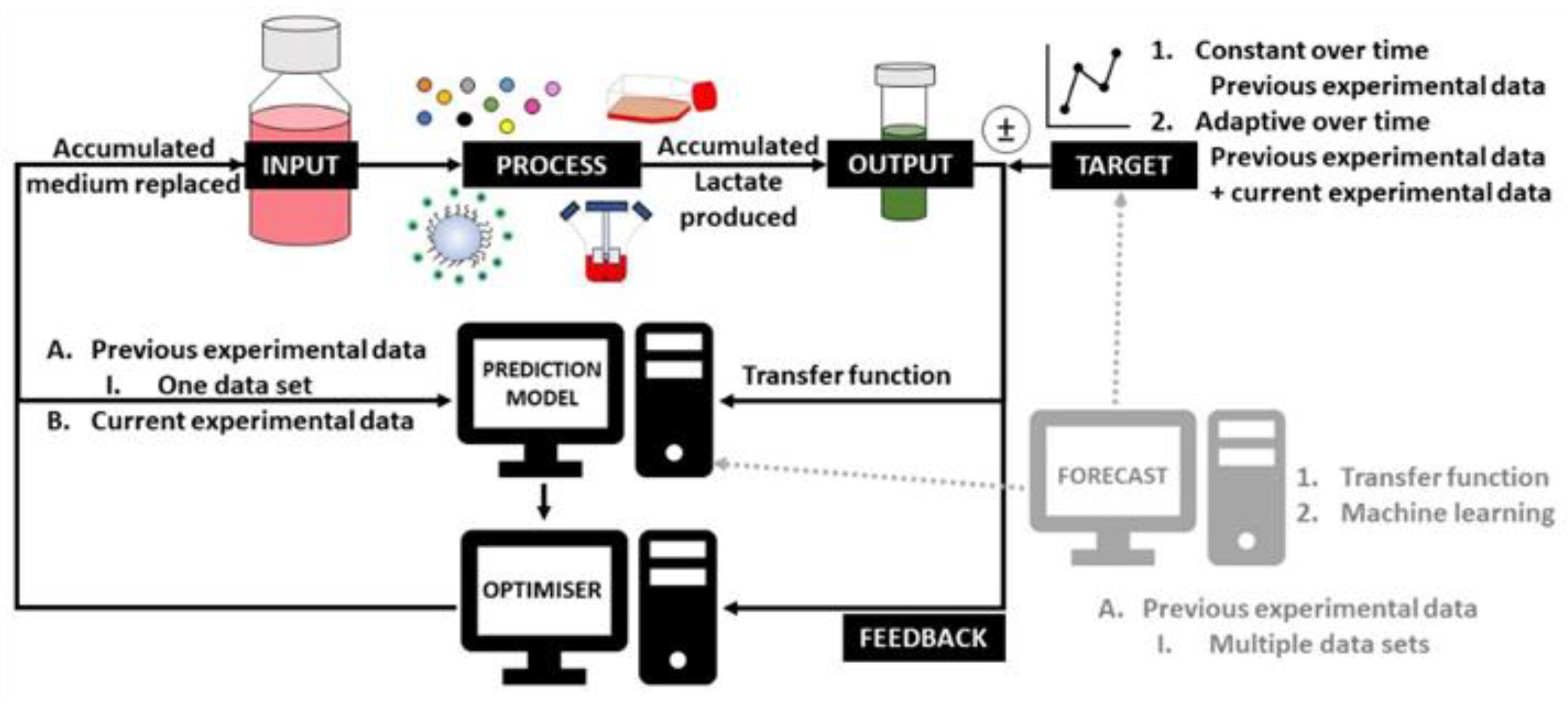
For developing a model predictive controller of a process, having an accurate prediction model and target function is key. Different methods for both estimating the prediction model as well as defining the target function were used in this work and are represented in Figure 1. The prediction model predicts the output of the system based on the previous inputs and outputs of the system. This relation is then used by the controller to calculate the next future input required to minimize the difference between the target and the predicted output. For the prediction model, transfer function models were applied and estimated based on the experimental data. These data were either from the current controller experiment (controller experiment 1) or from a previously performed reference experiment (controller experiment 2). The target function used in the model predictive controller was either predefined (controller experiment 1) or adaptive over time (controller experiment 2). Additional forecasting techniques were performed by applying transfer function models as well as machine learning on multiple previous experimental data simultaneously.

2.3.1. Prediction Model

The first step towards developing a model predictive controller (MPC) was to find a prediction model for the input-output relation that described the dominant processes of the system. In this work, the input used for the prediction model was the accumulated medium replaced and the output was the accumulated lactate produced by the cells.

The controller experiments in this work used a prediction model by applying transfer function models on one experimental dataset as used in previous work [11].

To describe the output as a dynamic response to the input, a dynamic model was estimated through a dynamic auto-regressive with exogenous (DARX) variables model. The model structure of the single-input, single-output discrete time transfer function is given in the following equation [31,32]:

$$y_t = \frac{B\left({\mathrm{z}}^{-1},\mathrm{t}\right)}{A\left({\mathrm{z}}^{-1},\mathrm{t}\right)}{u}_{t - \delta } + \frac{1}{A\left({\mathrm{z}}^{-1},t\right)}{e}_t,$$

(3)

with $y_t$ the output or accumulated lactate (mmol) of the system and $u_{t-\delta }$ the input or accumulated medium replaced (mL). ${\mathrm{z}}^{ - 1}$ is the backward shift operator, $\delta$ is a time delay and $e_t$ is white noise with a zero mean and uncorrelated variance $N\left(0,{\sigma }^2\right)$. The polynomials $A$ and $B$ contain the time-variant model parameters and are described by the following equations:

$$A\left({\mathrm{z}}^{-1},t\right) = 1 + a_{1,t}{\mathrm{z}}^{-1} + a_{2,t}{\mathrm{z}}^{-2} + \dots + a_{n,t}{\mathrm{z}}^{-n_a}$$

(4)

$$B\left({\mathrm{z}}^{-1},t\right) = b_{0,t} + b_{1,t}{\mathrm{z}}^{-1} + b_{2,t}{\mathrm{z}}^{-2} + \dots + b_{m,t}{\mathrm{z}}^{-n_b},$$

(5)

The estimation of the DARX variables was performed using the CAPTAIN toolbox in MATLAB 2021b (The Mathworks, Inc., Natick, MA, USA) [33]. The time-variant parameters describe the changing input-output relation of the system during the different stages of the cell culture period [34].

The best model orders of the polynomials $A$ and $B$ from Equations (4) and (5) together with the time delay were identified using the refined instrumental variable algorithm. The rivid function from the CAPTAIN toolbox selected the best model orders based on the evaluation of the Young identification criteria (YIC) and the coefficient of determination (R²).

The selected model orders were then further used for the estimation of the time-variant parameters. These were estimated using the DARX function from the CAPTAIN toolbox. The normalized root mean square error (NRMSE) was calculated to assess the performance of the prediction model. The NRMSE was calculated using the MATLAB function goodnessOfFit, which compares the values of the measured reference output to the estimated DARX outputs. This calculation is described as follows:

$$\mathrm{NRMSE} = \frac{\Vert y_{ref} - y_{fit}\Vert }{\Vert y_{ref} - mean\left(y_{ref}\right)\Vert },$$

(6)

where $y_{fit}$, the modeled DARX data is compared to $y_{ref}$, the reference data. The NRMSE equal to zero represents a perfect fit.

2.3.2. Optimizer

The model predictive controller used previous input and output measurements to predict future outputs using the prediction model. Next, the predicted outputs were compared with the target function. This error information was than supplied to the optimizer, which considered the constraints and cost function to estimate the required future inputs to minimize the error between the desired output and the real output.

The cost function used by the optimizer is described by

$$J\left(Nc,Np\right) = {{\displaystyle \sum }}_{j = 1}^{Np}\delta \left(j\right){\left[\widehat{y}\left(k + j|k\right) - r\left(k + j\right)\right]}^2 + {{\displaystyle \sum }}_{j = 1}^{Nc}\lambda \left(j\right){\left[∆u\left(k + j - 1\right)\right]}^2,$$

(7)

where the difference between the predicted output ($\widehat{y}$) and the target function (r) is minimized, together with minimizing the change of the control signal ($∆u$) (i.e., the replaced medium volume). $Nc$ is the control horizon, $Np$ is the prediction horizon and $\delta ,\lambda$ are used as weights [31,35].

The MPC was developed using the MPC toolbox in MATLAB, starting with defining the MPC object using the function mpc. The next step was to update this object with the most recently measured output. To integrate the update of the prediction model within this MPC update, the command mpcmoveAdaptive was used.

2.3.3. Target Function

The target function (or reference trajectory) of the controller describes the path to follow for the output values of the system. This path was either predefined following a fixed target function or adaptive over time. Both target functions were based on the measured values of a similar cell expansion, called the reference experiment.

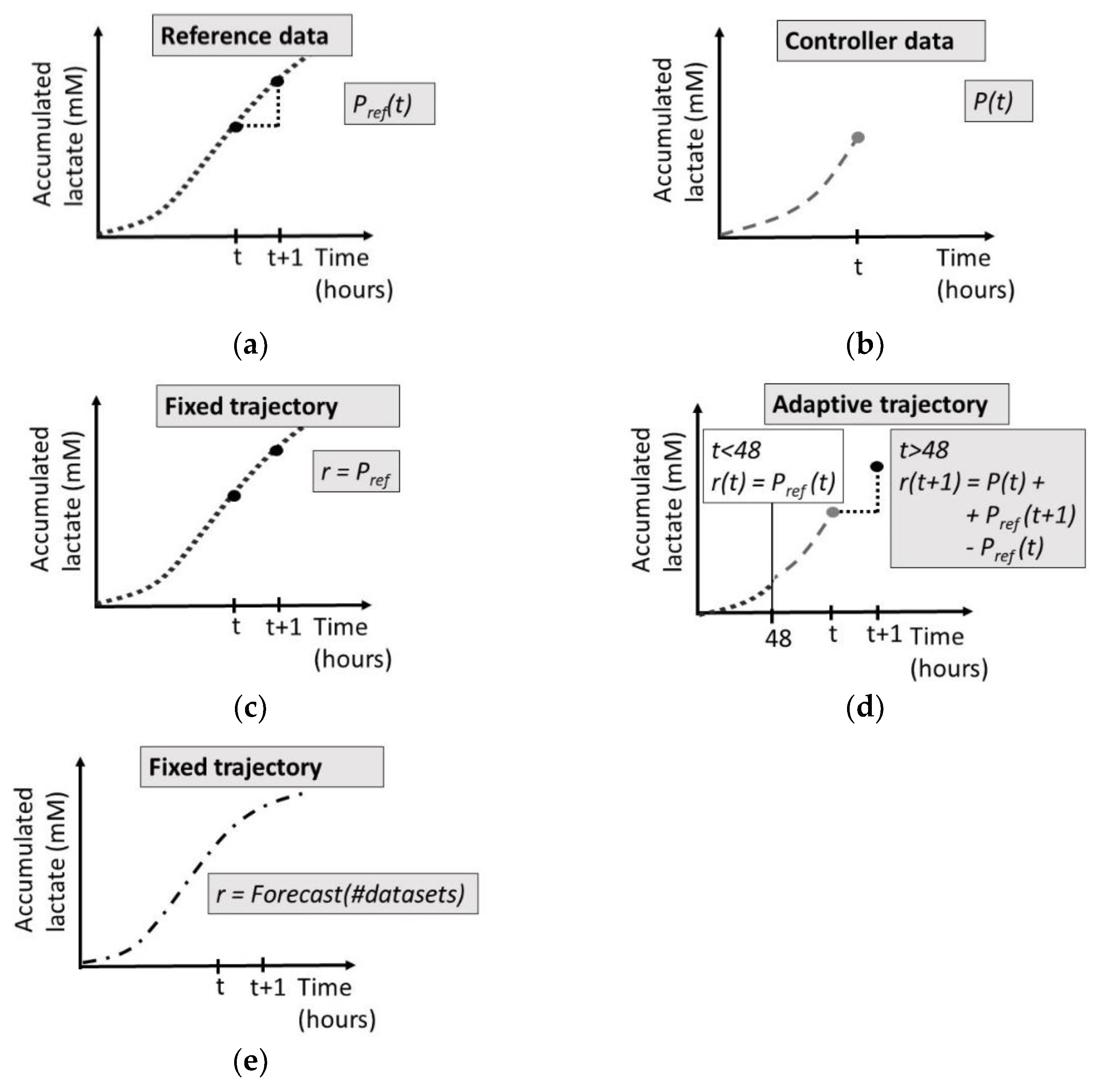
Two types of target functions were addressed in this work, as shown in Figure 2. The first target function was fixed over time (Figure 2c); the defined target function was not changed during the experiment but was defined by one previously performed experiment (Figure 2a) and then further used in controller experiment 1. The second type of target function was adaptive over time (Figure 2d); the defined target function was adapted during the experiment by using ongoing data (Figure 2b) to compensate for over- or under- performing cell batches and then further used in controller experiment 2. As an adaptation of the first type of target function, another target function was also fixed over time (Figure 2e), but was defined by using a forecast based on multiple previously performed experiments. This last method was not applied during experiments in this work, but the forecast method is explained in Section 2.4. Forecasting the Cell Growth Expansion Process, as a possible alternative for defining target functions.

The equations used for the fixed and adaptive target functions of controller experiment 1 and 2 are defined by Equation (8) and by Equation (9), respectively. Equation (9) consists of two parts. The first part, $p\left(t\right)$, makes the trajectory adaptive towards the current controller experiment by updating the target function value at time t to the measured amount of accumulated lactate at time t. The second part, $p_{ref}\left(t + 1\right) - p_{ref}\left(t\right)$, assumes that the increase in accumulated lactate equals the change in accumulated lactate as measured in the reference experiment (Figure 2a).

$$r = p_{ref}.$$

(8)

$$r\left(t + 1\right) = p\left(t\right) + \left[p_{ref}\left(t + 1\right) - p_{ref}\left(t\right)\right],$$

(9)

with $r$ the reference trajectory, $p$ the piecewise linear interpolated data and $p_{ref}$ the piecewise linear interpolated reference data from the initial reference experiment.

2.3.4. Simulation

Before performing the controller experiments, the performance of the controller was evaluated using simulations. This means that the reference data generated from the initial experiment with a fixed predefined medium schedule were used simultaneously as the target function and as past input and output data. Starting after 48 h of initial data collection, the controller used the DARX model of the reference data as a prediction model to estimate the future control input that would generate a future output as close as possible to the target function. The simulation returned a set of control inputs estimated each time for one medium replacement in advance. In addition, the controller predicted the output that would occur after applying the suggested control input.

2.4. Forecasting the Cell Growth Expansion Process

In Section 2.3 (Model Based Control and Optimization) of the work, a prediction model was estimated based on the experimental data gathered during the experiment in which it was used to calculate the control inputs. In contrast to this approach, in this part of the work, a forecast of the cell expansion process is defined based on multiple previously gathered datasets. This forecast could be either used to calculate the control inputs (as described in Section 2.3) or to define the target function of a model predictive controller.

Since the previously described prediction modelling approach (Section 2.3) needs a minimum amount of data to start estimating the model parameters in real-time, ideally, an alternative model should be available to make predictions during the initial period of 48 h, during which the previously described prediction model, using only online data, is gathering enough data to estimate a transfer function after the first 48 h.

As briefly mentioned in Section 2.3.3 (Target Function), a forecast using multiple previously gathered datasets could be useful for defining a robust fixed target function, by including more data than a fixed target function based on data of only one reference experiment.

2.4.1. Transfer Function Approach

To develop a forecast based on several datasets, there are two options when using the DARX databased modelling approach.

The first option fits a different model with a certain set of parameters (a- and b-parameters) for each interpolated dataset of each tissue flask. These are then averaged for the different tissue flasks within the training set. The resulting mean a- and b-parameters are then used for forecasting. To simulate the output of the forecast based on these a and b parameters, Equation (10) was used.

$$y\left(k\right) = \frac{ b_0\left(k\right)}{1 + a_1\left(k\right)z^{-1}}u\left(k - 1\right) + \frac{1}{1 + a_1\left(k\right)z^{-1}}e\left(k\right).$$

(10)

The second option takes the average of the input and output measurements to first design an average dataset. This is only applicable for similar experiments with the same amount of input and output measurements. Due to interpolation, both type of datasets with either every 12 h or every 48 h were combined into one averaged dataset. A forecast for this average dataset is then modelled using again the DARX function in MATLAB.

2.4.2. Machine Learning Approach

This work used a least-squares support vector machine (LS-SVM) regression estimator to forecast the accumulated lactate as a function of the supplied medium. The least squares support vector machines (LS-SVM) toolbox from the department of Electrical Engineering (ESAT) of KU Leuven in Matlab 2021b was used for developing the predictive model [36,37].

The input of the data, the accumulated medium replaced in mL, was pre-processed by normalizing the value to a zero mean. The output of the system was the accumulated lactate in mM.

In order to predict the upcoming output value, we developed an LS-SVM-based time series prediction model. The developed model is a Radial Basis Function (RBF) LS-SVM model. The following equations formulate the working of the RBF LS-SVM [36,37,38,39].

The LS-SVM error loss function is defined as

$$\underset{w,b,e}{\min }\frac{1}{2}{w}^{T}w + \frac{1}{2}\mathsf{\gamma }{{\displaystyle \sum }}_{i = 1}^N{e}_i^2,$$

(11)

while complying to the following constraint

$${\mathrm{y}}_i = w^T\phi \left(x_i\right) + b + e_i, i = 1,\dots ,N,$$

(12)

with γ the regularization parameter, which determines the balance between minimizing the training error and smoothening the estimated function

The Lagrangian is constructed as follows

$$\mathcal{L}\left(w,b,e;\alpha \right) = \frac{1}{2}{w}^{T}w + \frac{1}{2}\mathsf{\gamma }{{\displaystyle \sum }}_{i = 1}^N{e}_i^2 - {{\displaystyle \sum }}_{i = 1}^N{\alpha }_i\left\{w^T\phi \left(x_i\right) + b + e_i - {\mathrm{y}}_i\right\},$$

(13)

with ${\alpha }_i$ the Lagrangian multipliers.

To solve the equation in $\alpha , b$ after eliminating $w, e$, the Kernel function is applied, which in this case is a Radial Basis Function (RBF) kernel. This RBF kernel function replaces the dot product as follows:

$$\phi {\left(x\right)}^T\phi \left(x_i\right) = K\left(x,x_i\right)$$

(14)

$$K\left(x,x_i\right) = exp\left(-\frac{{\Vert x - x_i\Vert }^2}{2{\sigma }^2}\right)$$

(15)

with ${\sigma }^2$ the kernel function parameter, which results in the RBF LS-SVM model for function estimation as described by the following equation.

$$y(x) = {{\displaystyle \sum }}_{i = 1}^N{\alpha }_{i}K(x,x_i) + b$$

(16)

The model’s hyperparameters (γ and ${\sigma }^2$) of the RBF LS-SVM are tuned using a 10-fold cross validation approach.

2.4.3. Evaluation Forecast Using Multiple Datasets

The developed predictive model is evaluated using the leave-one-out method by iteratively training the model with all data points except one to be used to test the model. The error performance of the model is evaluated using the NRMSE error metric.

3. Results

3.1. Experimental Data

During 2D cell growth, cells progressively cover the entire available culture surface, Figure 3 shows typical low, mid, and high confluency over time. For quantitative analysis of cell growth, cell counts were also performed; the results of the cell expansions of the reference experiment as well as both controller experiments are summarized in

Table 4. Cell expansion results from the reference experiment. Number of cells counted, total amount of accumulated lactate produced (mM), total amount of medium supplied (mL) and the overall medium efficiency (cells/mL).

	TF1	TF2	TF3	TF4	TF5	TF6	TF7	TF8
Cells counted (1.0 × 106)	3.13	2.79	3.26	2.97	1.74	1.29	1.27	0.65
Accumulated lactate (mM)	15.81	15.48	13.86	14.70	7.21	6.74	6.79	6.91
Accumulated medium (mL)	95.00	95.00	68.75	68.75	95.00	95.00	68.75	68.75
Medium efficiency (1.0 × 104 cells/mL)	3.29	2.93	4.73	4.32	1.83	1.36	1.85	0.95

,

Table 5. Cell expansion results from the first controller experiment. Number of cells counted, total amount of accumulated lactate produced (mM), total amount of medium supplied (mL) and the overall medium efficiency (cells/mL).

	TF1	TF2	TF3	TF4	TF5	TF6	TF7	TF8
Cells counted (1.0 × 106)	1.15	1.20	1.03	0.93	1.21	1.23	1.04	0.92
Accumulated lactate (mM)	8.29	8.27	8.45	8.55	10.40	9.83	9.22	9.73
Accumulated medium (mL)	151.25	96.25	96.88	64.38	79.07	56.45	73.01	53.20
Medium efficiency (1.0 × 104 cells/mL)	0.76	1.24	1.06	1.44	1.53	2.18	1.42	1.72

and

Table 6. Cell expansion results from the second controller experiment. Number of cells counted, total amount of accumulated lactate produced (mM), total amount of medium supplied (mL) and the overall medium efficiency (cells/mL).

	TF1	TF2	TF3	TF4	TF5	TF6	TF7	TF8
Cells counted (1.0 × 106)	2.72	2.49	2.34	2.28	2.53	2.45	2.54	2.44
Accumulated lactate (mM)	13.80	13.15	13.29	12.98	13.47	13.07	12.78	13.34
Accumulated medium (mL)	93.79	95.71	95.53	95.00	84.71	86.83	87.73	95.00
Medium efficiency (1.0 × 104 cells/mL)	2.90	2.60	2.45	2.39	2.98	2.82	2.89	2.59

.

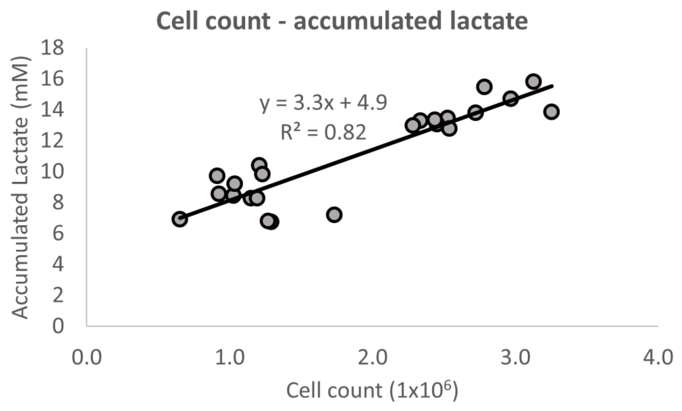
To assess the correlation between cell counts and accumulated lactate, all data points from the three different experiments were plotted in Figure 4. A significantly different value from zero trendline was fitted through the data with an R² equal to 0.82.

3.2. Prediction Model

A prediction model applying transfer function models on one dataset was used in the controller experiments. The collected data from the reference experiments were used to identify which model order would be best to describe the process. The use of the rivid function in Matlab identified the [1 1 1] model order as the best suited model based on the YIC and R² criteria (Equation (10)).

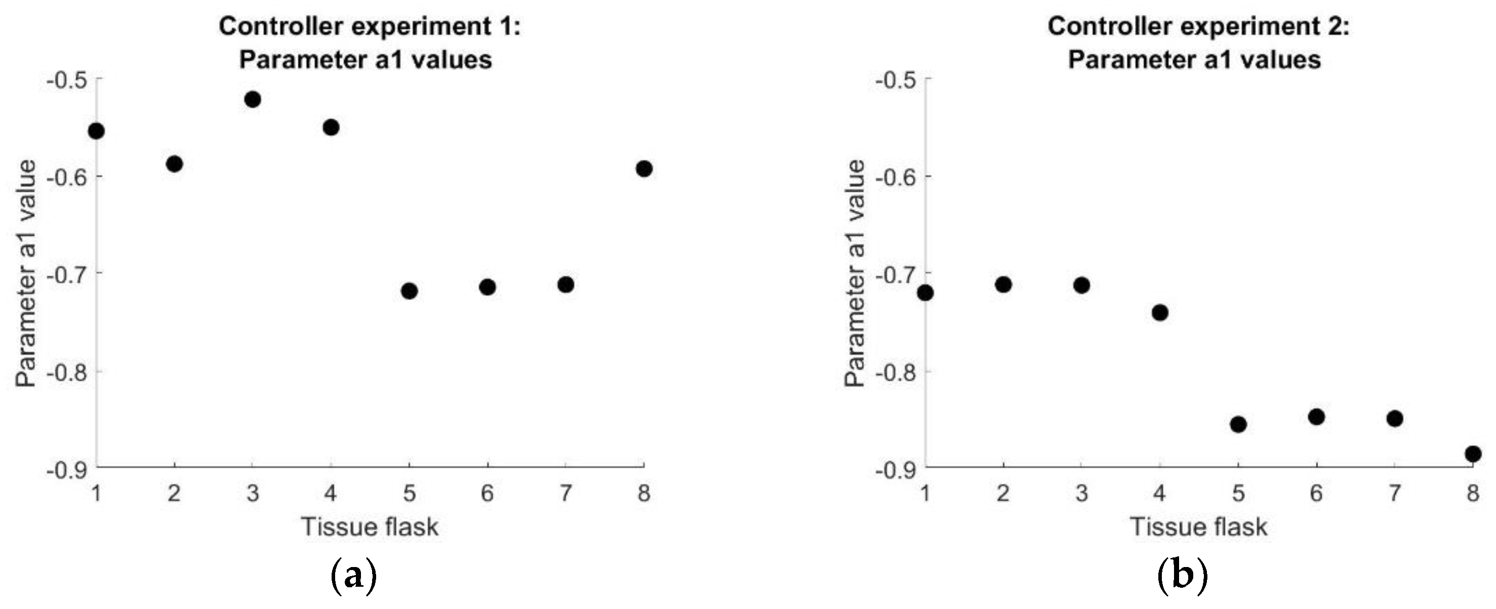
The DARX [1 1 1] model resulted in an a₁ parameter with minimal variation over time. Therefore, it was decided to keep the a₁ parameter fixed in time while allowing the b₀ to be time-variant. By fixing one of the two parameters, the computational complexity is reduced and the mechanistic understanding is simplified, since only one parameter (b₀) explains the variation of the model over time. The DARX [1 1 1] was evaluated as a prediction model based on the normalized root mean square error (NRMSE), which was calculated using the goodnessOfFit function in MATLAB. The NRMSE compares the simulated output predicted by the DARX function with the experimental data and is represented in

Table 7. NRMSE, model evaluation of the DARX [1 1 1] model for the data of all eight tissue flasks for all three experiments. A NRMSE equal to zero represents a perfect fit of the DARX model when compared to the experimental data.

	NRMSE
	Reference Exp	Controller Exp 1	Controller Exp 2
TF1	0.0115	0.0148	0.0088
TF2	0.0016	0.0048	0.0122
TF3	0.0074	0.0140	0.0010
TF4	0.0077	0.0166	0.0021
TF5	0.0155	0.0017	0.0130
TF6	0.0021	0.0033	0.0038
TF7	0.0027	0.0010	0.0142
TF8	0.0093	0.0010	0.0023

.

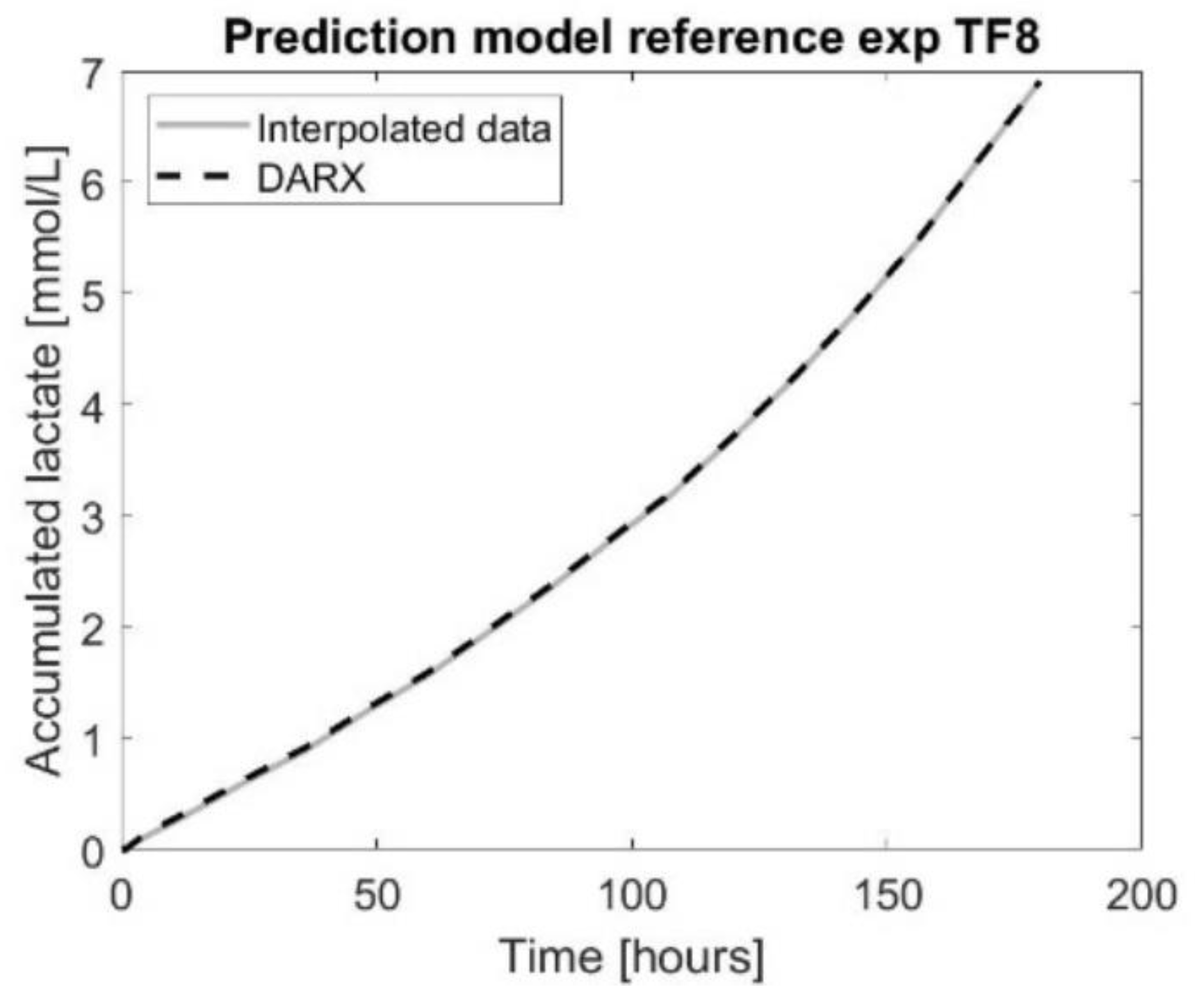
The visualisation of the DARX model compared to the interpolated experimental data is presented in Figure 5.

3.3. Controller Experiments

3.3.1. Controller Experiment One

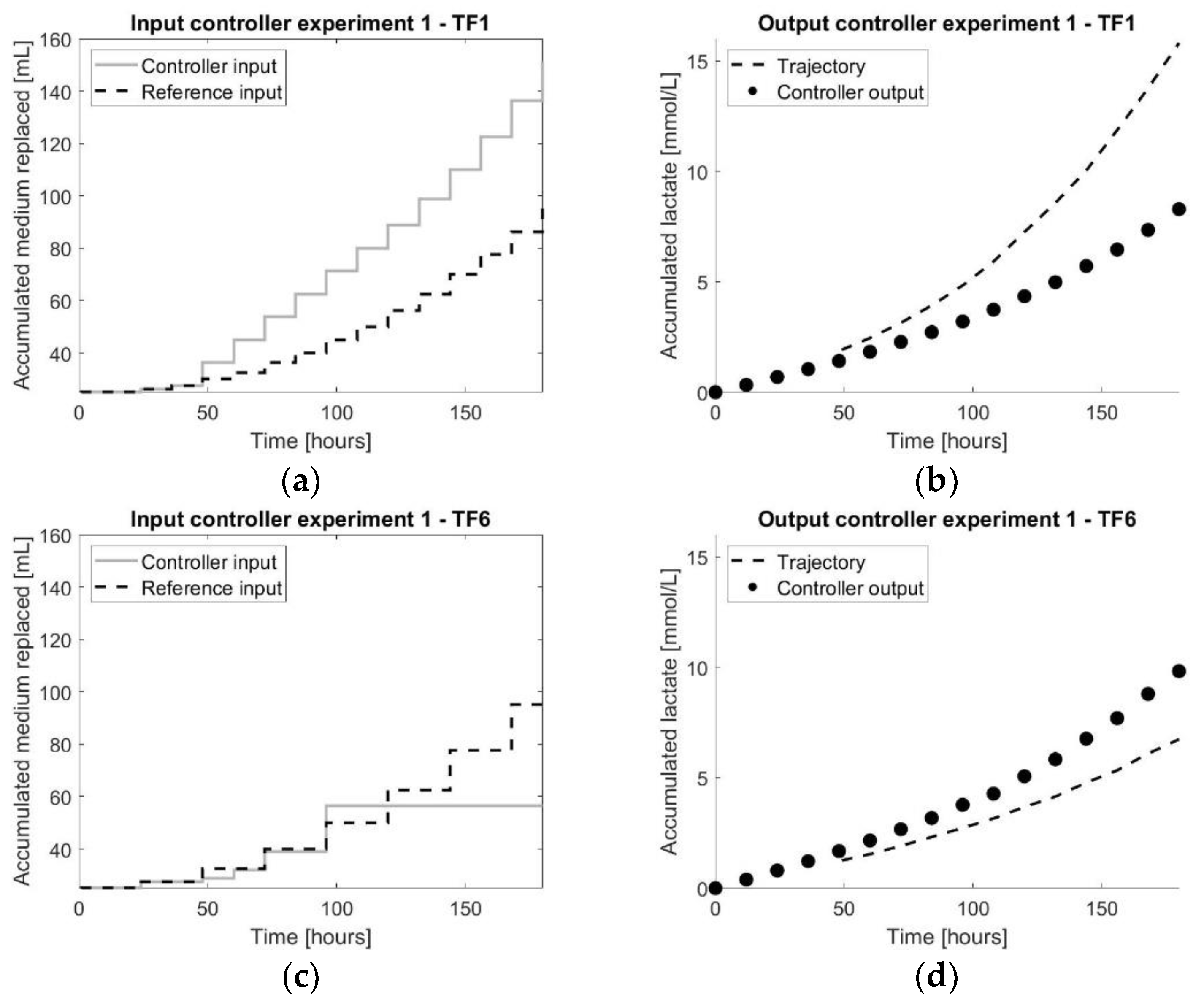
The results of the controller experiments performed using a fixed target function in time based on the accumulated lactate values of the reference experiment are shown in Figure 6 and

Table 8. NRMSE values comparing the accumulated lactate output values of the controller experiment one with the trajectory values using the goodnessOfFit function in MATLAB. The NRMSE closer to zero represents the better fit.

	TF1	TF2	TF3	TF4	TF5	TF6	TF7	TF8
NRMSE	0.9107	0.9091	0.8739	0.8485	0.9125	1.0486	0.7550	0.9637

.

3.3.2. Controller Experiment Two

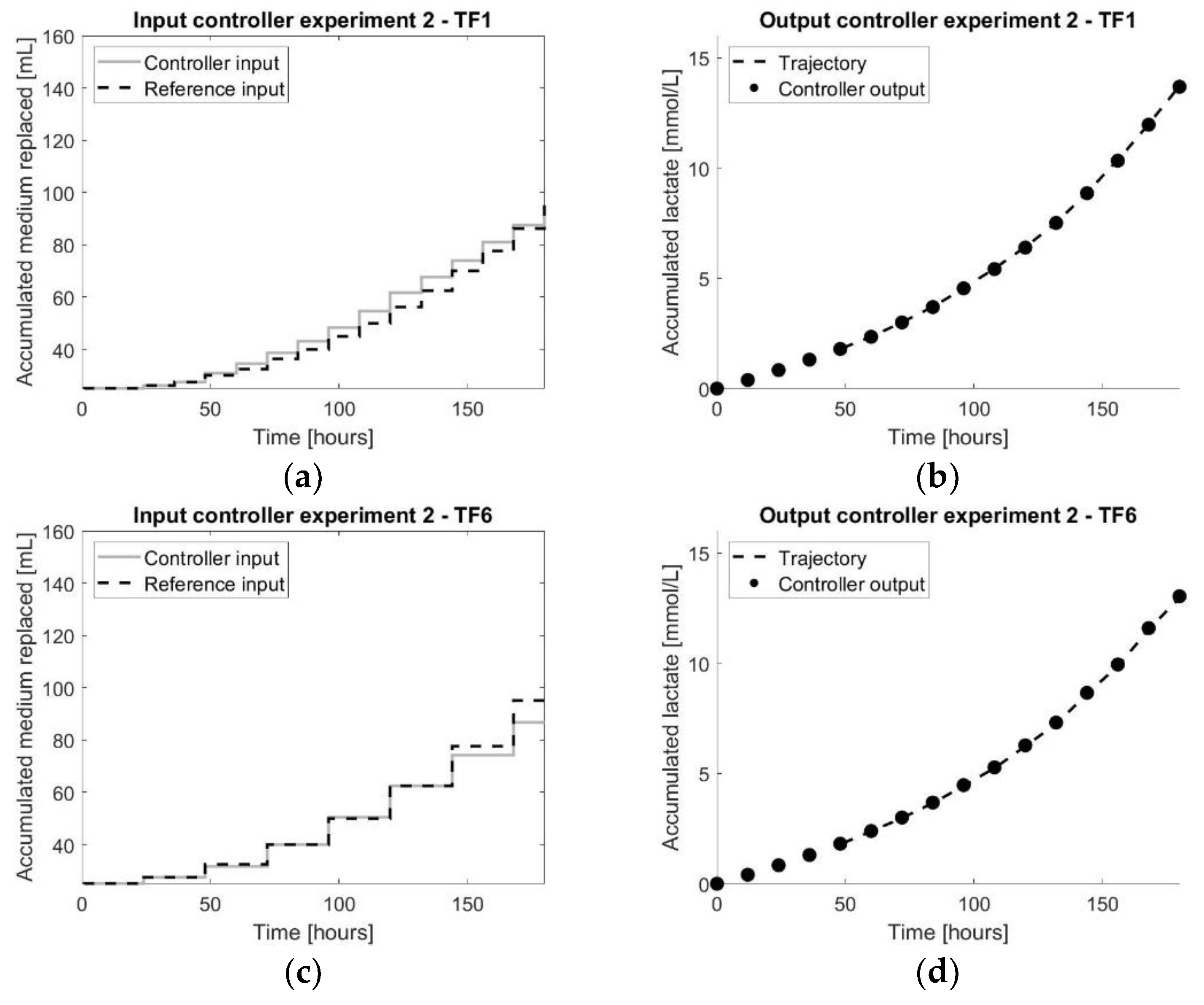
The results of the controller experiments using and adaptive target function in time are shown in Figure 7 and

Table 9. NRMSE values comparing the accumulated lactate output values of the controller experiment two with the trajectory values using the goodnessOfFit function in MATLAB. The NRMSE closer to zero represents the better fit.

	TF1	TF2	TF3	TF4	TF5	TF6	TF7	TF8
NRMSE	0.0054	0.0071	0.0068	0.0073	0.0149	0.0145	0.0143	0.0147

. The MPC from this second controller experiment used an adaptive target function.

3.4. Forecasting the Cell Expansion Process Using Multiple Datasets

The results of forecasting the cell expansion process using multiple datasets for the transfer function and machine learning models applied to the data of the eight different tissue flasks of the second controller experiment are represented below.

3.4.1. Transfer Function

Averaging Parameter Values

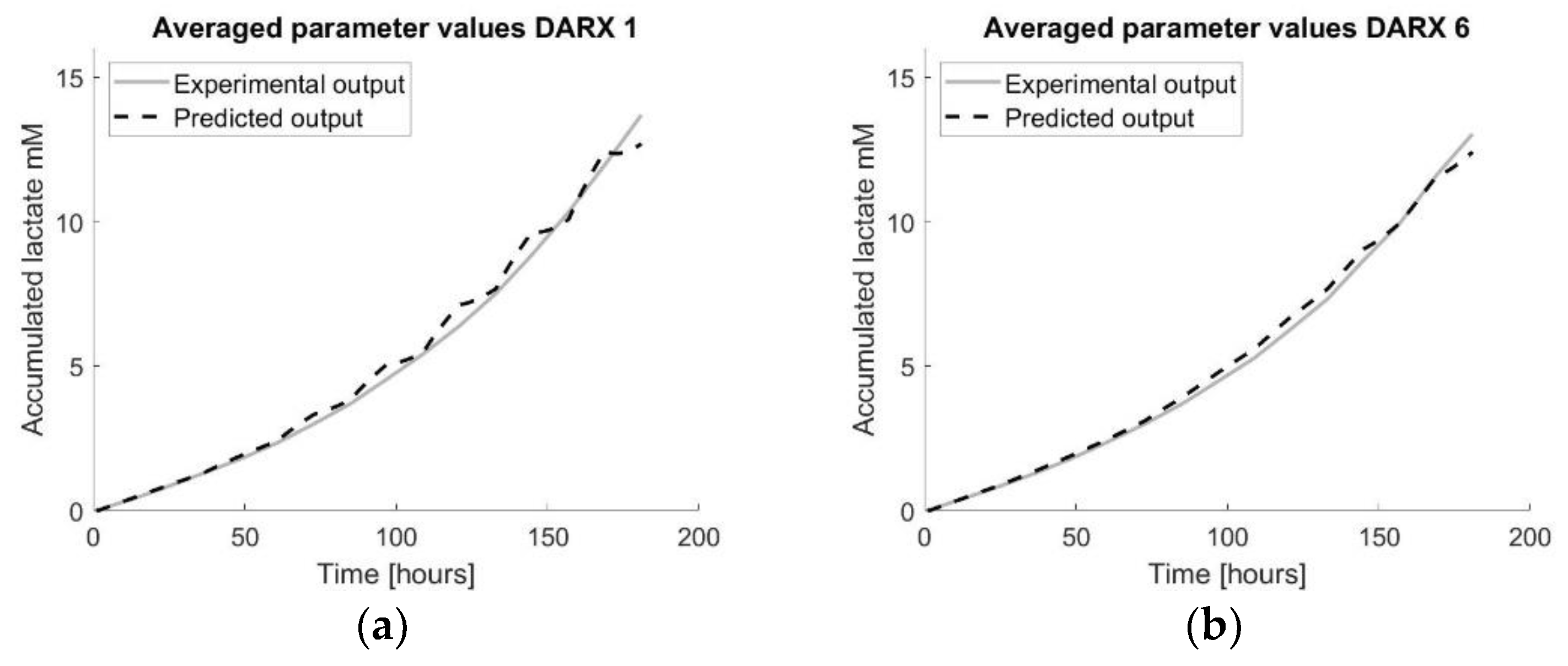
The first method to apply transfer function models on different datasets was to apply transfer functions onto all different datasets and averaging the different a- and b-parameters of the DARX model into one transfer function. These results are shown in Figure 8 and

Table 10. NRMSE comparing the accumulated lactate output values of the forecast model using multiple datasets by applying DARX transfer function models on the different datasets and averaging the parameters using the goodnessOfFit function in MATLAB. The NRMSE closer to zero represents the better fit. The number of the tissue flasks referrers to the tissue flask used as the test data set.

	TF1	TF2	TF3	TF4	TF5	TF6	TF7	TF8
NRMSE	0.0846	0.1441	0.1319	0.0647	0.0752	0.0647	0.0927	0.0023

.

Averaging Data

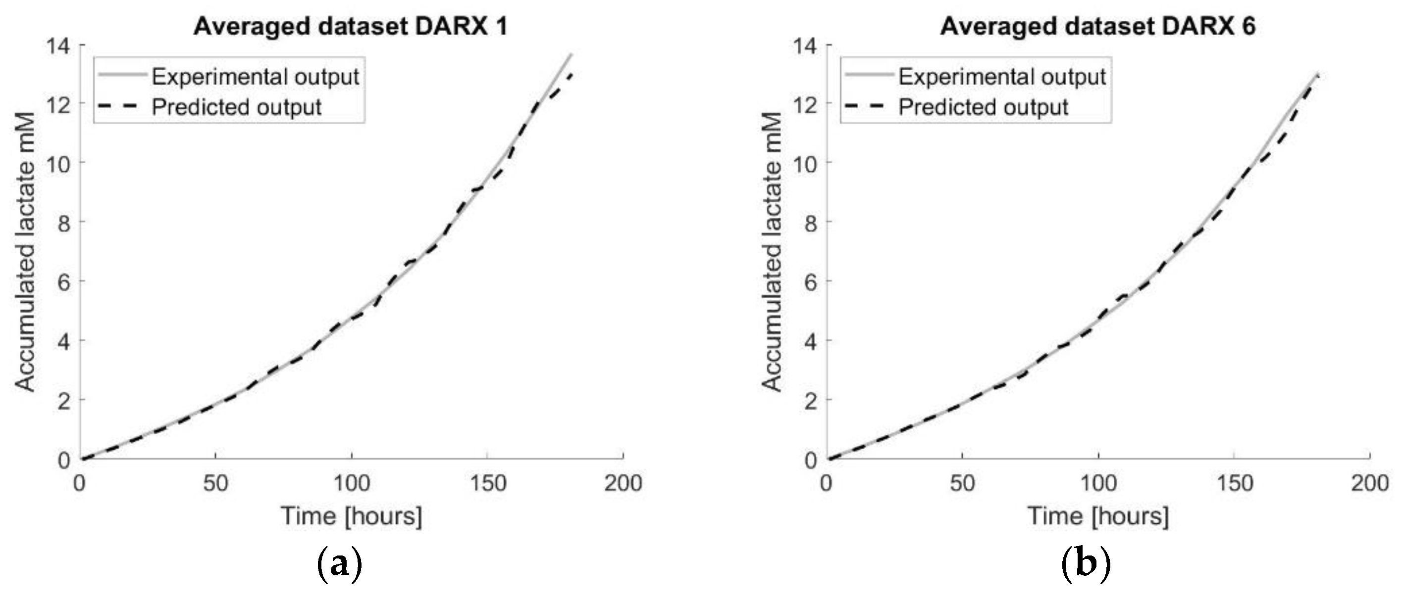
This second method to apply transfer function models on different datasets was to average all the datasets together into one dataset before applying the transfer function DARX. These results are shown in Figure 9 and

Table 11. NRMSE comparing the accumulated lactate output values of the forecast model using multiple datasets by applying DARX transfer function models on the averaged dataset using the goodnessOfFit function in MATLAB. The NRMSE closer to zero represents the better fit.

	TF1	TF2	TF3	TF4	TF5	TF6	TF7	TF8
NRMSE	0.0439	0.0932	0.0876	0.0443	0.1037	0.0431	0.0682	0.0849

.

3.4.2. Machine Learning

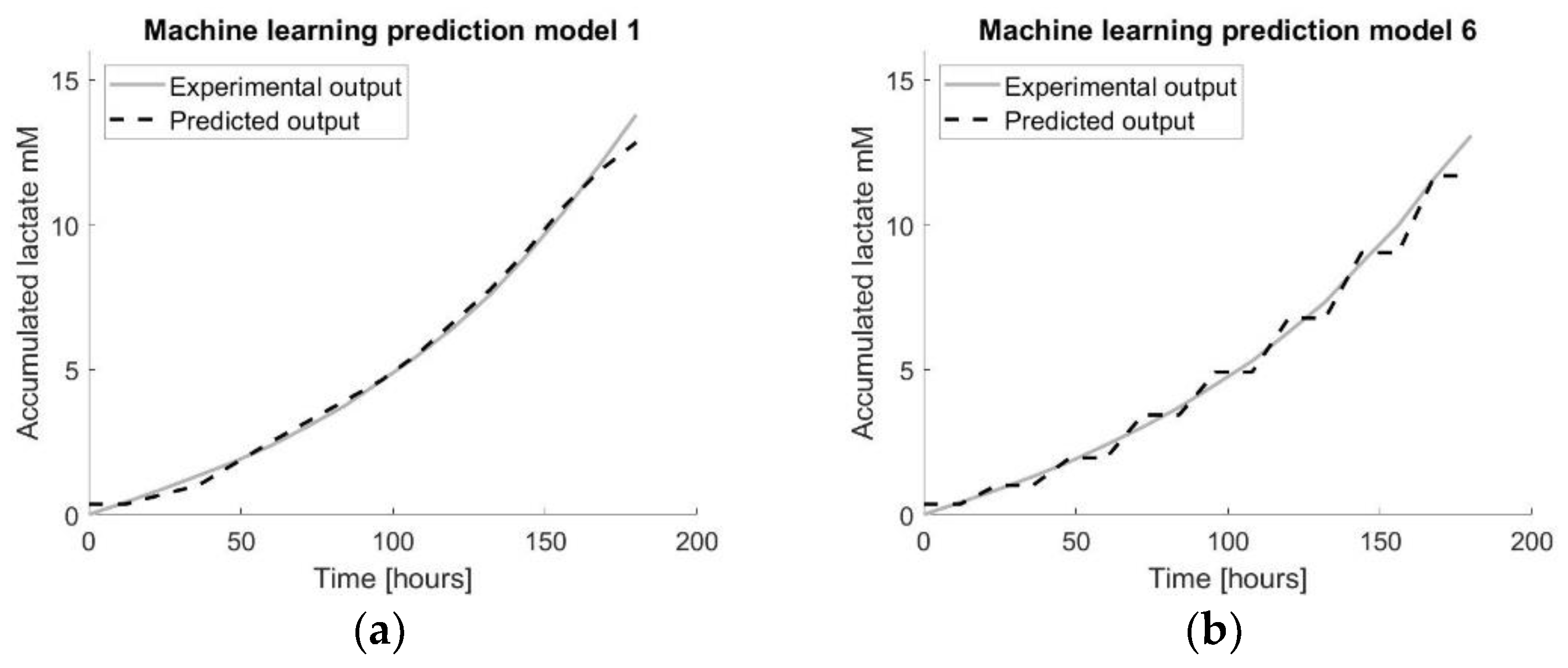
The results of applying machine learning on multiple datasets are shown in Figure 10 and

Table 12. NRMSE comparing the accumulated lactate output values of the forecast model using multiple datasets by applying machine learning using the goodnessOfFit function in MATLAB. The NRMSE closer to zero represents the better fit. The number of the tissue flasks referrers to the tissue flask used as the test data set.

	TF1	TF2	TF3	TF4	TF5	TF6	TF7	TF8
NRMSE	0.0917	0.1292	0.1094	0.0644	0.1944	0.1300	0.1145	0.1740

.

3.5. Mechanistic Understanding of the Transfer Function Model

To understand the dynamics of the cell expansion system, the changing relation of the output compared to the input was investigated. Since the best DARX model resulted in a fixed $a_1$ parameter over time and a time-variant $b_0$ parameter, the output to input relation can be approximated by b₀ when using the steady state gain response of Equation (17):

$$SSG = \frac{ b_0\left(k\right)}{1 + a_1}.$$

(17)

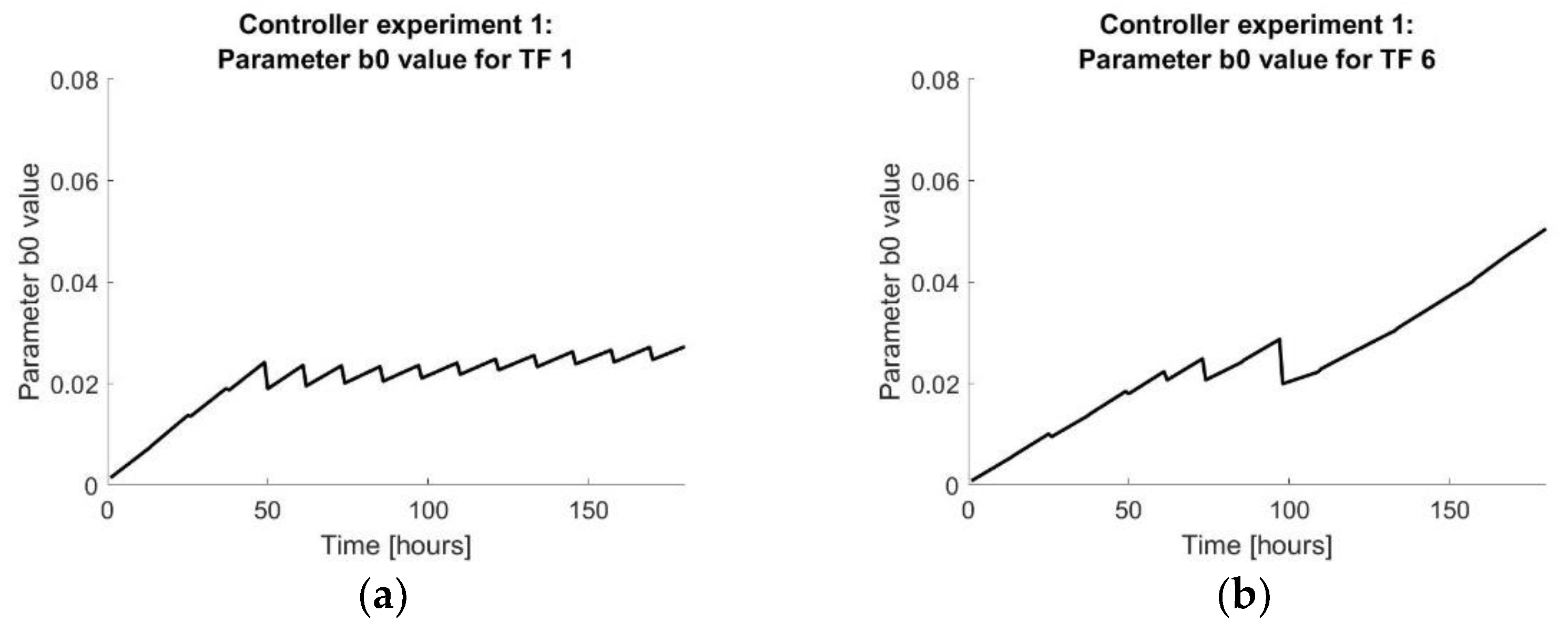
The steady state gain can be interpreted as the change of output (accumulated lactate produced) per unit change of input (amount of medium spent) and can be approximated by the $b_0$ value. To understand the effect of a change in the $b_0$ value, different cases during the controller experiments were observed. A different first order DARX transfer function was applied on each of the eight tissue flasks of both controller experiments. The fixed $a_1$ parameters of the resulting DARX model for all tissue flasks of both controller experiments are shown in Figure 11. The time-variant $b_0$ parameter of TF1 and TF6 of both controller experiments are shown in Figure 12.

The first case occurred during controller experiment 1 for tissue flasks 1 until 4. In this case, the cells were not producing as much lactate as the reference and they were pushed to grow faster by supplying more medium. However, the target function was not realistic, resulting in overfeeding the cells compared to the reference. At each medium replacement, the $b_0$ value drops and afterwards rises again, resulting in a more or less constant $b_0$ value. This then relates back to a constant ratio of accumulated lactate over accumulated medium supplied.

The second case occurred during controller experiment 1 for tissue flasks 5 until 8. Here, the cells were producing more lactate than the target function, resulting in underfeeding the cells after four days, compared to the reference. Therefore, the amount of lactate produced compared to the amount of medium supplied increases, which is also visible in the increasing $b_0$ value. This would mean that the amount of medium supplied for the same amount of lactate produced is lowering throughout the cell expansion process.

There is a balance between supplying the right amount of medium for the cells to grow efficiently. The cells should not be underfed or overfed as this unnecessarily increases the costs of the process. The ideal ratio of lactate versus medium and then the $b_0$ value will depend on whether the total number of cells at the end of the expansion or the total cost of the expansion is more important. It would be interesting to obtain additional data regarding clear overfeeding and underfeeding of the cells to observe what the $b_0$ value and final cell counts would be.

4. Discussion

Cell culture processes involving living systems are still far from being perfectly monitored and controlled as compared to chemical production processes [40,41,42,43]. This is because biosystems are complex, individually different, time-varying and dynamic [44]. The cell characteristic depends on many factors including the passage number, donor age, seeding density and medium replacement strategy, all of which affect the presence of nutrients and metabolic by-products [14,45,46]. In case a chemical process starts from a raw material that has a certain deviation from the standard raw material, the process can be adapted taking this initial deviation into account. However, whether a certain cell batch will grow faster or slower than the ‘standard’ batch cannot be predicted or measured like a physical characteristic of a raw material in a chemical process. Therefore, it is an advantage to apply an adaptive control strategy that will learn the characteristics of the considered cell batch and adapt to it as quickly as possible.

This work developed a data-based model predictive controller, in order to steer the cell expansion process towards an adaptive target function. The medium supplied to the system was considered as the control input, while the measured lactate production was used as the output of the system. The advantage of using accumulated lactate produced by the cells as output is that it can be measured during the process non-invasively as an indicator for cell growth. The correlation between cell growth and accumulated lactate was demonstrated and visualized in Figure 4, where the total amount of lactate produced by the cells follows the same trend as the number of cells counted at the end of the expansion process over the different tissue flasks. The R² of the linear trendline between the two variables is 82% and is significantly different from zero. Other possible output variables selected in literature have been glucose [19,20] or dissolved oxygen [47]. The accumulated medium was selected as the input of the system because it has a direct impact on the cell growth by removing toxic waste products (lactate) and introducing energy sources (glucose) and growth factors [48]. In addition, as the medium replacement rate has a direct impact on the cost of the cell production process, optimizing this input will directly influence the operating cost of the cell expansion.

Controller experiment 1 tried to mimic the exact amount of lactate produced by the cells in the reference experiment. For tissue flasks 1 until 4, this meant giving the cells more medium than the reference, and for tissue flask 5 until 8, this meant less medium. However, due to cell donor variability, the controller was not capable of reproducing the same number of cells for tissue flasks 1 until 4. Although the controller provided more medium than the reference experiment, there were less cells in the end. The controller tried to cope with the slower growing cells or the lower number of cells. Since the cells produced a lower amount of lactate than the reference experiment, the controller saw this as a reason to give more medium than used during the reference experiment. However, the higher supply of medium did not seem to cover the lack of growth, and therefore, the system was unable to achieve the same number of cells at the end. For tissue flasks 5 until 8, the full capacity of the cells was not used. By only using information of the initial reference experiment to define the trajectory, fast growing cells that require more medium were starved to slow their growth down towards the reference trajectory. The conclusion here is that it is suboptimal to use a general reference trajectory based on predefined lactate values for a new experiment since each batch of cells is very different.

Controller experiment 2 used real-time process information to form an adaptive target trajectory. In addition to the values of the accumulated lactate concentrations of the reference experiment, the online information of the considered cell expansion process in the optimization of the process was also included in the adaptive target trajectory. In this way, the full potential of the cells was used, meaning that the cells were fed according to their needs, without under or overfeeding them as was the case in the first controller experiment. To have a better understanding of how the controller works for different groups, it would be interesting to perform future experiments where the controller is applied to more than one cell line or to even use another output measurement instead of accumulated lactate.

As a case study, we used results from the controller experiment 2 in order to simulate how much medium could be saved on a whole cell expansion process by following the controller’s suggestions regarding medium replacements, without decreasing the number of obtained cells. Therefore, the amount of medium saved from the triplicate flasks number 5, 6, and 7 was compared to their control flask 8. This resulted in an average of 86.42 mL medium used compared to 95 mL, which is equal to 9% medium saved. The number of cells was not decreased due to this medium reduction; there was even a slight average increase of 6.66 × 10⁶ cells. When simulating this for a whole cell expansion process going from 0.25 × 10⁶ cells from biopsy to a total of 1 × 10⁸ cells, additional information from the controller experiments was used. The seeding density of 2500 cells/cm², together with the average harvesting density of 14,285 cells/cm², would result in a sequence of expansions of tissue flask 175 going from one TF175 to 5, to 28 and finally to 40. When adding up the 8.58 mL of medium saved for each expansion, this would result in a total of 634.92 mL medium saved.

The collected data from controller experiment 2 were also used to forecast the cell expansion process by using the combined data of several experimental runs together. These forecasting techniques could be used in future work either in the prediction model or as a target function. The first forecast method used transfer functions as previously used in the prediction models of the controller experiments. Both methods of either averaging the model parameters or averaging the datapoints for the DARX modelling approach resulted in similar accuracies of the forecasts. The second forecast method used machine learning, more specifically LS-SVM, which uses the forecasting model as a machine learning algorithm.

A next step could be to use other machine learning algorithms, such as k-nearest neighbours LS-SVM [49] and compare both. Since the power of machine learning was not fully accessed in this work due to the small size of the dataset, a valuable future approach would be to gather a large dataset with many possible input and output variables and release the power of machine learning on such data. Including information on donor characteristics as well as other relevant process variables could benefit the optimization of the cell expansion process. In this way, we expect the machine learning-based approach to outperform the transfer function-based approach.

Another interesting future work would be to start with a medium supply scheme based on predefined knowledge of the cell batch using machine learning [14] or mechanistic models [50] (e.g., to predict the cell growth) followed by the control strategy using DARX transfer functions to adapt the medium supply based on the accumulated lactate measured. Using knowledge and/or data from previous experiments through mechanistic and machine learning models has the advantage that a more personalized feeding strategy can be applied at the start of the cell proliferation process. Once enough data are gathered during an initial period, the applied transfer function modelling approach using real-time data will take into account the specific individual and time-varying characteristics of the considered cell growth process and the medium supply scheme can be adapted accordingly.

Mechanistic modelling and transfer function modelling approaches could also be combined. One way to do so is by using the mechanistic model for generating or simulating process data on which a transfer function model is then applied, resulting in a compact process model focusing only on the dominant processes influencing the cell growth. Via statistical emulation approaches, the parameters of such higher order mechanistic models can be mapped onto the dominant modes of a reduced-order transfer function, allowing to describe the process with a compact transfer function model with biologically interpretable parameters [51]. Another integration of a mechanistic model into the control strategy is to use it for estimating the target trajectory of the cell growth process. This mechanistic model could be similar as the one described by Guyot, but adapted and calibrated for a spinner flask experiment [50].

5. Conclusions

This work developed a data-based model predictive controller for steering cell growth processes towards an adaptive target function. Applying an adaptive target function has proven to be a big advantage compared to a fixed predefined target function. The adaptive nature of the target function allows taking into account the different characteristics of each cell batch, resulting in a personalized and optimized feeding strategy for each cell batch. In addition, a method to combine the data from multiple experimental runs into one model to forecast the cell expansion process was designed by applying either transfer function models or machine learning.

References

1. Detela, G.; Lodge, A. EU Regulatory Pathways for ATMPs: Standard, Accelerated and Adaptive Pathways to Marketing Authorisation. Mol. Ther. Methods Clin. Dev. 2019, 13, 205–232. [Google Scholar] [CrossRef] [PubMed] [Green Version]
2. Emerson, J.; Glassey, J. Bioprocess monitoring and control: Challenges in cell and gene therapy. Curr. Opin. Chem. Eng. 2021, 34, 100722. [Google Scholar] [CrossRef]
3. Jung, S.; Panchalingam, K.M.; Wuerth, R.D.; Rosenberg, L.; Behie, L.A. Large-scale production of human mesenchymal stem cells for clinical applications. Biotechnol. Appl. Biochem. 2012, 59, 106–120. [Google Scholar] [CrossRef]
4. Simaria, A.S.; Hassan, S.; Varadaraju, H.; Rowley, J.; Warren, K.; Vanek, P.; Farid, S.S. Allogeneic cell therapy bioprocess economics and optimization: Single-use cell expansion technologies. Biotechnol. Bioeng. 2014, 111, 69–83. [Google Scholar] [CrossRef] [PubMed] [Green Version]
5. Lipsitz, Y.Y.; Timmins, N.E.; Zandstra, P.W. Quality cell therapy manufacturing by design. Nat. Biotechnol. 2016, 34, 393–400. [Google Scholar] [CrossRef]
6. Schop, D.; Janssen, F.W.; Van Rijn, L.D.S.; Fernandes, H.; Bloem, R.M.; De Bruijn, J.D.; Van Dijkhuizen-Radersma, R. Growth, Metabolism, and Growth Inhibitors of Mesenchymal Stem Cells. Tissue Eng. Part A 2009, 15, 1877–1886. [Google Scholar] [CrossRef]
7. Patel, S.D.; Papoutsakis, E.T.; Winter, J.N.; Miller, W.M. The Lactate Issue Revisited: Novel Feeding Protocols to Examine Inhibition of Cell Proliferation and Glucose Metabolism in Hematopoietic Cell Cultures. Biotechnol. Prog. 2000, 16, 885–892. [Google Scholar] [CrossRef] [PubMed]
8. Folmes, C.D.L.; Dzeja, P.P.; Nelson, T.J.; Terzic, A. Metabolic Plasticity in Stem Cell Homeostasis and Differentiation. Cell Stem Cell 2012, 11, 596–606. [Google Scholar] [CrossRef] [Green Version]
9. Sobacchi, C.; Palagano, E.; Villa, A.; Menale, C. Soluble Factors on Stage to Direct Mesenchymal Stem Cells Fate. Front. Bioeng. Biotechnol. 2017, 5, 32. [Google Scholar] [CrossRef] [PubMed]
10. Van Beylen, K. Decision-Support Tool for Optimal Stem Cell Expansion in Bioreactors. Master’s Thesis, Katholieke Universiteit Leuven, Leuven, Belgium, May 2016. [Google Scholar]
11. Van Beylen, K.; Youssef, A.; Fernández, A.P.; Lambrechts, T.; Papantoniou, I.; Aerts, J.-M. Lactate-Based Model Predictive Control Strategy of Cell Growth for Cell Therapy Applications. Bioengineering 2020, 7, 78. [Google Scholar] [CrossRef]
12. Rafiq, Q.A.; Coopman, K.; Nienow, A.W.; Hewitt, C.J. A quantitative approach for understanding small-scale human mesenchymal stem cell culture—Implications for large-scale bioprocess development. Biotechnol. J. 2013, 8, 459–471. [Google Scholar] [CrossRef] [PubMed] [Green Version]
13. Eibes, G.; dos Santos, F.; Andrade, P.Z.; Boura, J.S.; Abecasis, M.M.; da Silva, C.L.; Cabral, J.M. Maximizing the ex vivo expansion of human mesenchymal stem cells using a microcarrier-based stirred culture system. J. Biotechnol. 2010, 146, 194–197. [Google Scholar] [CrossRef] [PubMed]
14. Mehrian, M.; Lambrechts, T.; Marechal, M.; Luyten, F.P.; Papantoniou, I.; Geris, L. Predicting in vitro human mesenchymal stromal cell expansion based on individual donor characteristics using machine learning. Cytotherapy 2020, 22, 82–90. [Google Scholar] [CrossRef] [PubMed]
15. Martínez-Monge, I.; Martínez, C.; Decker, M.; Udugama, I.A.; de Mas, I.M.; Gernaey, K.V.; Nielsen, L.K. Soft-sensors application for automated feeding control in high-throughput mammalian cell cultures. Biotechnol. Bioeng. 2022, 119, 1077–1090. [Google Scholar] [CrossRef] [PubMed]
16. Brunner, V.; Siegl, M.; Geier, D.; Becker, T. Challenges in the Development of Soft Sensors for Bioprocesses: A Critical Review. Front. Bioeng. Biotechnol. 2021, 9, 730. [Google Scholar] [CrossRef] [PubMed]
17. U.S. Department of Health and Human Services Food and Drug Administration. Guidance for Industry PAT—A Framework for Innovative Pharmaceutical Development, Manufacturing, and Quality Assurance; FDA: Silver Spring, MD, USA, 2004. [Google Scholar]
18. Guadix, J.A.; López-Beas, J.; Clares, B.; Soriano-Ruiz, J.L.; Zugaza, J.L.; Gálvez-Martín, P. Principal Criteria for Evaluating the Quality, Safety and Efficacy of hMSC-Based Products in Clinical Practice: Current Approaches and Challenges. Pharmaceutics 2019, 11, 552. [Google Scholar] [CrossRef] [PubMed] [Green Version]
19. Goldrick, S.; Lee, K.; Spencer, C.; Holmes, W.; Kuiper, M.; Turner, R.; Farid, S.S. On-Line Control of Glucose Concentration in High-Yielding Mammalian Cell Cultures Enabled Through Oxygen Transfer Rate Measurements. Biotechnol. J. 2018, 13, 1700607. [Google Scholar] [CrossRef] [Green Version]
20. Craven, S.; Whelan, J.; Glennon, B. Glucose concentration control of a fed-batch mammalian cell bioprocess using a nonlinear model predictive controller. J. Process. Control 2014, 24, 344–357. [Google Scholar] [CrossRef]
21. Hall, G.N.; Mendes, L.F.; Gklava, C.; Geris, L.; Luyten, F.P.; Papantoniou, I. Developmentally Engineered Callus Organoid Bioassemblies Exhibit Predictive In Vivo Long Bone Healing. Adv. Sci. 2020, 7, 1902295. [Google Scholar] [CrossRef]
22. Luyten, F.P.; Vanlauwe, J. Tissue engineering approaches for osteoarthritis. Bone 2012, 51, 289–296. [Google Scholar] [CrossRef]
23. Eyckmans, J.; Roberts, S.J.; Schrooten, J.; Luyten, F.P. A clinically relevant model of osteoinduction: A process requiring calcium phosphate and BMP/Wnt signalling. J. Cell Mol. Med. 2009, 14, 1845–1856. [Google Scholar] [CrossRef] [Green Version]
24. Papantoniou, I.; Chai, Y.C.; Luyten, F.P.; Schrooten, J. Process Quality Engineering for Bioreactor-Driven Manufacturing of Tissue-Engineered Constructs for Bone Regeneration. Tissue Eng. Part C Methods 2013, 19, 596–609. [Google Scholar] [CrossRef]
25. Mendes, L.F.; Bosmans, K.; van Hoven, I.; Viseu, S.R.; Maréchal, M.; Luyten, F.P. Developmental engineering of living implants for deep osteochondral joint surface defects. Bone 2020, 139, 115520. [Google Scholar] [CrossRef]
26. Bolander, J.; Herpelinck, T.; Chaklader, M.; Gklava, C.; Geris, L.; Luyten, F.P. Single-cell characterization and metabolic profiling of in vitro cultured human skeletal progenitors with enhanced in vivo bone forming capacity. Stem Cells Transl. Med. 2020, 9, 389–402. [Google Scholar] [CrossRef] [Green Version]
27. Lunt, S.Y.; Heiden, M.G.V. Aerobic Glycolysis: Meeting the Metabolic Requirements of Cell Proliferation. Annu. Rev. Cell Dev. Biol. 2011, 27, 441–464. [Google Scholar] [CrossRef] [Green Version]
28. Salazar-Noratto, G.E.; Luo, G.; Denoeud, C.; Padrona, M.; Moya, A.; Bensidhoum, M.; Bizios, R.; Potier, E.; Logeart-Avramoglou, D.; Petite, H. Understanding and leveraging cell metabolism to enhance mesenchymal stem cell transplantation survival in tissue engineering and regenerative medicine applications. Stem Cells 2020, 38, 22–33. [Google Scholar] [CrossRef] [Green Version]
29. Van Gastel, N.; Carmeliet, G. Metabolic regulation of skeletal cell fate and function in physiology and disease. Nat. Metab. 2021, 3, 11–20. [Google Scholar] [CrossRef] [PubMed]
30. Reynders, J. Model-Based Predictive Control Method for the Expansion of Mesenchymal Stem Cells: Controlling Cell Growth by Predicting Individualized Medium Replacement Strategies. Master’s Thesis, KU Leuven, Leuven, Belgium, 2021. [Google Scholar]
31. Bordons, C.; Camacho, E.F. Model Predictive Control; Springer: New York, NY, USA; Berlin/Heidelberg, Germany, 1999. [Google Scholar]
32. Rawlings, J.B.; Mayne, D.Q. Model Predictive Control: Theory and Design; Nob Hill Publishing, LLC: Madison, WI, USA, 2009. [Google Scholar]
33. Taylor, C.J.; Pedregal, D.J.; Young, P.C.; Tych, W. Environmental time series analysis and forecasting with the Captain toolbox. Environ. Model. Softw. 2007, 22, 797–814. [Google Scholar] [CrossRef]
34. Fernández, A.P.; Youssef, A.; Heeren, C.; Matthys, C.; Aerts, J.-M. Real-Time Model Predictive Control of Human Bodyweight Based on Energy Intake. Appl. Sci. 2019, 9, 2609. [Google Scholar] [CrossRef] [Green Version]
35. Bemporad, A.; Ricker, N.L.; Morari, M. Model Predictive Control Toolbox TM User’s Guide; MathWorks: Nattick, MA, USA, 2015. [Google Scholar]
36. De Brabanter, K.; Karsmakers, P.; Ojeda, F.; Alzate, C.; De Brabanter, J.; Pelckmans, K.; Suykens, J.A. LS-SVMlab Toolbox User’s Guide, Version 1.8. 2011. Available online: http://www.esat.kuleuven.be/sista/lssvmlab/ (accessed on 2 November 2022).
37. Suykens, J.A.K.; van Gestel, T.; de Brabanter, J.; de Moor, B.; Vandewalle, J. Least Squares Support Vector Machines; World Scientific: Singapore, 2002. [Google Scholar]
38. Youssef, A.; Wouters, F.; Vranken, J.; Dreesen, P.; Boer, D.D.K.-D.; van Rosmalen, F.; van Bussel, B.C.T.; Smit-Fun, V.; Duflot, P.; Guiot, J.; et al. Vital Signs Prediction for COVID-19 Patients in ICU. Sensors 2021, 21, 8131. [Google Scholar] [CrossRef]
39. Suykens, J.A.K.; Vandewalle, J. Least Squares Support Vector Machine Classifiers. Neural Process Lett. 1999, 9, 293–300. [Google Scholar] [CrossRef]
40. Mears, L.; Stocks, S.M.; Sin, G.; Gernaey, K.V. A review of control strategies for manipulating the feed rate in fed-batch fermentation processes. J. Biotechnol. 2017, 245, 34–46. [Google Scholar] [CrossRef] [PubMed]
41. Hisbullah; Hussain, M.A.; Ramachandran, K.B. Design of a Fuzzy Logic Controller for Regulating Substrate Feed to Fed-Batch Fermentation. Food Bioprod. Process. 2003, 81, 138–146. [Google Scholar] [CrossRef]
42. Gadkar, K.G.; Mehra, S.; Gomes, J. On-line adaptation of neural networks for bioprocess control. Comput. Chem. Eng. 2005, 29, 1047–1057. [Google Scholar] [CrossRef]
43. Petre, E.; Selişteanu, D.; Şendrescu, D. Neural Networks Based Adaptive Control of a Fermentation Bioprocess for Lactic Acid Production. In Intelligent Decision Technologies. Smart Innovation, Systems and Technologies; Watada, J., Phillips-Wren, G., Jain, L.C., Howlett, R.J., Eds.; Springer: Berlin/Heidelberg, Germany, 2011; Volume 10, pp. 201–212. [Google Scholar] [CrossRef]
44. Berckmans, D. Automatic on-line monitoring of animals by precision livestock farming. In Livestock Production and Society; Geers, R., Madec, F., Eds.; Wageningen Academic Publishers: Wageningen, The Netherlands, 2006; pp. 287–294. [Google Scholar] [CrossRef]
45. Zhou, H.; Weir, M.D.; Xu, H.H.K. Effect of Cell Seeding Density on Proliferation and Osteodifferentiation of Umbilical Cord Stem Cells on Calcium Phosphate Cement-Fiber Scaffold. Tissue Eng. Part A 2011, 17, 2603–2613. [Google Scholar] [CrossRef] [Green Version]
46. Fossett, E.; Khan, W.S. Optimising Human Mesenchymal Stem Cell Numbers for Clinical Application: A Literature Review. Stem Cells Int. 2012, 2012, 465259. [Google Scholar] [CrossRef] [Green Version]
47. Lambrechts, T.; Papantoniou, I.; Sonnaert, M.; Schrooten, J.; Aerts, J.-M. Model-based cell number quantification using online single-oxygen sensor data for tissue engineering perfusion bioreactors. Biotechnol. Bioeng. 2014, 111, 1982–1992. [Google Scholar] [CrossRef]
48. Schop, D.; van Dijkhuizen-Radersma, R.; Borgart, E.; Janssen, F.W.; Rozemuller, H.; Prins, H.-J.; de Bruijn, J.D. Expansion of human mesenchymal stromal cells on microcarriers: Growth and metabolism. J. Tissue Eng. Regen. Med. 2010, 4, 131–140. [Google Scholar] [CrossRef]
49. Youssef, A. Localized Least Squares Support Vector Machines with Application to Weather Forecasting. Master’s Thesis, Katholieke Universiteit Leuven, Leuven, Belgium, June 2015. [Google Scholar]
50. Guyot, Y. A Multiphysics Multiscale Computational Framework for the Simulation of Perfusion Bioreactor Processes in Bone Tissue Engineering. Master’s Thesis, Katholieke Universiteit Leuven, Leuven, Belgium, June 2015. [Google Scholar]
51. Young, P.C.; Ratto, M. Statistical Emulation of Large Linear Dynamic Models. Technometrics 2011, 53, 29–43. [Google Scholar] [CrossRef]
Figure 1. Different modelling techniques in the model predictive controller (MPC) of this work.
Processes 11 00022 g001
Figure 2. (a) Reference experimental data, (b) ongoing controller experimental data, (c) fixed target function, defined as the accumulated lactate values generated during one reference experiment, (d) adaptive target function, starting after 48 h, combining the measured accumulated lactate value of the ongoing controller experiment at time t together with the increase in accumulated lactate values of the reference experiment between time t and t + 1, (e) fixed target function, defined by a forecast of the accumulated lactate based on multiple previously gathered datasets.
Processes 11 00022 g002
Figure 3. Bright field microscopic images of the hPDCs cultured in tissue flasks (growing on the bottom of the tissue flasks): (a) low cell culture confluency one day after cell seeding, (b) medium cell culture confluency four days after cell seeding, (c) high cell culture confluency seven days after cell seeding.
Processes 11 00022 g003
Figure 4. Regression between the number of cells counted and the total amount of accumulated lactate produced at the end of the cell culture expansion. The data are gathered from both the reference experiment as well as the two controller experiments.
Processes 11 00022 g004
Figure 5. The prediction model using a dynamic auto-regressive exogenous (DARX) [1 1 1] model for accumulated lactate (mM) compared to the interpolated data for the experimental data of tissue flask eight of the reference experiment.
Processes 11 00022 g005
Figure 6. The results of the first controller experiment: (a,c) representing both the input values of the controller experiment as well as the reference experiment for TF1 and TF6, respectively; (b,d) representing both the output measurements of the controller experiment as well as the reference experiment for TF1 and TF6, respectively.
Processes 11 00022 g006
Figure 7. The results of the second controller experiment: (a,c) representing both the input values of the controller experiment as well as the reference experiment for TF1 and TF6, respectively; (b,d) representing both the output measurements of the controller experiment as well as the reference experiment for TF1 and TF6, respectively.
Processes 11 00022 g007
Figure 8. Visualisation of the prediction models using multiple datasets by applying a transfer function model for all datasets and averaging the model parameters a and b into one average transfer function model. The number in the title refers to the number of the tissue flask used as the test set. (a) visualizes the prediction model developed using the average parameter values obtained by applying DARX transfer function models on each training set using TF1 as the test set. (b) visualizes the prediction model developed using the average parameter values obtained by applying DARX transfer function models on each training set using TF6 as the test set.
Processes 11 00022 g008
Figure 9. Visualisation of the forecast models using multiple datasets by applying a transfer function on the averaged dataset. The number in the title refers to the number of the tissue flask used as the test set. (a) visualizes the prediction model developed using the DARX transfer function model on the average of the whole training set with TF1 as the test set. (b) visualizes the prediction model developed using the DARX transfer function model on the average of the whole training set with TF6 as the test set.
Processes 11 00022 g009
Figure 10. Visualisation of the prediction models using multiple datasets by applying machine learning on all datasets. The number in the title refers to the number of the tissue flask used as the test set. (a) visualizes the prediction model developed using RBF LS-SVM with TF1 (from the dataset) as the test set. (b) visualizes the prediction model developed using RBF LS-SVM with TF6 (from the dataset) as the test set.
Processes 11 00022 g010
Figure 11. (a) The fixed a 1 parameter of the resulting DARX model for all tissue flasks of controller experiment 1. (b) The fixed a 1 parameter of the resulting DARX model for all tissue flasks of controller experiment 2.
Processes 11 00022 g011
Figure 12. (a) The b 0 value over time of the resulting DARX model for tissue flasks 1 of controller experiment 1. (b) The b 0 value over time of the resulting DARX model for tissue flasks 6 of controller experiment 1. (c) The b 0 value over time of the resulting DARX model for tissue flasks 1 of controller experiment 2. (d) The b 0 value over time of the resulting DARX model for tissue flasks 6 of controller experiment 2.
Processes 11 00022 g012aProcesses 11 00022 g012b